Scholarship@Western
Scholarship@Western
Electronic Thesis and Dissertation Repository
4-21-2014 12:00 AM
Adaptive Edge-guided Block-matching and 3D filtering (BM3D)
Adaptive Edge-guided Block-matching and 3D filtering (BM3D)
Image Denoising Algorithm
Image Denoising Algorithm
Mohammad Mahedi Hasan
The University of Western Ontario
Supervisor
Dr. Mahmoud R. El-Sakka
The University of Western Ontario Graduate Program in Computer Science
A thesis submitted in partial fulfillment of the requirements for the degree in Master of Science © Mohammad Mahedi Hasan 2014
Follow this and additional works at: https://ir.lib.uwo.ca/etd
Part of the Computer Sciences Commons
Recommended Citation Recommended Citation
Hasan, Mohammad Mahedi, "Adaptive Edge-guided Block-matching and 3D filtering (BM3D) Image Denoising Algorithm" (2014). Electronic Thesis and Dissertation Repository. 2003.
https://ir.lib.uwo.ca/etd/2003
This Dissertation/Thesis is brought to you for free and open access by Scholarship@Western. It has been accepted for inclusion in Electronic Thesis and Dissertation Repository by an authorized administrator of
Adaptive Edge-Guided Block-Matching and 3D Filtering (BM3D) Image Denoising Algorithm
(Thesis format: Monograph)
by
Mohammad Mahedi Hasan
Graduate Program in Computer Science
A thesis submitted in partial fulfillment of the requirements for the degree of
Master of Science
The School of Graduate and Postdoctoral Studies The University of Western Ontario
London, Ontario, Canada
ii
Abstract
Image denoising is a well studied field, yet reducing noise from images is still a valid
challenge. Recently proposed Block-matching and 3D filtering (BM3D) is the current
state of the art algorithm for denoising images corrupted by Additive White Gaussian
noise (AWGN). Though BM3D outperforms all existing methods for AWGN denoising,
still its performance decreases as the noise level increases in images, since it is harder to
find proper match for reference blocks in the presence of highly corrupted pixel values. It
also blurs sharp edges and textures. To overcome these problems we proposed an edge
guided BM3D with selective pixel restoration. For higher noise levels it is possible to
detect noisy pixels form its neighborhoods gray level statistics. We exploited this
property to reduce noise as much as possible by applying a pre-filter. We also introduced
an edge guided pixel restoration process in the hard-thresholding step of BM3D to restore
the sharpness of edges and textures. Experimental results confirm that our proposed
method is competitive and shows better results than BM3D in most of the considered
subjective and objective quality measurements, particularly in preserving edges, textures
and image contrast.
Keywords
image denoising, additive white gaussian noise, block matching, sparsity, transform
iii
iv
Acknowledgments
At the finalization of my thesis I am expressing my heartiest gratitude to the Almighty,
most gracious, and most merciful, for his endless kindness to provide me with acute
ability and patience to accomplish this thesis successfully.
I would like to be grateful to and in awe of my thesis supervisor Dr. Mahmoud R.
El-Sakka for his noteworthy and valuable direction, implication, guidance, motivation and
encouragement in the way of my progress. He propped up my view and thinking to a
flourishing conclusion of this huge task. Every time I met him, I learn something new in
the huge domain of Image Processing.
I broaden my delicate respect to all the professors of The University of Western Ontario
who helped me build my foundation through different courses. I acknowledge their
remarkable dedication that helped pave my thesis work away satisfactorily.
At this happy moment, I would like to express my love and thankfulness to my beloved
father and to my compassionate mother whose words of encouragement and push for
tenacity ring in my ears. My brothers Toufiqur Rahman and Nahid Imran have never left
my side and are very special. I am also recalling all of my colleagues, lab-mates, friends
and family members for their everlasting and unforgettable inspiration, insight, all kinds
v
Table of Contents
Dedication ... iii
Acknowledgments... iv
Table of Contents ... v
List of Tables ... viii
List of Figures ... ix
Chapter 1 ... 1
1 Introduction ... 1
1.1 Motivations ... 2
1.2 Thesis contributions ... 3
1.3 Thesis outline ... 4
Chapter 2 ... 5
2 Background ... 5
2.1 Additive white Gaussian noise... 5
2.2 Existing filters to remove AWGN ... 7
2.2.1 Spatial Domain Filters ... 8
2.2.2 Transform Domain Filters... 10
2.3 Introduction to BM3D and its Variants ... 14
2.3.1 Architecture of the BM3D algorithm ... 15
2.3.2 Applications of BM3D ... 17
2.3.2.1 BM3D in medical imaging ... 17
2.3.2.2 Application in removing other kinds of noise than AWGN ... 18
2.3.3 Limitations and enhancements of BM3D ... 18
vi
2.3.3.2 The values of the parameters in BM3D are fixed for all
images: ... 20
Chapter 3 ... 21
3 Methodology ... 21
3.1 Data adaptive BM3D with selective median filtering ... 23
3.1.1 First step: Selective pixel restoration with median filter ... 25
3.1.2 Second step: data adaptive estimation of the basic denoised image ... 26
3.1.3 Third step: estimating the true image from the basic estimate and the noisy image ... 31
3.2 Different schemes and selection of parameters ... 33
3.3 Selected parameters for our proposed method ... 36
Chapter 4 ... 38
4 Experimental Results and Analysis ... 38
4.1 Dataset and performance measures ... 38
4.1.1 Dataset... 38
4.1.2 Performance Measures ... 41
4.1.2.1 Peak Signal to Noise Ratio (PSNR) ... 41
4.1.2.2 Structural Similarity Index (SSIM) ... 42
4.2 Experimental results and analysis ... 43
4.2.1 Signal Restoration ... 43
4.2.2 Structural similarity preservation ... 46
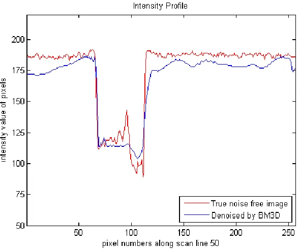
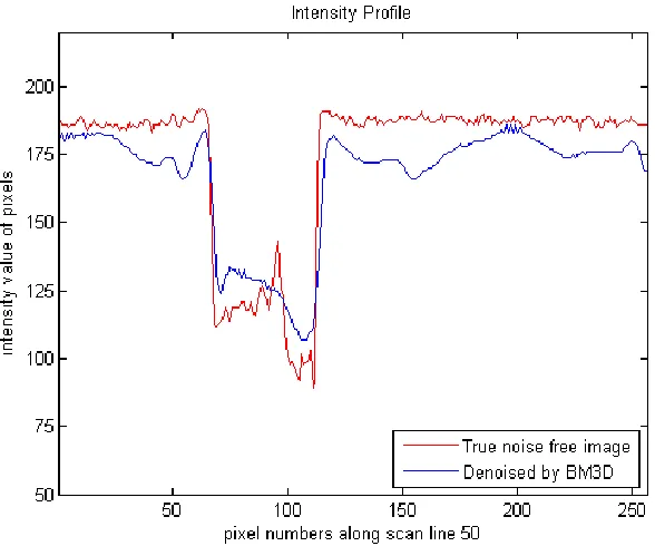
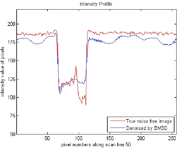
4.2.3 Visual quality comparison and intensity profile ... 48
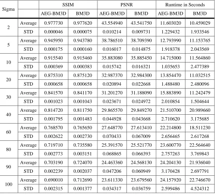
4.2.4 Average SSIM, PSNR, and Runtime Comparison... 64
4.3 Overall results discussion ... 66
Chapter 5 ... 67
vii
5.1 Conclusion ... 67
5.2 Future work ... 68
Bibliography ... 70
Appendices ... 84
Appendix A. PSNR for selected standard images ... 84
Appendix B. SSIM for selected standard images ... 88
Appendix C. Subjective comparison of Boat and Lena ... 92
viii
List of Tables
Table 3-1: Parameters used for different schemes ... 34
Table 3-2: Value of Parameters inherited from BM3D ... 35
Table 3-3: Parameter values for our proposed method ... 37
Table 4-1: PSNR (dB) comparison for Lena image among BM3D, our four experimental
schemes and final proposed method for different noise levels ... 43
Table 4-2: PSNR (dB) comparison for standard Mandril image among BM3D, our four
experimental schemes and final proposed method for different noise levels . 44
Table 4-3: PSNR performance comparison of examined schemes and our proposed
method with BM3D for all 32 images in our test dataset ... 46
Table 4-4: SSIM comparison for standard Lena image among BM3D, our four
experimental schemes and final proposed method for different noise levels . 47
Table 4-5: SSIM comparison for standard Mandril image among BM3D, our four
experimental schemes and final proposed method for different noise levels . 47
Table 4-6: Total SSIM performance comparison of examined schemes and our proposed
method with BM3D for all 32 images in our test dataset ... 48
Table 4-7: Average SSIM, PSNR, and Runtime performance comparison of our proposed
method AEG-BM3D with BM3D for standard Lena image ... 64
Table 4-8: Average SSIM, PSNR, and Runtime performance comparison of our proposed
ix
List of Figures
Figure 2-1: Probability density function for the Gaussian noise model [98]. 7
Figure 2-2: Flowchart of BM3D image denoising algorithm. 16
Figure 3-1: A pictorial demonstration of the major weaknesses of BM3D. (a) Noise free
standard Lena image. (b), (d), and (f) noisy images with different noise
levels. (c), (e), and (g) BM3D denoised image. 22
Figure 3-2: Scheme of data adaptive BM3D with selective median filtering 24
Figure 3-3: Illustration of a window of size (i.e. ) or 2×4+1 (i.e. ) 25
Figure 4-1: Set of less textured noise-free images used for the comparison tests. 39
Figure 4-2: Set of heavily textured noise-free images used for the comparison tests. 40
Figure 4-3: Subjective comparison of denoising performance between BM3D and
AEG-BM3D for standard test image Mandril at noise level . (a) Noise free
Mandril image. (b) Noisy image with . (c) Denoised image using
BM3D, PSNR = 29.1114, SSIM = 0.8495. (d) Denoised image using
AEG-BM3D, PSNR = 29.1224, SSIM = 0.8505. 50
Figure 4-4: Subjective comparison of denoising performance between BM3D and
AEG-BM3D for standard test image Mandril at noise level . (a) Noise free
Mandril image. (b) Noisy image with . (c) Denoised image using
BM3D, PSNR = 26.8046, SSIM = 0.7705. (d) Denoised image using
AEG-BM3D, PSNR = 26.8315, SSIM = 0.7725. 51
Figure 4-5: Subjective comparison of denoising performance between BM3D and
AEG-BM3D for standard test image Mandril at noise level . (a) Noise free
x
BM3D, PSNR = 25.3906, SSIM = 0.6988. (d) Denoised image using
AEG-BM3D, PSNR = 25.3887, SSIM = 0.6989. 52
Figure 4-6: Subjective comparison of denoising performance between BM3D and
AEG-BM3D for standard test image Mandril at noise level . (a) Noise free
Mandril image. (b) Noisy image with . (c) Denoised image using
BM3D, PSNR = 23.3718, SSIM = 0.5680. (d) Denoised image using
AEG-BM3D, PSNR = 23.4056, SSIM = 0.5732. 53
Figure 4-7: Subjective comparison of denoising performance between BM3D and
AEG-BM3D for standard test image Mandril at noise level . (a) Noise free
Mandril image. (b) Noisy image with . (c) Denoised image using
BM3D, PSNR = 21.9692, SSIM = 0.4600. (d) Denoised image using
AEG-BM3D, PSNR = 22.1969, SSIM = 0.4978. 54
Figure 4-8: Subjective comparison of denoising performance between BM3D and
AEG-BM3D for standard test image Mandril at noise level . (a) Noise free
Mandril image. (b) Noisy image with . (c) Denoised image using
BM3D, PSNR = 21.4804, SSIM = 0.4235. (d) Denoised image using
AEG-BM3D, PSNR = 21.8169, SSIM = 0.4634. 55
Figure 4-9: Subjective comparison of denoising performance between BM3D and
AEG-BM3D for standard test image Mandril at noise level . (a) Noise free
Mandril image. (b) Noisy image with . (c) Denoised image using
BM3D, PSNR = 21.0728, SSIM = 0.3991. (d) Denoised image using
AEG-BM3D, PSNR = 21.4881, SSIM = 0.4416. 56
Figure 4-10: Comparison of edge and contrast preservation for zoomed fragment of Boat
image. (a) Noise free fragment. (b)-(e) Noisy fragment with
respectively. (f)-(i) Denoised fragment using BM3D
xi
Figure 4-11: Comparison of edge and contrast preservation for zoomed fragment of Lena
image. (a) Noise free fragment. (b)-(e) Noisy fragment with
respectively. (f)-(i) Denoised fragment using BM3D
(j)-(m) Denoised fragment using AEG-BM3D 58
Figure 4-12: Row number 50 of the standard House image is chosen as the scan line
(presented by a dark red straight line) to generate intensity profiles. 59
Figure 4-13: Intensity profile of House image and denoised image by BM3D at scan Line
50 (σ=80) 61
Figure 4-14: Intensity profile of House image and denoised image by proposed method at
scan line 50 (σ=80) 61
Figure 4-15: Intensity profile of House image and denoised image by BM3D at scan line
50 (σ=90) 62
Figure 4-16: Intensity profile of House image and denoised image by proposed method at
scan line 50 (σ=90) 62
Figure 4-17: Intensity profile of House image and denoised image by BM3D at scan line
50 (σ=100) 63
Figure 4-18: Intensity profile of House image and denoised image by proposed method at
scan line 50 (σ=100) 63
Figure C-1: Subjective comparison of denoising performance between BM3D and
AEG-BM3D for standard test image Boat at noise level . (a) Noise free
Boat image. (b) Noisy image with . (c) Denoised image using BM3D,
PSNR = 30.6902, SSIM = 0.8215. (d) Denoised image using AEG-BM3D,
PSNR = 30.6849, SSIM = 0.8218. 92
Figure C-2: Subjective comparison of denoising performance between BM3D and
AEG-BM3D for standard test image Boat at noise level . (a) Noise free
xii
PSNR = 28.8529, SSIM = 0.7731. (d) Denoised image using AEG-BM3D,
PSNR = 28.8510, SSIM = 0.7736. 93
Figure C-3: Subjective comparison of denoising performance between BM3D and
AEG-BM3D for standard test image Boat at noise level . (a) Noise free
Boat image. (b) Noisy image with . (c) Denoised image using BM3D,
PSNR = 27.3769, SSIM = 0.7256. (d) Denoised image using AEG-BM3D,
PSNR = 27.4322, SSIM = 0.7282. 94
Figure C-4: Subjective comparison of denoising performance between BM3D and
AEG-BM3D for standard test image Boat at noise level . (a) Noise free
Boat image. (b) Noisy image with . (c) Denoised image using BM3D,
PSNR = 25.3550, SSIM = 0.6583. (d) Denoised image using AEG-BM3D,
PSNR = 25.3935, SSIM = 0.6606. 95
Figure C-5: Subjective comparison of denoising performance between BM3D and
AEG-BM3D for standard test image Boat at noise level . (a) Noise free
Boat image. (b) Noisy image with . (c) Denoised image using BM3D,
PSNR = 23.6621, SSIM = 0.6049. (d) Denoised image using AEG-BM3D,
PSNR = 23.9182, SSIM = 0.6006. 96
Figure C-6: Subjective comparison of denoising performance between BM3D and
AEG-BM3D for standard test image Boat at noise level . (a) Noise free
Boat image. (b) Noisy image with . (c) Denoised image using BM3D,
PSNR = 22.8584, SSIM = 0.5771. (d) Denoised image using AEG-BM3D,
PSNR = 23.3414, SSIM = 0.5762. 97
Figure C-7: Subjective comparison of denoising performance between BM3D and
AEG-BM3D for standard test image Boat at noise level . (a) Noise free
Boat image. (b) Noisy image with . (c) Denoised image using
BM3D, PSNR = 22.175, SSIM = 0.5563. (d) Denoised image using
xiii
Figure C-8: Subjective comparison of denoising performance between BM3D and
AEG-BM3D for standard test image Lena at noise level . (a) Noise free
Lena image. (b) Noisy image with . (c) Denoised image using BM3D,
PSNR = 32.9968, SSIM = 0.8749. (d) Denoised image using AEG-BM3D,
PSNR = 33.0008, SSIM = 0.8752. 99
Figure C-9: Subjective comparison of denoising performance between BM3D and
AEG-BM3D for standard test image Lena at noise level . (a) Noise free
Lena image. (b) Noisy image with . (c) Denoised image using BM3D,
PSNR = 31.1574, SSIM = 0.8410. (d) Denoised image using AEG-BM3D,
PSNR = 31.1758, SSIM = 0.8416. 100
Figure C-10: Subjective comparison of denoising performance between BM3D and
AEG-BM3D for standard test image Lena at noise level . (a) Noise free
Lena image. (b) Noisy image with . (c) Denoised image using
BM3D, PSNR = 29.7966, SSIM = 0.8083. (d) Denoised image using
AEG-BM3D, PSNR = 29.8042, SSIM = 0.8117. 101
Figure C-11: Subjective comparison of denoising performance between BM3D and
AEG-BM3D for standard test image Lena at noise level . (a) Noise free
Lena image. (b) Noisy image with . (c) Denoised image using
BM3D, PSNR = 27.7087, SSIM = 0.7699. (d) Denoised image using
AEG-BM3D, PSNR = 27.7289, SSIM = 0.7729. 102
Figure C-12: Subjective comparison of denoising performance between BM3D and
AEG-BM3D for standard test image Lena at noise level . (a) Noise free
Lena image. (b) Noisy image with . (c) Denoised image using
BM3D, PSNR = 25.5006, SSIM = 0.7344. (d) Denoised image using
AEG-BM3D, PSNR = 25.9448, SSIM = 0.7036. 103
Figure C-13: Subjective comparison of denoising performance between BM3D and
AEG-BM3D for standard test image Lena at noise level . (a) Noise free
xiv
BM3D, PSNR = 24.5864, SSIM = 0.7259. (d) Denoised image using
AEG-BM3D, PSNR = 25.3037, SSIM = 0.6933. 104
Figure C-14: Subjective comparison of denoising performance between BM3D and
AEG-BM3D for standard test image Lena at noise level . (a) Noise free
Lena image. (b) Noisy image with . (c) Denoised image using
BM3D, PSNR = 23.7521, SSIM = 0.7134. (d) Denoised image using
1
Chapter 1
1
Introduction
A digital image is composed of set of pixels which is defined as a two dimensional
function, where and are spatial coordinates. The value of at any particular
pair of coordinates is called the gray level or intensity of the image at that location.
The image becomes a digital image when and the values of are all finite, discrete
quantities. These values of are generally referred to as pixels. Pixel values in images
can be noisy. Noise in images is mainly caused by sensors during acquisition,
environments (e.g. poor illumination) or during transmissions. No matter how good the
image acquisition devices are, an image improvement is always sought-after to improve
their range of applications in various fields. The process of estimating the original image
by reducing the noises from noise-contaminated image is referred to as image denoising
in image processing. Image denoising is a very important task in image processing as a
process itself or as an element of other image processing tasks.
Image denoising is a well-studied field and yet it’s still one of the most active research
areas in image processing and computer vision. It’s a pre-requisite for many image
processing tasks such as image segmentation, image restoration, object recognition,
image classification, and image registration, where estimating the true signal is crucial to
accomplish desirable results.
The form of the noise can be additive, which is generally independent of image data, or
2
The formula for additive noise is
1.1
whereas the formula for multiplicative noise is
1.2
Here, represents the location of pixels, is the original signal, while denotes
the noise introduced to form the corrupted image .
Most of the images are assumed to be contaminated by additive random noise and can be
modeled by a Gaussian distribution. Hence, this type of noise is referred to as Additive
White Gaussian Noise (AWGN). AWGN is also probably the simplest and most
commonly used model in the image denoising literature. As AWGN is random in nature
and it corrupts almost all areas of images, it is challenging to remove AWGN from
images. It becomes increasingly difficult to preserve the small details of an image as the
error level increases.
This thesis work proposes a few improvements over state of the art method for reducing
the effect of AWGN, famously known as Block Matching and 3-D Filtering (BM3D) [1].
1.1 Motivations
The BM3D algorithm exploits non-local image modeling through the signature method of
grouping and collaborative filtering in transform domain. It capitalizes on two principal
properties of natural scene images: the existence of mutually similar patches within a
close neighborhood and the local correlation of pixel values within a single patch.
Grouping similar 2D patches into 3D data arrays allows us to exploit both intra-patch
correlation and inter-patch correlation based on the above two assumptions. As a result,
the group enjoys correlation in all three dimensions, allowing a very high sparse
3
linear-transform domain representations which have few high magnitude coefficients and
many low magnitude coefficients. Sparseness refers to the energy compaction property
(i.e. most of the image details are represented by few large coefficients while noise is
spread across a range of small coefficients). This kind of sparse representation allows us
to separate the noise from the true signal by applying shrinkage on the coefficients in
transform domain. Thus BM3D acts as a very efficient and powerful denoiser and to our
knowledge it exhibits the best performance for AWGN.
BM3D exhibits good results when the number of matching blocks in the defined
neighborhood is plenty enough (e.g. repeating patterns, textures and uniformed areas) to
achieve high sparsity, where nonlocal image modeling is suitable. Also the assumption
that image content is highly correlated on a square patch is not always true for natural
image scenes. If the patch contains curved edges, small image details or singularities, the
non-adaptive transform of BM3D cannot produce a sparse representation of the image,
resulting in poorer denoising performance introducing certain artifacts.
The performance of BM3D also sharply degrades as the noise level increases. At
relatively higher noise levels, due to the increase of noisy pixels, it becomes increasingly
harder for BM3D to differentiate between noise and true image textures, edges, and
image details.
1.2 Thesis contributions
To address the problem of BM3D for irregular image shapes or textures, curved edges
and singularities, we propose an Adaptive Edge-Guided Block-Matching and 3D filtering
(AEG-BM3D) algorithm. In our method, we try to adapt the estimation of pixel values
according the edge activity found in a given block. We extract the edges from the
corrupted image after the first stage of BM3D and use this as guidance to better estimate
the pixel values. The edge information allows us to choose different block sizes for
different types of regions within the same image. Our method tries to integrate the local
4
To address the performance issue of BM3D for higher noise levels, we also proposed a
simple denoising pre-filter to show that the pre-filters can effectively increase the
performance of the denoising at little computational overhead when the additive noise is
strong in images. We applied a simple selective median filter based on an empirically
selected threshold value on the raw corrupted input image. That is, we don’t apply the
median filter for all the image pixels, except the one which has been classified as a
corrupted one. Our method searches the whole image for corrupted pixels in a raster scan
fashion, and we apply the filter only for the pixels which is highly likely to be corrupted.
Experimental results show that the proposed method shows a significant improvement
over current state of the art BM3D algorithm in terms of both subjective and objective
evaluation, particularly when the noise level is high ( ).
1.3 Thesis outline
This thesis is divided into five chapters including this introductory discussion, Chapter 1.
The rest of the thesis is organized as follows. Chapter 2 discusses the noise model
considered for our work. It also presents a brief introduction of the vast field of image
denoising, roughly classified into spatial domain filters and transform domain filters. At
the end of this chapter we discussed our method of interest that is, Block Matching and
3D Filtering or BM3D, and its various variants proposed by various literatures till now,
along with its applications in practical image processing problems. In Chapter 3, we
described our proposed method in detail. Experimental results and relevant analysis are
presented in Chapter 4. Finally, Chapter 5 offers the concluding remarks and future
5
Chapter 2
2
Background
Noise models are of particular importance in image denoising as most denoising methods
work well with a particular noise model. Probabilistic models best reflect the randomness
of the noise within images. In image denoising applications, parametric models (with few
parameters) of the probability density function (PDF) are most commonly used. This
chapter introduces the noise model considered for this thesis, AWGN, along with a
detailed review of existing filters to remove this type noise.
2.1 Additive white Gaussian noise
A random signal with flat (constant) power spectral density is known as white noise. In
Additive White Gaussian Noise the image is contaminated with a linear combination of
white noise with a constant spectral density, where the amplitude has a Gaussian
distribution. Most often, it is assumed that Gaussian noise necessarily means white noise,
which is not correct also. The term Gaussian refers to the probability density function,
that is, the probability distribution with respect to the signal value, while the term white
refers to the way signal power is distributed over time among frequencies. It is possible to
have Poisson white noise, for example, just like Gaussian white noise.
Gaussian noise is the most common type of noise found in natural images. It represents
many real world situations and generates mathematically tractable model in both the
spatial and transform domain. White Gaussian noise is also commonly found in other
fields than image processing such as music, electronics engineering, and acoustics etc.
6
stage and the transmission stage. During acquisition, noise may be generated by sensor
due to poor illumination and/or high temperature while electronic circuit may generate
noise during transmission.
Moreover, dealing with the uniform Gaussian noise makes the discussion of image
denoising methods much easier. Two papers published in 2011 on the Anscombe
variance-stabilizing transform by M. Mäkitalo and A. Foi (for low-count Poisson noise)
[39] and A. Foi (for Rician noise) [40] argue that, when combined with suitable forward
and inverse variance stabilizing transformation (VST) transformations, methods
designed for AWGN work just as well as ad hoc algorithms based on signal dependent
noise models. This also explains why, in most of the image denoising literature noise is
assumed to uniform, white, and Gaussian.
The PDF of a Gaussian random variable, ω,is given by
2.1
The mean of ω is zero and its variance is 1.
A general Gaussian random variable is given by
2.2
where, the mean of the variable z is µ, whereas is the variance of z.
We can rewrite the probability density function of Equation 2.1 as follows:
2.3
7
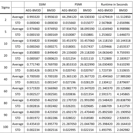
Figure 2-1: Probability density function for the Gaussian noise model [98].
Figure 2-1 illustrates the Gaussian probability density function. Approximately 68.27%
of the values are contained between and 95.45% of the values are contained
between .
2.2 Existing filters to remove AWGN
In this section we will try to give an introduction to the common AWGN filtering
techniques in past few decades. Throughout the rest of this thesis, unless the noise model
is explicitly specified, we implicitly assume the AWGN model. We broadly classify the
image denoising filters into two major categories: Spatial Domain Filters and Transform
Domain Filters. We will also attempt to group them together according to their
8
2.2.1
Spatial Domain Filters
One of the most common ways to reduce noise from images is to use Range filters. These
classes of filters are computationally simple to calculate, easy to implement and are
neighborhoods adaptive to the image data. Bilateral filter [41], the SUSAN filter [93] and
the sigma filter [43] are noteworthy among these filters. The range filters use nonlinear
weighted averaging with adaptive weights that depends on the spatial distance and the
photometric distance, which is the distance between the pixel intensities (i.e. the image
range). The general equation for the range filters is
2.4
where z(k) is the noisy signal and y(x) is the filtered or denoised signal. The function gsp
depends on the spatial distance between pixels and the function grng depends on the
distance between intensities. The grng function here gives the range filters ability to adapt
to image data and better preserve salient details such as edges, without blurring while
doing spatial smoothing in regions with relatively homogeneous intensities. However, as
the noise level increases it becomes increasingly difficult to differentiate between noisy
pixels and their noise free counterparts with edges, resulting in decreased performance of
range filters. Staircase effects are also visible in these types of filters. One approach to
overcome this drawback is to take advantage of the similarities between image
neighborhoods (e.g. nonlocal filters), which will be discussed later in this section.
Some satisfactory results have been obtained for image restoration through Bayesian
filters. The general idea in the Bayesian estimation framework is to find the noise free
image given the prior information of the noise and the observed noisy image z. The
Bayes formula for the posterior probability is given below:
9
Here, z is the image being observed or the noisy image, while γ is an estimation of the
noise free image y, the image prior pprior(γ) denotes the probability that γ belongs to
family of noise free images, the likelihood (or data fit) pfit(z| γ) is the conditional
probability of generating z according to the assumed noise model from γ, and pz(z) is the
marginal probability of obtaining the noisy realization z. Bayesian estimation based filters
are based on finding a solution γ using the posterior probability ppost(γ|z) from Equation
2.5. The main challenge for Bayesian estimation in image processing is the derivation of
a better image prior pprior [89].
Another class of spatial domain filters is the Variational and PDE-based filters. The
Total Variation (TV) minimization was introduced by Rudin, Osher and Fatemi [44] as a
regularizing functional for image denoising. Total variation denoising (TVD) is defined
in terms of an optimization problem by minimizing a particular cost function. TVD
removes unwanted detail whilst preserving sharp edges in the original signal. Numerous
methods have been proposed to solve the TDV problem [45] [46] [47]. The original TV
model considered the removed noise as an error and no longer considered them in the
reconstruction process. However, some structures and textures are always present in the
removed errors. Later on, the authors tried to reduce this effect by using the Rudin,
Osher, and Fatemi total variation minimization iteratively [48] [49]. Total variation is
also used by researchers for general image restoration problems such as compressed
sensing, interpolation, deconvolution, etc. [50] [51].
Partial differential equations (PDE) based diffusion techniques are yet another effective
way to denoise images and are very similar to variational techniques. These technique has
wide range of application in image processing [53] [54] such as image
enhancement/denoising, edge detection, and flow field visualization, since the first model
was introduced by Perona and Malik in 1987 [52]. This type of diffusion can effectively
remove noises and at the same time can enhance edges. One of the most widely used
PDE formulation in image processing is the anisotropic diffusion proposed my Perona
and Malik in 1990 [55], which preserves the edges by guiding the smoothing with spatial
derivative. A range of applications of PDEs in image processing can be found [53] [54]
10
In recent years, the Non-Local means (NL-means) algorithm, has attained great deal of
attention within the image processing community [57] [58]. A detailed study of
NL-means with various extensions can be found in [58]. Fundamentally, it is a relatively
simple generalization of the range filters like bilateral filter, in particular the point-wise
photometric term in the similarity kernel of range filters is replaced by the block-based
(or patch-based) similarity kernel. Another difference is that the geometric distance
between the blocks is in fact ignored, which leads to the strong contribution of blocks that
may not be essentially near the pixel of interest. The NL-means algorithm tries to exploit
the property that natural images have high degree of self-similarity or redundancy
between image neighborhoods, from which the name Non-Local originated. It is worth
mentioning that the NL-means filters exploits resemblance between surrounding
neighborhoods while the range filters exploits resemblance between individual pixels.
Boulanger and Kervrann [59] demonstrated the true potential of NL-means filters with
the optimal spatial adaptation (OSA) which is based on adaptive estimation
neighborhoods. In recent years, the non-local priors variational formulation has also
became a very popular research topic [60] [61] [62] in the image processing community.
In these approaches, the authors have formulated the nonlocal image modeling as
particular regularization functionals.
2.2.2
Transform Domain Filters
Since their introduction, multiscale transforms such as wavelets, ridgelets, curvelets etc.
[64] [65] [66] [67]. has been widely use by the image processing community to get sparse
representation of images [68]. A recent study [63] showed that natural images contain
areas which are similar to other areas at the same resolution/orientation and across
resolution/orientations. Multiscale transform is concerned with representation and
analysis of signal at more than one resolution based on the fact that features that might go
undetected at one resolution may be easily detected at another resolution. One of the most
commonly used multiscale transform is wavelet decomposition. In wavelet
decomposition, a wavelet generating function ψ of zero mean is used to generate a
11
2.6
where, s and u are the scale and shift (translation) parameters respectively. Multiscale
decompositions are localized in both time and frequency and, possibly with varying
orientation whereas transforms with fixed spatial localization (e.g. short time Fourier
transform) or trigonometric transforms (e.g. DCT, DFT) are only localized in frequency.
In recent years, the over-completeness of multiscale representations has led to much
interesting research problems in image restoration [68] [69] [70]. Formally, an
over-complete dictionary contains prototype signal-atoms and any signal can be represented by
more than one combination of these atoms. Over-completeness is required for translation
invariance [69] of multiscale representations. Dual-tree complex wavelet [71] and
steerable pyramid [72] [73] are amongst the most commonly used over-complete
transforms.
All of the above mentioned methods use fixed dictionaries. Dictionaries can also be
adaptive to the input image. Independent Component Analysis (ICA) [75] and Principal
Component Analysis (PCA) [74] are two well recognized such data adaptive transforms
that have found lots of interesting applications in image processing. PCA is particularly
successful in reconstructing oscillatory patterns and textures while ICA has been
successfully applied in image denoising, as it can achieve better sparsity for natural
images. To name a few other adaptive transform domain filters that have been applied in
image denoising very successfully, we would like to mention shape adaptive DCT or
SA-DCT [86], point-wise shape adaptive DCT (P.SA-DCT) [76] [87], and K-SVD [34].
Among these methods we would like single out the state of the art method, K-SVD, a
generalization of the k-means clustering method, which is regarded as one of the major
advancements in the field of adaptive transform domain filters. It is an iterative method
that iteratively alternates between sparse coding coefficients of the examples based on the
current dictionary and a method of updating the atoms in the dictionary to better fit the
12
Among the shrinkage filters, Wiener filters showed good potential for denoising. For
AWGN a parametric version of Weiner filter, , is used which is defined by the
following equation,
2.7
where, is the complex conjugate of the degradation function and is a
pre specified constant. However, wiener filtering for white noise tends to weaken the
energy signal spectral coefficients leading to poor denoising performance.
In recent years, wavelet shrinkage filters has became one of the most important and
powerful tools for image and video processing. The wavelet transform has the important
properties such as compression or sparsity, which means that wavelet transforms tends to
be sparse. Therefore, wavelet shrinkage is based on the fact that in the wavelet domain, a
signal is represented with few large coefficients, which are processed or kept according to
particular shrinkage function, whereas noises in signal is distributed across small
coefficients, which are removed. The WaveShrink or the shrinkage of wavelet
coefficients was introduced and extensively studied by Donoho and Johnstone in their
seminal work [77] [78]. Donoho and Johnstone proposed two basic shrinkage algorithms
[77]: soft thresholding and hard-thresholding, governed by the following equations:
2.8
and
. 2.9
Here, τ is the thresholding parameter, which is predefined, and selection of an optimal
value for τ is a critical problem. The authors recognized this issue and proposed an
expression of the optimal threshold as a function of the noise variance σ2 and the number
13
2.10
This is known as universal threshold, application of which in wavelet domain is called
VisuShrink [77].
The above mentioned shrinkages are non-adaptive and don’t perform satisfactorily in
most cases. A lot of work has been done to propose different data-adaptive thresholding
methods to improve the performance of the WaveShrink estimators. Donoho and
Johnstone themselves acknowledged this drawback and proposed the SureShrink
approach [78] in which they introduced an data adaptive threshold that chooses the
thresholding parameter, , by minimizing the Steins unbiased risk estimator (SURE) [79].
More recent studies have shown that better denoising can be achieved by exploiting
intra-scale and inter-intra-scale correlations of the wavelet coefficients. One such method is
ProbShrink [80], which is driven by the estimation of the probability that a given
coefficient contains considerable level of information. The bivariate shrinkage or
BiShrink [81] exploits inter-scale correlations by using a new non-gaussian bivariate
distribution to model the dependencies. In another article [82], the authors, Sendur and
Selesnick, accounted the intra-scale dependency by extending their previous approach.
Luisier et al. proposed a new SURE-based method SURE-LET [83] to wavelet based
image denoising exploiting inter-scale correlation, which was later extended by Yan et al.
[84] including inter-scale correlation. More recently, the trivariate shrinkage was
introduced by Yu et al. [85], here wavelet coefficients are modeled as a trivariate
Gaussian distribution and then a trivariate shrinkage filter by using the maximum a
posteriori (MAP) estimator is then derived. It successfully models both the inter-scale
and intra-scale correlations of wavelet coefficients. All these shrinkage based methods
discussed above rely on one fundamental property, the sparsity of natural images in
wavelet domain.
However for our study, the most important class of filters is the non-local transform
domain filters. This class of filters is blessed by both the sparsity of the transform domain
14
transform, which is a multi-scale adaptive transform in which the main component is a
modified Haar dyadic decomposition. Though this method doesn’t exhibit competitive
results in terms of MSE, it effectively reconstructs image details. BM3D, our algorithm
of interest, falls in this class of non-local transform domain filters, which is a recent
development by Dabov et al. [1]. BM3D is basically a generalization of their previous
work [2]. In that work, the authors exploited nonlocal modeling by grouping similar
neighboring blocks, sparsity in transform domain by collaborative filtering and
aggregation by combining different estimates from the previous collaborative filtering
stage. Based on the achievement of BM3D in image denoising it is extended to other
image processing tasks successfully (e.g. image restoration, deblurring, sharpening and
video denoising). A detailed discussion on BM3D is in order.
2.3 Introduction to BM3D and its Variants
In past few years there has been a growing interest in the development of sparse
representation of signals. In image denoising, this approach has gained much traction and
led to several state of the art denoising algorithms, such as K-SVD [34] and BM3D [1].
Image denoising by sparse 3D transform-domain collaborative filtering [1], famously
known as block-matching and 3D filtering, which exploits nonlocal image modeling [5]
with a method termed grouping and collaborative filtering was proposed in 2007 by
Dabov et al. It was an improvement over the novel algorithm [2] proposed by the same
authors. In this section we will investigate the different aspects of the BM3D algorithm
giving a sufficient introduction to the background of BM3D, to understand the basic
underpinnings of the method. We also try to provide a comprehensive analysis of BM3D
and its variants on various natural images, as well as describing the limitations of existing
methods.
BM3D is currently known as the state of the art method for image denoising and
outperforms all other algorithm when it comes to removing AWGN at a reasonable
computational complexity. BM3D relies on the assumption that an image has a locally
15
grouping similar 2D fragments into 3D data array which the authors called “groups”.
Because each block in the group was chosen according to some similarity measure with
respect to a reference block, the use of a higher dimensional filtering of each group was
possible. This exploits the potential similarity (correlation, affinity, etc.) between grouped
blocks to estimate the true signal in each of them by producing a highly sparse
representation in 3D transform domain, so that the noise can be removed by wavelet
shrinkage. This approach of exploiting similarity and estimating the original signal is
called as collaborative filtering. Collaborative filtering has three successive steps:
1. For each reference patch, find similar patches from the input image by classifying
them according to some similarity criteria and transform them into a 3D data
array by grouping the matched 2D blocks.
2. Shrinkage of the coefficients in transformed 3D spectrum is applied to attenuate
the noise.
3. Apply inverse 3D transform to the shrunken coefficients and return the obtained
2D estimates of the grouped blocks to their original positions.
In this way the collaborative filtering process gives a 3D estimation of the jointly filtered
2D blocks. As the grouped 2D blocks are similar, the transformation can achieve a very
high sparse representation of the original signal. This process reveals the finest details
shared by grouped blocks by preserving the unique features of each individual block.
2.3.1
Architecture of the BM3D algorithm
The BM3D algorithm can be distinctively decomposed into two almost identical steps
16
The general concept of the two steps in BM3D is as follows:
Step 1: In this step an intermediate (i.e. basic estimate) denoised image is estimated using
hard thresholding during the collaborative filtering process by taking the original image
(noisy image) as the input:
a) Grouping and collaborative filtering: The input image is processed block by
block. These blocks are called reference blocks. For each reference block similar
blocks to the currently processed one are found using a similarity measure (block
matching). A 3D group (array) is then built by stacking the matched blocks and a
collaborative filter is applied to the grouped blocks. In this step, hard thresholding
is applied during shrinkage of the coefficients in the transform domain.
b) Aggregation: After collaborative filtering, we get an estimate of each block and a
variable number of estimates for each pixel due to the overlapping of blocks. The
output of the first step is obtained by weighted averaging of all the achieved
block-wise estimates that have overlapped.
Step 2: This step produces the final denoised estimate based on both the input noisy
image and the basic estimate obtained from step 1. Here, instead of hard thresholding,
R 3D transform Hard thresholding Inverse 3D transform Block-wise estimate Aggregation Grouping by block-matching Step 1 R 3D transform Wiener filtering Inverse 3D transform Block-wise estimate Aggregation Final Wiener estimate Grouping by block-matching Step 2 noisy image Weight Weight
17
Wiener filtering [35] is used as the shrinkage method. It applies Wiener filtering to the
original noisy input image by using the basic estimate obtained from step 1 as an oracle:
a) Grouping and collaborative filtering: The basic estimate is used to find locations
of the matched blocks similar to the currently processed one. Two 3D groups
(arrays) are formed from the locations of the basic estimate, one from the original
input (noisy) image and the other from the basic estimate. Then, collaborative
filtering is applied on the noisy image. Here, a 3D transform is applied on both
groups and during shrinkage, Wiener filtering is applied on the noisy image using
the energy spectrum of the basic image as the true energy spectrum.
b) Aggregation: By aggregating all the estimates using a weighted average the final
denoised image is obtained.
2.3.2
Applications of BM3D
Though the major application of BM3D is image denoising, it is shown to be equally
effective by Dabov et al. [11][12] in different areas of image processing such as generic
image and video restoration, image deblurring [7][8], image sharpening [9][10] and video
denoising [13][14][15]. In this section we address different applications of BM3D, its
limitations, and published extensions.
2.3.2.1
BM3D in medical imaging
BM3D approach is used to reconstruct medical imagery. Significant denoising
performance in clinical MRI image denoising has been attained by optimizing the cost
functions for noise removal [16]. ART-BM3D [17] is applied to limited-angle
reconstruction in CT reconstruction which uses BM3D to find a sparse representation of
the original image. Kang et al. [18] applied adaptive BM3D by estimating the noise using
a wavelet based noise estimation technique [19] for low-radiation dose coronary CT
angiography images. Other similar efforts [20][21][22][23][24][25] of medical image
18
2.3.2.2
Application in removing other kinds of noise than AWGN
BM3D is also proven to be effective for removing other kinds of noise than AWGN. In
the PIDD-BM3D algorithm Danielyan et al. [26] used data adaptive BM3D-frames and
formulated image reconstruction as a generalized Nash equilibrium problem to remove
Poisson noise from images. Begovic et al. [27] proposed two separate contrast
enhancement and denoising framework based on two popular techniques, K-SVD and
BM3D for solar images corrupted with a mixture of pixel-dependent Poisson noise and
white Gaussian noise. BM3D is also successfully tailored to remove power-law noise
[28] and correlated noise from images [29].
2.3.3
Limitations and enhancements of BM3D
BM3D has generated much interest in the field of image and video denoising since it was
published in 2007, followed by several improvements proposed by Dabov et al., quickly
followed by different variations, enhancements and applications of BM3D by the image
processing community. Dabov et al. [3] exploited both locally adaptive anisotropic
estimation and non-local image modeling, which only improves the denoising
performance when the noise level is low but for higher noise level its performance is
inferior to BM3D [1]. Dabov et al. also exploited local shape-adaptive anisotropic
estimation, principal component analysis (PCA) and nonlocal image modeling [4] which
preserves image details and introduces few artifacts than [1], but only shown to be
effective up to noise level of standard deviation 35.
BM3D performs best when the number of matched blocks is higher (e.g., textures,
regular shaped image structures, or uniform areas). It is not effective when a large
amount of matching blocks is not found. As the content of natural images is not always
highly correlated and large numbers of matching blocks are not always guaranteed in
natural images, BM3D introduces artifacts and doesn’t perform as well. Also, if the
19
noise itself. In these situations, though it preserves the fine image details after denoising,
it can blur the edges after the collaborative filtering and aggregation step. In the
transform domain the edges and the noises are not distinguishable and this forces the
filtering process to remove some of the edge information making edges blurry. Several
enhancements were proposed to overcome these shortcomings of BM3D [1]. The
shortcomings of BM3D and efforts made to mitigate these issues are described below.
2.3.3.1
Performance decreases if the noise level is high and
artifact appears:
Though BM3D introduces fewer artifacts than other denoising methods it still exhibits a
few artifacts under certain conditions. A number of periodic artifacts appears when
2D-Bior1.5 (bi-orthogonal spline wavelet with vanishing moments of the decomposing and
the reconstructing wavelet functions of 1 and 5, respectively) is replaced by 2D-DCT for
high noise level ( ) and the block size ( ) is increased to 12 from 8 in the first
step of BM3D [1]. Hou et al. argued [36] that these changes are unnecessary and
proposed a scheme which gives better peak signal to noise ratio (PSNR) and also
superior subjective visual quality than [1]. The authors simply changed the DCT
transform to Bior1.5, increasing the maximum number of matched blocks ( ) by
increasing the maximum threshold ( ) while matching. Hou et al. [32] separated the
3D transform of BM3D to two steps 1D transform, which also shows better denoising
performance than original BM3D algorithm for greater noise levels in terms of peak
signal-to-noise ratio, structural similarity and subjective visual quality, and introduces
lesser periodic artifacts. BM3D is more effective when it finds a sufficient number of
matches for the reference patch. Separating edges from noise becomes increasingly
difficult as the level of noise increases which results in poor matching. The calculation of
each pixel values by weighted averaging of block-wise estimates also leads to blurring of
edges as averaging works like a low pass filter. These issues are addressed by Chen and
Wu [6] and they proposed a bounded BM3D approach which partitions the image in
several regions before block matching. In addition, the authors used partial block
matching instead of the block as a whole if the block contains edges and it belongs to
20
performance, when the noise standard deviation reaches 40, is proposed by Li et al. [33],
they combine BM3D with Tetrolet prefiltering [92]. Here the Tetrolet transform is
applied to the initial noisy image to remove part of the noise before executing BM3D.
Though this approach shows slightly lower denoising performance than BM3D-SAPCA
[4], its execution time is significantly less than the later one.
2.3.3.2
The values of the parameters in BM3D are fixed for all
images:
The values of all the parameters are given a priori, irrespective of the type of image and
the level of noise provided as input. This feature of BM3D sometimes can lead to poor
denoising performance. One important such parameter is the threshold value in the
shrinkage step. Zhang et al. [30] used an adaptive approach that applies a weak (i.e. low)
threshold for low activity (flat) blocks and a strong (i.e. high) threshold for high activity
(detailed) blocks based on Structural SIMilarity (SSIM) between similar blocks. The
authors claimed that this method gives comparable performance for low noise levels but
shows better denoising performance for high noise levels. BM3D relies on the sparsity of
the image in the transform domain. Sparsity of the blocks is not achievable when the
image contains fine details, curved edges or singularities. Sparsity is also hard to achieve
when the level of noise is elevated. To overcome this difficulty, Poderico et al. [31]
proposed a modified BM3D approach that works on the shrinkage parameter when
enough sparsity is not achievable. They proposed a more agile and smoother shrinkage
based on Smooth Sigmoid-Based Shrinkage, resulting in better denoising performance
especially for large noise levels [37]. Mittal et al. [38] showed that a blind parameter
estimation for BM3D based on natural scene statistics, which maps statistical features to
noise variance using support vector machine regressor exhibits better denoising
performance than the reference BM3D implementation in [1], measured using the
21
Chapter 3
3
Methodology
BM3D is one of the most powerful and efficient image denoising algorithms available
currently. In recent years, it has gain much interest within the image processing
community due to its improved performance, both in terms of reducing noise from
images and in terms of maintaining visual image details. It takes advantage of a locally
sparse representation of images in the transform domain. In BM3D, highly sparse
representation of images in the transform domain is achieved through grouping and
collaborative filtering followed by a weighted averaging. Enhancement of sparsity is
achieved by finding and grouping similar 2D image blocks and stacking them together
into 3D arrays or groups. The data exhibits a high level of correlation due to inherent
similarity in a group. Besides reducing the noise, the collaborative filtering procedure
reveals even the finest image details shared by grouped blocks, while preserving the
unique features of each block.
Despite excellent results, BM3D has certain drawbacks and some improvement is still
possible, especially for higher noise levels. BM3D produces many artifacts when the
noise level is high ( ). The performance of noise reduction also significantly drops
as the noise level increases. When the noise level is large, block matching is not reliable
any more, as blocks which are not similar to the referenced block can easily be grouped
together into the 3D array, resulting in less sparser representation in transform domain. It
also tends to give poor visual results when exposed to micro-textured zones in natural
images. Another important drawback of BM3D is that it blurs sharp edges, as it uses a
weighted averaging at the end of each step (i.e. first step and second step), which works
22
be observed in almost all of its denoised images. The Lena image in Figure 3-1, for
example, demonstrates all these shortcoming of BM3D for higher noise levels:
(a) noise free image
(b) noisy image ( ) (c) denoised by BM3D
(d) noisy image ( ) (e) denoised by BM3D
(f) noisy image ( ) (g) denoised by BM3D
23
In this thesis, we present an enhancement over BM3D to overcome its above mentioned
limitations. For higher noise levels some noisy pixel can be detected and restored based
on its neighboring pixels to reduce the effect of higher noise during grouping and
collaborative filtering. We used this pre-filter when the noise level is high enough
. Also to reduce the effect of blurring sharp edges, we used an edge guided pixel
estimation technique. Experimental results show that our method outperforms BM3D in
terms of both objective and subjective measures. The proposed method also better
preserves contrast and edges as compared to BM3D, in particular for higher noise levels.
3.1 Data adaptive BM3D with selective median filtering
Our proposed method is divided into three major steps which are illustrated in Figure 3-2.
In the first step we detect the noisy pixels and try to restore these values using median
filter. This pre-filtering is applied only for higher noise levels . If the noise level
is low or if a pixel cannot be decided as corrupted, this first step works as an
identity filter. Here we assume standard deviation of noise is a priori knowledge, as it can
be accurately estimated [99]. Moreover, assessing the value of sigma is out of the scope
of my thesis. In second step, we group the matching blocks into a 3D data array for each
reference block and apply collaborative hard thresholding for two different block sizes
based on the noise level present in the input noisy image as described in Section 3.3.
Unlike BM3D, here we get two preliminary basic estimates which we process to produce
the final estimate. We always choose the basic estimate with block size for
determining the edge map. After that, based on the obtained edge map, we aggregate the
estimation from the two different preliminary basic estimates, producing the final basic
estimate. Then together with the pre-filtered noisy image we fed this more refined basic
estimate as an oracle into the collaborative Wiener filtering stage which is identical to the
24
R
3D transform Hard thresholding Inverse 3D transform Block-wise estimate Aggregation Intermediate basic estiamtes Edge detector Edge map Data Adaptive Aggregation Basic estimate Grouping by block-matching Noisy Image Noisy pixel Detection Pixel restoration Pre-filtered image Step 1 Step 2R
3D transform Wiener filtering Inverse 3D transform Block-wise estimate Aggregation Final Wiener estimate Grouping by block-matching Step 3 Threshold ThresholdFigure 3-2: Scheme of data adaptive BM3D with selective median filtering
Let us assume an image has been corrupted by AWGN resulting in a noisy image of the form.
3.1
where y is the uncorrupted or noiseless image, x represents the pixels of an image in 2D
spatial domain , η is independent and identically distributed zero mean AWGN
25
3.1.1
First step: Selective pixel restoration with median filter
In this step we apply a simple decision-based linear filter to reduce noisy pixels from the
image before applying the actual denoising method. This approach gives considerably
good results for higher noise levels.
Figure 3-3: Illustration of a window of size (i.e. ) or (i.e. )
We use a sliding window method from left to right, top to bottom for each pixel location
to identify the noisy pixel and then restore it subsequently. For this section, with we
denote a filter window of size or taken from the noisy input image z,
, 3.2
where or is the center pixel of the window under processing. For our work, we
use a filter window (depicted in Figure 3-3) centered at x,
. 3.3
To identify the noisy pixel we use a binary classification method to classify the pixel in
consideration as corrupted or not corrupted, based on the current pixel value and its
neighboring pixel values. The current pixel can be classified as corrupted if it is
significantly lower or greater than all other pixel values in the considered neighborhood.
If the current pixel is a maximum or a minimum, we sort the pixel values (excluding )
26
The re-arranged vector is shown below
, 3.4
where are the pixel values of the window sorted in ascending
order. To classify the current pixel, we choose a simple classifier that operates on the
differences of the current input pixel and maximum or minimum of the vector, :
, 3.5
where is a threshold value determined through empirical analysis. If the pixel is
classified as corrupted (i.e. ) then we use a median filtering function on the
window to determine the value of the pixel and replace it. Otherwise, the original
pixel value is kept,
, 3.6
where SMEDIAN refers to the selective median operation. The effect of this simple
selective prefilter is considerable for noisy images with relatively higher noise levels,
where the contrast and edges are best preserved with a higher peak signal-to-noise ratio
(PSNR) in denoised images than the original BM3D algorithm [1].
3.1.2
Second step: data adaptive estimation of the basic denoised
image
In this step we obtain the basic estimate using the pre-filtered version of the noisy image.
We follow the following procedure for two different block sizes of , and , depending on the noise level present in the examined image. Unless otherwise mentioned,
for the rest of this step we will drop the subscript guide and est as the process is similar
for both the case.
Let us denote the basic estimate by and the final estimate by . We define Zx
27
Zx is the coordinate of the top left corner of the patch. In other word, we can say that the
patch Zx is located at location in the image . A 3D group or a group of selected 2D
patches is denoted by a bold face capital letter with a subscript representing the set of its
grouped patches coordinates (e.g. Zs represents a collection of 2D patches composed of
patches Zx located at ). As we have two near identical steps in BM3D we use
the superscript ht (stands for hard thresholding) and wie (stands for Wiener filtering) to
represent the parameters in the first step and the second step respectively. That is, the
patch size used in first step is denoted by and the patch size used in second step is
denoted by . We process the blocks in sliding-window manner by following a raster
scan where each next block is taken with a fixed pixel shift from the previous one. This
ensures there is at least one estimate for each image pixel. We denote the currently
processed block by and call it reference block.
Firstly, we find the blocks that are similar to the reference one within a fixed
neighborhood. We define the similarity based on the block-distance and only consider
those blocks whose distance is less than a pre-defined threshold. The distance is obtained
by applying a normalized 2D linear transform on both blocks followed by a
hard-thresholding on the obtained coefficients.
’
3.7
here, is the distance between the two blocks in consideration. ϒʹ denotes the
hard thresholding operator with threshold value and denotes the linear
transform.
By applying the above equation and defining a maximum distance to match the
similar blocks we get the coordinates of a set of blocks, , that are similar to ,
![Figure 2-1: Probability density function for the Gaussian noise model [98].](https://thumb-us.123doks.com/thumbv2/123dok_us/7774196.1281335/22.612.208.447.80.304/figure-probability-density-function-for-gaussian-noise-model.webp)