Robust Sparse Component Analysis Based on a Generalized Hough Transform

Volume 2007, Article ID 52105,13pages doi:10.1155/2007/52105

Research Article

Robust Sparse Component Analysis Based on

a Generalized Hough Transform

Fabian J. Theis,1_{Pando Georgiev,}2_{and Andrzej Cichocki}3, 4

1_{Institute of Biophysics, University of Regensburg, 93040 Regensburg, Germany}

2_{ECECS Department and Department of Mathematical Sciences, University of Cincinnati, Cincinnati, OH 45221, USA} 3_{BSI RIKEN, Laboratory for Advanced Brain Signal Processing, 2-1, Hirosawa, Wako, Saitama 351-0198, Japan} 4_{Faculty of Electrical Engineering, Warsaw University of Technology, Pl. Politechniki 1, 00-661 Warsaw, Poland}

Received 21 October 2005; Revised 11 April 2006; Accepted 11 June 2006

Recommended by Frank Ehlers

An algorithm called Hough SCA is presented for recovering the matrixAinx(t)=As(t), wherex(t) is a multivariate observed signal, possibly is of lower dimension than the unknown sourcess(t). They are assumed to be sparse in the sense that at every time instantt,s(t) has fewer nonzero elements than the dimension ofx(t). The presented algorithm performs a global search for hyperplane clusters within the mixture space by gathering possible hyperplane parameters within a Hough accumulator tensor. This renders the algorithm immune to the many local minima typically exhibited by the corresponding cost function. In contrast to previous approaches, Hough SCA is linear in the sample number and independent of the source dimension as well as robust against noise and outliers. Experiments demonstrate the flexibility of the proposed algorithm.

Copyright © 2007 Fabian J. Theis et al. This is an open access article distributed under the Creative Commons Attribution License, which permits unrestricted use, distribution, and reproduction in any medium, provided the original work is properly cited.

1. INTRODUCTION

One goal of multichannel signal analysis lies in the detec-tion of underlying sources within some given set of obser-vations. If both the mixture process and the sources are un-known, this is denoted asblind source separation(BSS). BSS can be applied in many different fields such as medical and biological data analysis, broadcasting systems, and audio and image processing. In order to decompose the data set, dif-ferent assumptions on the sources have to be made. The most common assumption currently used is statistical in-dependence of the sources, which leads to the task of inde-pendent component analysis (ICA); see, for instance, [1, 2] and references therein. ICA very successfully separates data in the linear complete case, when as many signals as un-derlying sources are observed, and in this case the mixing matrix and the sources are identifiable except for permu-tation and scaling [3, 4]. In the overcomplete or underde-termined case, fewer observations than sources are given. It can be shown that the mixing matrix can still be recov-ered [5], but source identifiability does not hold. In or-der to approximately detect the sources, additional require-ments have to be made, usually sparsity of the sources [6–

8].

Recently, we have introduced a novel measure for spar-sity and shown [9] that based on sparsity alone, we can still detect both mixing matrix and sources uniquely except for trivial indeterminacies (sparse component analysis (SCA)). In that paper, we have also proposed an algorithm based on ran-dom sampling for reconstructing the mixing matrix and the sources, but the focus of the paper was on the model, and the matrix estimation algorithm turned out to be not very ro-bust against noise and outliers, and could therefore not eas-ily be applied in high dimensions due to the involved com-binatorial searches. In the present manuscript, a new algo-rithm is proposed for SCA, that is, for decomposing a data setx(1),. . .,x(T) ∈ Rm _{modeled by an (m×T)-matrixX} linearly intoX=AS, where then-dimensional sourcesS =

The Hough transform [10] is a standard tool in image analysis that allows recognition of global patterns in an image space by recognizing local patterns, ideally a point, in a trans-formed parameter space. It is particularly useful when the patterns in question are sparsely digitized, contain “holes,” or have been taking in noisy environments. The basic idea of this technique is to map parameterized objects such as straight lines, polynomials, or circles to a suitable parame-ter space. The main application of the Hough transform lies in the field of image processing in order to find straight lines, centers of circles with a fixed radius, parabolas, and so forth in images.

The Hough transform has been used in a somewhat ad hoc way in the field of independent component anal-ysis for identifying two-dimensional sources in the mix-ture plot in the complete [11] and overcomplete [12] cases, which without additional restrictions can be shown to have some theoretical issues [13]; moreover, the proposed algo-rithms were restricted to two dimensions and did not pro-vide any reliable source identification method. An applica-tion of a time-frequency Hough transform to direcapplica-tion find-ing within nonstationary signals has been studied in [14]; the idea is based on the Hough transform of the Wigner-Ville distribution [15], essentially employing a generalized Hough transform [16] to find straight lines in the time-frequency plane. The results in [14] again only concentrate on the two-dimensional mixture case. In the literature, overcomplete BSS and the corresponding basis estimation problems have gained considerable interest in the past decade [8,17–19], but the sparse priors are always used in connection with the assumption of independent sources. This allows for prob-abilistic sparsity conditions, but cannot guarantee source identifiability as in our case.

The paper is organized as follows. InSection 2, we in-troduce the overcomplete SCA model and summarize the known identifiability results and algorithms [9]. The follow-ing section then reviews the classical Hough transform in two dimensions and generalizes it in order to detect hyperplanes in any dimension. This method is used in sectionSection 4

to develop an SCA algorithm, which turns out to be highly robust against noise and outliers. We confirm this by exper-iments inSection 5. Some results of this paper have already been presented at the conference “ESANN 2004” [20].

2. OVERCOMPLETE SCA

We introduce a strict notion of sparsity and present identifi-ability results when applying the measure to BSS.

A vectorv ∈Rn_{is said to bek-sparseifvhas at leastk} zero entries. Ann×Tdata matrix is said to bek-sparse if each of its columns isk-sparse. Note thatvisk-sparse, then it is alsok-sparse fork≤k. The goal ofsparse component analy-sisof levelk(k-SCA) is to decompose a givenm-dimensional observed signalx(t),t=1,. . .,T, into

x(t)=As(t) (1)

with a real m×n-mixing matrix Aand ann-dimensional

k-sparse sourcess(t). The samples are gathered into corre-sponding data matricesX :=(x(1),. . .,x(T)) ∈Rm×T _and

S :=(s(1),. . .,s(T)) ∈ Rn×T_{, so the model isX =AS. We} speak ofcomplete,overcomplete, orundercompletek-SCA if m= n,m < n, orm > n, respectively. In the following, we will always assume that the sparsity level equalsk=n−m+1, which means that at any time instant, fewer sources than given observations are active. In the algorithm, we will also consider additive white Gaussian noise; however, the model identification results are presented only in the noiseless case from (1).

Note that in contrast to the ICA model, the above prob-lem is not translation invariant. However, it is easy to see that if instead of A we choose an affine linear transformation, the translation constant can be determined fromXonly, as long as the sources are nondeterministic. Put differently, this means that instead of assumingk-sparsity of the sources we could also assume that at any fixed timet, onlyn−ksource components are allowed to vary from a previously fixed con-stant (which can be different for each source). In the fol-lowing without loss of generality we will assume m ≤ n: the easier undercomplete (or underdetermined) case can be reduced to the complete case by projection in the mixture space.

The following theorem shows that essentially the mixing model (1) is unique if fewer sources than mixtures are active, that is, if the sources are (n−m+ 1)-sparse.

Theorem 1 (matrix identifiability). Consider the k-SCA

problem from(1)fork :=n−m+ 1and assume that every

m×m-submatrix ofAis invertible. Furthermore, letSbe suf-ficiently rich represented in the sense that for any index set of

n−m+ 1elementsI ⊂ {1,. . .,n}there exist at leastm sam-ples ofSsuch that each of them has zero elements in places with indexes inIand eachm−1of them are linearly independent. ThenAis uniquely determined byXexcept for left multiplica-tion with permutamultiplica-tion and scaling matrices.

So ifAS=AS, thenA=APL with a permutationPand a nonsingular scaling matrixL. This means that we can re-cover the mixing matrix from the mixtures. The next the-orem shows that in this case also the sources can be found uniquely.

Theorem 2(source identifiability). LetHbe the set of allx∈

Rm_{such that the linear systemAs=xhas an(n−m+1)-sparse} solution, that is, one with at leastn−m+ 1zero components. IfAfulfills the condition fromTheorem 1, then there exists a subsetH0⊂Hwith measure zero with respect toH, such that

for everyx ∈H \H0this system has no other solution with

this property.

a1

a2

a3

(a) Three hyperplanes span{ai,

a_j}for 1≤i < j≤3 in the 3×3 case

a1

a2

a3

(b) Hyperplanes from (a) visu-alized by intersection with the sphere

a1 a2

a3

a4

(c) Six hyperplanes span{ai,

a_j}for 1≤i < j ≤4 in the 3×4 case

Figure1: Visualization of the hyperplanes in the mixture space{x(t)} ⊂R3_{. Due to the source sparsity, the mixtures are generated by only}

two matrix columnsai,aj, and are hence contained in a union of hyperplanes. Identification of the hyperplanes gives mixing matrix and sources.

Data: samplesx(1),. . .,x(T) Result: estimated mixing matrixA Hyperplane identification.

(1) Cluster the samplesx(t) in_mn₋₁groups such that the span of the elements of each group produces one distinct hyperplaneHi.

Matrix identification.

(2) Cluster the normal vectors to these hyperplanes in the smallest number of groupsGj,j=1,. . .,n(which gives the number of sourcesn) such that the normal vectors to the hyperplanes in each groupGjlie in a new hyperplaneHj. (3) Calculate the normal vectorsajto each hyperplane

Hj,j=1,. . .,n.

(4) The matrixAwith columnsajis an estimate of the mixing matrix (up to permutation and scaling of the columns).

Algorithm1: SCA matrix identification algorithm.

illustrated inFigure 1: by assuming sufficiently high sparsity of the sources, the mixture space clusters along a union of hyperplanes, which uniquely determine both mixing matrix and sources.

The matrix and source identification algorithm from [9] are recalled in Algorithms1and2. We will present a mod-ification of the matrix identmod-ification part—the same source identification algorithm (Algorithm 2) will be used in the ex-periments. The “difficult” part of the matrix identification algorithm lies in the hyperplane detection; inAlgorithm 1, a random sampling and clustering technique is used. Another more efficient algorithm for finding the hyperplanes contain-ing the data has been developed by Bradley and Mangasar-ian [21], essentially by extendingk-means batch clustering. Their so-calledk-plane clustering algorithmin the special case of hyperplanes containing 0 is shown in Algorithm 3. The

Data: samplesx(1),. . .,x(T) and estimated mixing matrixA Result: estimated sourcess(1),. . .,s(T)

(1) Identify the set of hyperplanesHproduced by taking the linear hull of every subsets of the columns ofAwithm−1

elements fort←1,. . .,Tdo

(2) Identify the hyperplaneH∈Hcontainingx(t), or, in the presence of noise, identify the one to which the distance fromx(t) is minimal and projectx(t) ontoH tox.

(3) IfHis produced by the linear hull of column vectors

ai1,. . .,aim−1, find coefficientsλi(j)such that

x=m−1

j=1 λi(j)ai(j).

(4) Construct the solutions(t): it containsλi(j)at indexi(j)

forj=1,. . .,m−1, the other components are zero. end

Algorithm2: SCA source identification algorithm.

finite termination of the algorithm is proven in [21, Theorem 3.7]. We will later compare the proposed Hough algorithm with the k-hyperplane algorithm. The k-hyperplane algo-rithm has also been extended to a more general, orthogonal k-subspace clustering method [22,23] thus allowing a search not only for hyperplanes but also for lower-dimensional sub-spaces.

3. HOUGH TRANSFORM

Data: samplesx(1),. . .,x(T)

Result: estimatedkhyperplanesHigiven by the normal vectorsui

(l) Initialize randomlyuiwith|ui| =1 fori=1,. . .,k. do

Cluster assignment. fort←1,. . .,Tdo

(2) Addx(t) to clusterY(i)_{, whereiis chosen to}

minimize|u

ix(t)|(distance to hyperplaneHi). end

(3) Exit if the mean distance to the hyerplanes is smaller than some preset value.

Cluster update. fori←1,. . .,kdo

(4) Calculate thei-th cluster correlationC:=Y(i)_Y(i)_. (5) Choose an eigenvectorvofCcorresponding to

a minimal eigenvalue. (6) Setui←v/|v|.

end end

Algorithm3:k-hyperplane clustering algorithm.

3.1. Definition

Its main idea can be described as follows: consider a param-eterized object

Ma:= {x∈Rn|f(x,a)=0} (2)

for a fixed parameter seta∈U ⊂Rp_{—hereU ⊂R}p_{is the} parameter space, and theparameter functionf : Rn_{×U →}

Rm _{is a set ofmequations describing our types of objects} (manifolds)Mafor different parametersa. We assume that

the equations given byf areseparating in the sense that if Ma ⊂ Ma, then alreadya = a. A simple example is the

set of unit circles inR2_{; then f(x,a) = |x−a| −1. For a} givena∈R2_,M

ais the circle of radius 1 centered ata.

Ob-viously f is separated. Other object manifolds will be dis-cussed later. A nonseparated object function is, for example, f(x,a) :=1−1[0,a](x) for (x,a)∈R×[0,∞), where the char-acteristic function 1[0,a](x) equals 1 if and only ifx ∈[0,a] and 0 otherwise. ThenM1 = [0, 1] ⊂[0, 2] = M2but the parameters are different.

Given a separating parameter functionf(x,a), itsHough transformis defined as

η[f] :Rn_−→P(U),

x−→ {a∈U|f(x,a)=0}, (3)

whereP(U) denotes the set of all subsets ofU. Soη[f] maps a point x onto the set of all parameters describing objects containingx. But an objectMaas a set is mapped onto a

sin-gle point{a}, that is,

x∈Ma

η[f](x)= {a}. (4)

This follows because if x∈Maη[f](x)= {a,a

_{}, then for all} x∈Mawe havef(x,a)=0, which means thatMa⊂Ma; the

parameter functionfis assumed to be separating, soa=a. Hence, objectsMain a data setX= {x(1),. . .,x(T)}can be

detected by analyzing clusters inη[f](X).

We will illustrate this concept for line detection in the following section before applying it to the hyperplane iden-tification needed for our SCA problem.

3.2. Classical Hough transform

The(classical) Hough transformdetects lines in a given two-dimensional data space as follows: an affine, nonvertical line inR2_{can be described by the equation x}

2 = a1x1+a2 for fixeda=(a1,a2)∈R2_{. If we define}

fL(x,a) :=a1x1+a2−x2, (5)

then the above line equals the setMafrom (2) for the unique

parametera, andfis clearly separating. Figures2(a)and2(b)

illustrate this idea.

In practice, polar coordinates are used to describe the line in Hessian normal form; this allows to also detect vertical lines (θ=π/2) in the data set, and moreover guarantees for an isotropic error in contrast to the parametrization (5). This leads to a parameter function

fP(x,θ,ρ)=x1cos(θ) +x2sin(θ)−ρ=0 (6)

for parameters (θ,ρ)∈U:=[0,π)×R. Then points in data space are mapped to sine curves given by f; seeFigure 2(c).

3.3. Generalization

The mixing matrixAin the case of (n−m+ 1)-sparse SCA can be recovered by finding all 1-codimensional subvector spaces in the mixture data set. The algorithm presented here uses a generalized version of the Hough transform in order to determine hyperplanes through 0 as follows.

Vectorsx ∈ Rm _{lying on such a hyperplaneH can be} described by the equation

fh(x,n) :=nx=0, (7)

wherenis a nonzero vector orthogonal toH. After normal-ization|n| =1, the normal vectornis uniquely determined byH if we additionally requiren to lie on one hemisphere of the unit sphereSn−1 _{:= {x ∈R}n_{| |x| =1}. This means} that the parametrization fhis separating. In terms of spheri-cal coordinates ofSn−1_{,ncan be expressed as}

n=

⎛ ⎜ ⎜ ⎜ ⎜ ⎜ ⎜ ⎝

cosϕ sinθ1sinθ2 · · · sinθm−2 sinϕ sinθ1sinθ2 · · · sinθm−2 cosθ1sinθ2 · · · sinθm−2

..

. . .. ... cosθ1cosθ2 · · · cosθm−2

⎞ ⎟ ⎟ ⎟ ⎟ ⎟ ⎟ ⎠

(8)

with (ϕ,θ1,. . .,θm−2)∈[0, 2π)×[0,π)m−2uniqueness ofn

can be achieved by requiringϕ∈[0,π). Pluggingnin spher-ical coordinates into (7) gives

cotθm−2= − m−1

i=1

νi(ϕ,θ1,. . .,θm−3)xi

xm

forx∈Rm_withx

m=0 and

νi:=

⎧ ⎪ ⎪ ⎪ ⎪ ⎪ ⎪ ⎪ ⎪ ⎪ ⎪ ⎪ ⎪ ⎨ ⎪ ⎪ ⎪ ⎪ ⎪ ⎪ ⎪ ⎪ ⎪ ⎪ ⎪ ⎪ ⎩

cosϕ m−3

j=1

sinθj, i=1,

sinϕ m−3

j=1

sinθj, i=2,

i−2

j=1 cosθj

m−3

j=i−1

sinθj, i >2.

(10)

With cot(θ+π/2) = −tan(θ) we finally getθm−2 =arctan (m_i=−₁1νixi/xm) +π/2. Note that continuity is achieved if we setθm−2:=0 forxm=0.

We can then define thegeneralized “hyperplane detecting” Hough transformas

η[fh] :Rm−→P

[0,π)m−1,

x−→

(ϕ,θ1,. . .,θm−2)

∈[0,π)m−1_|θ

m−2=arctan

_m−1

i=1

νi xi xm

+π 2

.

(11)

The parametrization fhis separating, so points lying on the same hyperplane are mapped to surfaces that intersect in pre-cisely one point in [0,π)m−1_{. This is demonstrated in the case}

m = 3 inFigure 3. The hyperplane structures of a data set

X = {x(1),. . .,x(T)}can be analyzed by finding clusters in η[fh](X).

LetRPm−1_{denote the (}

m−1)-dimensionalreal projec-tive space, that is, the manifold of all 1-dimensional subspaces ofRm_{. There is a canonical diffeomorphism betweenRP}m−1 and the Grassmanian manifold of all (m−1)-dimensional subspaces ofRm_{, induced by the scalar product. Using this} diffeomorphism, we can reformulate our aim of identifing hyperplanes as finding elements of RPm−1_{. So, the Hough} transform η[fh] mapsx onto a subset of RPm−1, which is topologically equivalent to the upper hemisphere inRm_with identifications along the boundary. In fact, in (11) we simply have constructed a coordinate map ofRPm−1_{using spherical} coordinates.

4. HOUGH SCA ALGORITHM

The SCA matrix detection algorithm (Algorithm 1) consists of two steps. In the first step,d := n

m−1

hyperplanes given by their normal vectors n(1)_{,. . .,n}(d) _{are constructed such} that the mixture data lies in the union of these hyperplanes— in the case of noise this will hold only approximately. In the second step, mixture matrix columnsaiare identified as gen-erators of thenlines lying at the intersections of_mn−₋1₂ hy-perplanes. We replace the first step by the followingHough SCA algorithm.

10 5 0 5 10 15

x2

0 1 2 3 4 5 6 7 8 9 10

x1

(a) Data space

20 15 10 5 0 5 10 15

a2

0 0.5 1 1.5 2 2.5 3

a1

(b) Linear Hough space

10 5 0 5 10 15 20

ρ

0 0.5 1 1.5 2 2.5 3

θ

(c) Polar Hough space

Figure2: Illustration of the “classical” Hough transform: a point (x1,x2) in the data space (a) is mapped (b) onto the line{(a1,a2)|

a2 = −a1x1+x2}in the linear parameter spaceR2or (c) onto a

translated sine curve{(θ,ρ)|ρ=x1cosθ+x2sinθ}in the polar

parameter space [0,π)×R+

0. The Hough curves of points

belong-ing to one line in data space intersect in precisely one pointain the Hough space—and the data points lie on the line given by the parametera.

4.1. Definition

1 1.5 2 2.5 3

x3

2 1.5

1 0.5

0 0.5 ₁

1.5 2

x2

2 3

4 5

6

x1

(a) Data space

0 0.5 1 1.5 2 2.5 3

θ

0 0.5 1 1.5 2 2.5 3

ϕ

(b) Spherical Hough space

Figure3: Illustration of the “hyperplane detecting” Hough transform in three dimensions: a point (x1,x2,x3) in the data space (a) is mapped

onto the curve{(ϕ,θ)|θ=arctan(x1cosϕ+x2sinϕ) +π/2}in the parameter space [0,π)2(b). The Hough curves of points belonging to

one plane in data space intersect in precisely one point (ϕ,θ) in the Hough space and the points lie on the plane given by the normal vector (cosϕsinθ, sinϕsinθ, cosθ).

hyperplane H given by a normal vector with angles (ϕ,θ) are mapped onto a parameterized object that contains (ϕ,θ) for all possiblex ∈H. Hence, the corresponding angle bin will contain votes from all samplesx(t) lying inH, whereas other bins receive much less votes. Therefore, maxima analy-sis of the accumulator gives the hyperplanes in the parameter space. This idea corresponds to clustering all possible normal vectors of planes throughx(t) onRPm−1_{for allt. The} result-ingHough SCAalgorithm is described inAlgorithm 4. We see that only the hyperplane identification step is different from

Algorithm 1, the matrix identification is the same.

The numberβof bins is also called thegrid resolution. Similar to histogram-based density estimation the choice of βcan seriously effect the algorithm performance—if chosen too small, possible maxima cannot be resolved, and if chosen too large, the sensitivity of the algorithm increases and the computational burden in terms of speed and memory grows considerably; see next section. Note that Hough SCA per-forms a global search hence it is expected to be much slower than local update algorithms such asAlgorithm 3, but also much more robust. In the following, its properties will be discussed; applications are given in the example inSection 5.

4.2. Complexity

We will only discuss the complexity of the hyperplane esti-mation because the matrix identification is performed on a data set of sizedbeing typically much smaller than the sam-ple sizeT.

The angleθm−2has to be calculatedTβm−2times. Due to the fact that only discrete values of the angles are of interest, the trigonometric functions as well as theνican be precal-culated and stored in exchange for speed. Then each calcu-lation ofθm−2 involves 2m−1 operations (sum and prod-uct/division). The voting (without taking “lookup” costs in the accumulator into account) costs an additional opera-tion. Altogether the accumulator can be filled with 2Tβm−2_m

Data: Samplesx(1),. . .,x(T) of the random vectorX Result: Estimated mixing matrixA

Hyperplane identification.

(1) Fix the numberβof bins (can be separate for each angle). (2) Initialize theβ× · · ·β(m−1 terms) arrayα∈Rβm−1

with zeros (accumulator).

fort←1,. . .,Tdo

forϕ,θ1,. . .,θm−3←0,π/β,. . ., (β−1)π/βdo

(3) θm−2←arctan(_im=−11νi(ϕ,. . .,θm−3)xi(t)/xm(t)) +π/2

(4) Increase (vote for) the accumulator value ofαin bin corresponding to (ϕ,θ1,. . .,θm−2) by one.

end end (5) Thed:= n

m−1

largest local maxima ofαcorrespond to the dhyperplanes present in the data set.

(6) Back transformation as in (8) gives the corresponding normal vectorsn(1)_{,. . .,n}(d)_{to those hyperplanes.}

Matrix identification.

(7) Clustering of hyperplanes generated by (m−1)-tuples in {n(1)_{,. . .,n}(d)_{}givesnseparate hyperplanes.}

(8) Their normal vectors are thencolumns of the estimated mixing matrixA.

Algorithm4: Hough SCA algorithm for mixing matrix identifica-tion.

operations. This means that the algorithm depends linearly on the sample size and is polynomial in the grid resolu-tion and exponential in the mixture dimension. The max-ima search involvesO(βm−1_{) operations, which for small to} medium dimensions can be ignored in comparison to the ac-cumulator generation because usuallyβT.

hyperplanes will still be found if the grid resolution is high enough. Increase of the grid resolution (in polynomial time) results in increased accuracy also for higher source dimen-sionsn. The memory requirement of the algorithm is domi-nated by the accumulator size, which isβm−1_{. This can limit} the grid resolution.

4.3. Resolution error

The choice of the grid resolutionβin the algorithm induces a systematicresolution errorin the estimation ofA(as trade-offfor robustness and speed). This error is calculated in this section.

LetAbe the unknown mixing matrix andAits estimate, constructed by the Hough SCA algorithm (Algorithm 4) with grid resolutionβ. Letn(1)_{,. . .,n}(d) _{be the normal} vec-tors of hyperplanes generated by (m−1)-tuples of columns ofAand letn(1)_{,. . .,n}(d)_{be their corresponding estimates.} Ignoring permutations, it is sufficient to only describe how

n(i)_{differs fromn}(i)_.

Assume that the maxima of the accumulator are cor-rectly estimated, but due to the discrete grid resolution, an average error ofπ/2βis made when estimating the precise maximum position, because the size of one bin isπ/β. How is this error propagated into n(i)_{? By assumption each} es-timateϕ,θ1,. . .,θm−2differs fromϕ,θ1,. . .,θm−2maximally byπ/2β. As we are only interested in an upper boundary, we simply calculate the deviation of each component ofn(i)_from

n(i)_{. Using the fact that sine and cosine are bounded by one,} (8) then gives us estimates|n(ji)−n

(i)

j | ≤ (m−1)π/(2β) for coordinatej, so altogether

n(i)_−n(i)_≤(m−1)

√ mπ

2β . (12)

This estimate may be improved by using the Jacobian of the spherical coordinate transformation and its determinant, but for our purpose this boundary is sufficient. In summary, we have shown that the grid resolution contributes to a β−1 -perturbation in the estimation ofA.

4.4. Robustness

Robustness with regard to additive noise as well as outliers is important for any algorithm to be used in the real world. Here an outlier is roughly defined to be a sample far away from other observations, and indeed some researchers define outliers to be sample further away from the mean than say 5 standard deviations. However, such definitions do neces-sarily depend on the underlying random variable to be esti-mated, so most books only give examples of outliers, and in-deed no consistent, context-free, precise definition of outliers exists [25]. In the following, given samples of a fixed random variable of interest, we denote a sample asoutlierif it is drawn from another sufficiently different distribution.

Data fitting of only one hyperspace to the data set can be achieved by linear regression namely by minimizing the squared distance to such a possible hyperplane. These least

squares fitting algorithms are well known to be sensitive to outliers, and various extensions of the LS method such as least median of squares and reweighted least squares [26] have been developed to overcome this problem. The break-down pointof the latter is 0.5, which means that the fit pa-rameters are only stably estimated for data sets with less than 50% outliers. The other techniques typically have much lower breakdown points, usually below 0.3. The classical Hough transform, albeit no regression method, is compa-rable in terms of breakdown with robust fitting algorithms such as the reweighted least squares algorithm [27]. In the ex-periments we will observe similar results for the generalized method presented above. Namely, we achieve breakdown lev-els of up to 0.8 in the low-noise case, which considerably de-crease with increasing noise.

From a mathematical point of view, the “classical” Hough transform as an estimator (and extension of linear regres-sion) as well as regarding algorithmic and implementational aspects has been studied quite extensively; see, for example, [28] and references therein. Most of the presented theoretical results in the two-dimensional case could be extended to the more general objective presented here, but this is not within the scope of this manuscript. Simulations giving experimen-tal evidence that the robustness also holds in our case are shown inSection 5.

4.5. Extensions

The following possible extensions to the Hough SCA algo-rithm can be employed to increase its performance.

If the noise level is known,smoothing of the accumulator

(antialiasing) will help to give more robust results in terms of noise. For smoothing (usually with a Gaussian), the smooth-ing radius must be set accordsmooth-ing to the noise level. If the noise level is not known, smoothing can still be applied by gradually increasing the radius until the number of clearly detectable maxima equalsd.

Furthermore, an additionalfine-tuning stepis possible: the estimated plane norms are slightly deteriorated by the systematic resolution error as shown previously. However, af-ter application of Hough SCA, the data space can now be clustered into data points lying close to corresponding hy-perplanes. Within each cluster linear regression (or some more robust version of it; see Section 4.4) can now be ap-plied to improve the hyperplane estimate—this is actually the idea used locally in thek-hyperplane clustering algorithm

(Algorithm 3). Such a method requires additional

computa-tional power, but makes the algorithm less dependent on the grid resolution, which is only needed for the hyperplane clus-tering step. However, it is expected that this additional fine-tuning step may decrease robustness especially against biased noise and outliers.

5. SIMULATIONS

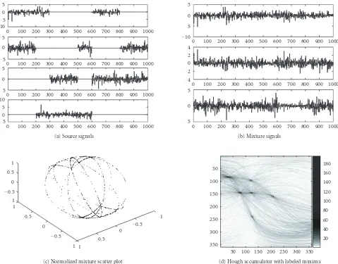
5 0 5 10 5 0 5 5 0 5 10 5 0 5

0 100 200 300 400 500 600 700 800 900 1000 0 100 200 300 400 500 600 700 800 900 1000 0 100 200 300 400 500 600 700 800 900 1000 0 100 200 300 400 500 600 700 800 900 1000

(a) Source signals

5 0 5 4 2 0 2 4 10 5 0 5

0 100 200 300 400 500 600 700 800 900 1000 0 100 200 300 400 500 600 700 800 900 1000 0 100 200 300 400 500 600 700 800 900 1000

(b) Mixture signals

1 0.5 0 0.5 1

1 0.5

0 0.5

1 1 0.5

0 0.5

1

(c) Normalized mixture scatter plot

350 300 250 200 150 100 50

50 100 150 200 250 300 350 20 40 60 80 100 120 140 160 180

(d) Hough accumulator with labeled maxima Figure4: Example: (a) shows the 2-sparse, sufficiently rich represented, 4-dimensional source signals, and (b) the randomly mixed, 3-dimensional mixtures. The normalized mixture scatter plot{x(t)/|x(t)| |t=1,. . .,T}is given in (c), and the generated Hough accumulator in (d); note that the color scale in (d) was chosen to be nonlinear (γnew:=(1−γ/max)10) in order to visualize structure in addition to the

strong maxima.

5.1. Explicit example

In the first experiment, we consider the case of source di-mensions n = 4 and mixing dimension m = 3. The 4-dimensional sources have been generated from i.i.d. sam-ples (two Laplacian and two Gaussian sequences) followed by setting some entries to zero in order to fulfill the spar-sity constraints; seeFigure 4(a). They are 2-sparse and con-sist of 1000 samples. Obviously all combinations (i,j), i < j, of active sources are present in the data set; this con-dition is needed by the matrix recovery step. The sources were mixed using a mixing matrix with randomly (uni-form in [−1, 1]) chosen coefficients to give mixtures as shown in Figure 4(b). The mixture density clearly lies in 6 disjoint hyperplanes, spanned by pairs (ai,aj),i < j, of mixture matrix columns, as indicated by the normalized scatter plot in Figure 4(c), similar to the illustration from

Figure 1(c).

In order to detect the planes in the data space, we apply the generalized Hough transform as explained inSection 3.3.

Figure 4(d)shows the Hough image withβ=360. Each

n×n-matrices where only one entry in each column differs from 0;·denotes a fixed matrix norm. In our case the gen-eralized crosstalking error is very low withE(A,A)=0.040. This essentially means that the two matrices, after permuta-tion, differ only by 0.04 with respect to the chosen matrix norm, in our case the (squared) Frobenius norm. Then, the sources are recovered using the source recovery algorithm

(Algorithm 2) with the approximated mixing matrixA. The

normalized signal-to-noise ratios (SNRs) of the recovered sources with respect to the original ones are high with 36, 38, 36, and 37 dB, respectively.

As a modification of the previous example, we now con-sider also additive noise. We use sourcesS(which have unit covariance) and mixing matrix Afrom above, but add 1% random white noise to the mixturesX=AS+ 0.01Nwhere

Nis a normal random vector. This corresponds to a still high mean SNR of 38 dB. When considering the normalized scat-ter plot, again the 6 planes are visible, but the additive noise deteriorates the clear separation of each plane. We apply the generalized Hough transform to the mixture data; however, because of the noise we choose a more coarse discretiza-tion (β= 180 bins). Curves in Hough space corresponding to a single plane do not intersect any more in precisely one point due to the noise; a low-resolution Hough space how-ever fuses these intersections in one point, so that our sim-ple maxima detection still achieves good results. We recover the mixing matrix similar to the above to get a low gener-alized crosstalking error ofE(A,A) =0.12. The sources are recovered well with mean SNRs of 20 dB, which is quite sat-isfactory considering the noisy, overcomplete mixture situa-tion.

The following example demonstrates the good perfor-mance in higher source dimensions. Consider 6-dimensional 2-sparse sources that are mixed again by matrixAwith coeffi -cients drawn uniformly from [−1, 1]. Application of the gen-eralized Hough transform to the mixtures retrieves the plane norm vectors. The recovered mixing matrix has a low gener-alized crosstalking error ofE(A,A)=0.047. However, if the noise level increases, the performance considerably drops be-cause many maxima, in this case 15, have to be located in the accumulator. After recovering the sources with this approx-imated matrixA, we get SNRs of only 11, 8, 6, 10, 12, and 11 dB. The rather high source recovery error is most proba-bly due to the sensitivity of the source recovery to slight per-turbations in the approximated mixing matrix.

5.2. Outliers

We will now perform experiments systematically analyzing the robustness of the proposed algorithm with respect to out-liers in the sense of model-violating samples.

In the first explicit example we consider the sources from

Figure 4(a), but 80% of the samples have been replaced by

outliers (drawn from a 4-dimensional normal distribution). Due to the high percentage of outliers, the mixtures, mixed by the same random 3×4 matrixAas before, do not obvi-ously exhibit any clear hyperplane structure. As discussed in

Section 4.4, the Hough SCA algorithm is very robust against

outliers. Indeed, in addition to a noisy background within the Hough accumulator, the intersection maxima are still no-ticeable, and local maxima detection finds the correct hy-perplanes (cf.Figure 4(d)), although 80% of the data is cor-rupted. The recovered mixing matrix has an excellent gener-alized crosstalking error ofE(A,A) = 0.040. Of course the sparse source recovery from above cannot recover the out-lying samples. Appout-lying the corresponding algorithms, we get SNRs of the corrupted sources with the recovered ones of around 4 dB; source recovery with the pseudo-inverse of

A corresponding to maximum-likelihood recovery with a Gaussian prior gives somewhat better SNRs of around 6 dB. But the sparse recovery method has the advantage that it can detect outliers by measuring distance from the hyperplanes. So outlier rejection is possible. Note that we get similar re-sults when the outliers are not added in the source space but only in the mixture space, that is, only after the mixing pro-cess.

We now perform a numerical comparison of the num-ber of outliers versus the algorithm performance for vary-ing noise level; seeFigure 5. The rationale behind this is that already small noise levels in addition to the outliers might be enough to destroy maxima in the accumulator thus de-teriorating the SCA performance. The same (uncorrupted) sources and mixing matrix from above are used. Numeri-cally, we get breakdown points of 0.8 for the no-noise case, and values of 0.5, 0.3, and 0.1 with increasing noise levels of 0.1% (58 dB), 0.5% (44 dB), and 1% (38 dB). Better perfor-mances at higher noise levels could be achieved by applying antialiasing techniques before maxima detection as described

inSection 4.5.

5.3. Grid resolution

In this section we will demonstrate numerical examples to confirm the linear dependence of the algorithm perfor-mance with the inverse grid resolutionβ−1_{. We consider} 4-dimensional sourcesSwith 1000 samples, in which for each sample two source components were drawn out of a distribu-tion uniform in [−1, 1], and the other two were set to zero, soS is 2-sparse. For each grid resolutionβwe perform 50 runs, and in each run a new set of sources is generated as above. These are then mixed using a 3×4 mixing matrixA

with random coefficients uniformly out of [−1, 1]. Applica-tion of the Hough SCA algorithm gives an estimated matrix

A. InFigure 6we plot the mean generalized crosstalking error

E(A,A) for each grid resolution. With increasingβthe accu-racy increases—a logarithmic plot indeed confirms the linear dependence onβ−1_{as stated inSection 4.3. Furthermore we} see that for example forβ=360, among allSandAas above we get a mean crosstalking error of 0.23±0.5.

5.4. Batch runs and comparison with hyperplanek-means

0 0.5 1 1.5 2 2.5 3 3.5

C

rosstalking

er

ro

r

0 10 20 30 40 50 60 70 80 90 100 Percentage of outliers

Noise=0%

(a) Noiseless breakdown analysis with respect to outliers

0 0.5 1 1.5 2 2.5 3 3.5

C

rosstalking

er

ro

r

0 10 20 30 40 50 60 70 80 90 100 Percentage of outliers

Noise=0% Noise=0.1%

Noise=0.5% Noise=1% (b) Breakdown analysis for varying noise level

Figure5: Performance of Hough SCA with increasing number of outliers. Plotted is the percentage of outliers in the source data versus the matrix recovery performance (measured by the generalized crosstalking error). For each 1%-step one calculation was performed; in (b) the plots have been smoothed by taking average over ten 1%-steps. In the no-noise case 360 bins were used, 180 bins in all other cases.

0 0.5 1 1.5 2 2.5 3 3.5 4

M

ean

cr

osstalking

er

ro

r

0 50 100 150 200 250 300 350 400 Grid resolution

(a) Mean performance versus grid resolution

2 1.5 1 0.5 0 0.5 1

L

o

ga

ri

th

m

ic

m

ea

n

C

ro

ss

ta

lk

in

g

er

ro

r

0 50 100 150 200 250 300 350 400 Grid resolution

In (E) Line fit

(b) Fit of logarithmic mean performance

Figure6: Dependence of Hough SCA performance (a) on the grid resolutionβ; mean has been taken over 50 runs. With a logarithmicy-axis (b), a least squares line fit confirms the linear dependence of performance andβ−1_.

three-dimensional accumulator) with k-hyperplane clus-tering algorithm (Algorithm 3). For this, random sources with T=105 _{samples are uniformly drawn from [−1, 1]} uniform distribution, and a single coordinate is randomly set to zero, thus generating 1-sparse sourcesS. In 100 batch runs, a random 4 ×4 mixing matrix A with coefficients uniformly drawn from [−1, 1], but columns normalized to 1 are constructed. The resulting mixturesX :=ASare then separated both by the proposed Hough k-SCA algorithm as well as the Bradley-Mangasariank-hyperplane clustering algorithm (with 100 iterations, and without restart).

(a) Source signals

350 300 250 200 150 100 50

50 100 150 200 250 300 350

500 1000 1500 2000 2500 3000 3500

(b) Hough accumulator with three labeled maxima

(c) Recovered sources (d) Recovered sources after outlier removal

Figure7: Application to speech signals: (a) shows the original speech sources (“peace and love,” “hello, how are you,” and “to be or not to be”), and (b) the Hough accumulator when trained to mixtures of (a) with 20% outliers. A nonlinear gray scaleγnew:=(1−γ/max)10was

chosen for better visualization. (c) and (d) present the recovered sources, without and with outlier removal. They coincide with (a) up to permutation (reversed order) and scaling.

5.5. Application to the separation of speech signals

In order to illustrate that the SCA assumptions are also valid for real data sets, we shortly present an application to audio source separation, namely, to the instantaneous, robust BSS of speech signals—a problem of importance in the field of audio signal processing. In the next section, we then refer to other works applying the model to biomedical data sets.

We consider three speech signalsSof length 2.2s, sampled at 22000 Hz; see Figure 7(a). They are spoken by the same person, but may still be assumed to be independent. The sig-nals are mixed by a randomly chosen mixing matrixA (coef-ficients uniform from [−1, 1]) to yield mixturesX=AS, but 20% outliers are introduced by replacing 20% of the samples ofXby i.i.d. Gaussian samples. Without the outliers, more classical BSS algorithms such as ICA would have been able to perfectly separate the mixtures; however, in this noisy setting, ICA performs very poorly: application of the popular fastICA algorithm [29] yields only a poor estimateAf of the mixing matrixA, with high crosstalking error ofE(A,Af)=3.73.

Instead, we apply the complete-case Hough-SCA algo-rithm to this model with β = 360 bins—the sparseness assumption now means that we are searching for sources,

the perceptual audio quality increased considerably, see also the differences between Figures7(c)and7(d), although the nominal SNR increase is only roughly 4.1 dB. Altogether, this example illustrates the applicability of the Hough SCA algo-rithm and its corresponding SCA model to audio data sets also in noisy settings, where ICA algorithms perform very poorly.

5.6. Other applications

We are currently studying several biomedical applications of the proposed model and algorithm, including the separation of functional magnetic resonance imaging data sets as well as surface electromyograms. For results on the former data set, we refer to the detailed book chapters [22,23].

The results of thek-SCA algorithm applied to the lat-ter signals are shortly summarized in the following. An elec-tromyogram (EMG) denotes the electric signal generated by a contracting muscle; its study is relevant to the diagnosis of motoneuron diseases as well as neurophysiological research. In general, EMG measurements make use of invasive, painful needle electrodes. An alternative is to use surface EMGs, which are measured using noninvasive, painless surface elec-trodes. However, in this case the signals are rather more dif-ficult to interpret due to noise and overlap of several source signals. When applying thek-SCA model to real recordings, Hough-based separation outperforms classical approaches based on filtering and ICA in terms of a greater reduction of the zero-crossings, a common measure to analyze the un-known extracted sources. The relative sEMG enhancement was 24.6±21.4%, where the mean was taken over a group of 9 subjects. For a detailed analysis, comparing various sparse factorization models both on toy and on real data, we refer to [30].

6. CONCLUSION

We have presented an algorithm for performing a global search for overcomplete SCA representations, and experi-ments confirm that Hough SCA is robust against noise and outliers with breakdown points up to 0.8. The algorithm em-ploys hyperplane detection using a generalized Hough trans-form. Currently, we are working on applying the SCA algo-rithm to high-dimensional biomedical data sets to see how the different assumption of high sparsity contributes to the signal separation.

ACKNOWLEDGMENTS

The authors gratefully thank W. Nakamura for her sug-gestion of using the Hough transform when detecting hyperplanes, and the anonymous reviewers for their com-ments, which significantly improved the manuscript. The first author acknowledges partial financial support by the JSPS (PE 05543).

REFERENCES

[1] A. Cichocki and S. Amari,Adaptive Blind Signal and Image Processing, John Wiley & Sons, New York, NY, USA, 2002.

[2] A. Hyv¨arinen, J. Karhunen, and E. Oja,Independent Compo-nent Analysis, John Wiley & Sons, New York, NY, USA, 2001. [3] P. Comon, “Independent component analysis. A new

con-cept?”Signal Processing, vol. 36, no. 3, pp. 287–314, 1994. [4] F. J. Theis, “A new concept for separability problems in blind

source separation,” Neural Computation, vol. 16, no. 9, pp. 1827–1850, 2004.

[5] J. Eriksson and V. Koivunen, “Identifiability and separability of linear ica models revisited,” inProceedings of the 4th Inter-national Symposium on Independent Component Analysis and Blind Source Separation (ICA ’03), pp. 23–27, Nara, Japan, April 2003.

[6] S. S. Chen, D. L. Donoho, and M. A. Saunders, “Atomic de-composition by basis pursuit,”SIAM Journal of Scientific Com-puting, vol. 20, no. 1, pp. 33–61, 1998.

[7] D. L. Donoho and M. Elad, “Optimally sparse representation in general (nonorthogonal) dictionaries vial1_{minimization,”}

Proceedings of the National Academy of Sciences of the United States of America, vol. 100, no. 5, pp. 2197–2202, 2003. [8] F. J. Theis, E. W. Lang, and C. G. Puntonet, “A geometric

algo-rithm for overcomplete linear ICA,”Neurocomputing, vol. 56, no. 1–4, pp. 381–398, 2004.

[9] P. Georgiev, F. J. Theis, and A. Cichocki, “Sparse component analysis and blind source separation of underdetermined mix-tures,”IEEE Transactions on Neural Networks, vol. 16, no. 4, pp. 992–996, 2005.

[10] P. V. C. Hough, “Machine analysis of bubble chamber pic-tures,” inInternational Conference on High Energy Accelerators and Instrumentation, pp. 554–556, CERN, Geneva, Switzer-land, 1959.

[11] J. K. Lin, D. G. Grier, and J. D. Cowan, “Feature extraction ap-proach to blind source separation,” inProceedings of the IEEE Workshop on Neural Networks for Signal Processing (NNSP ’97), pp. 398–405, Amelia Island, Fla, USA, September 1997. [12] H. Shindo and Y. Hirai, “An approach to overcomplete-blind

source separation using geometric structure,” inProceedings of Annual Conference of Japanese Neural Network Society (JNNS ’01), pp. 95–96, Naramachi Center, Nara, Japan, 2001. [13] F. J. Theis, C. G. Puntonet, and E. W. Lang, “Median-based

clustering for underdetermined blind signal processing,”IEEE Signal Processing Letters, vol. 13, no. 2, pp. 96–99, 2006. [14] L. Cirillo, A. Zoubir, and M. Amin, “Direction finding of

non-stationary signals using a time-frequency Hough transform,” inProceedings of IEEE International Conference on Acoustics, Speech, and Signal Processing (ICASSP ’05), pp. 2718–2721, Philadelphia, Pa, USA, March 2005.

[15] S. Barbarossa, “Analysis of multicomponent LFM signals by a combined Wigner-Hough transform,”IEEE Transactions on Signal Processing, vol. 43, no. 6, pp. 1511–1515, 1995. [16] D. H. Ballard, “Generalizing the Hough transform to detect

arbitrary shapes,”Pattern Recognition, vol. 13, no. 2, pp. 111– 122, 1981.

[17] T.-W. Lee, M. S. Lewicki, M. Girolami, and T. J. Sejnowski, “Blind source separation of more sources than mixtures using overcomplete representations,”IEEE Signal Processing Letters, vol. 6, no. 4, pp. 87–90, 1999.

[19] M. Zibulevsky and B. A. Pearlmutter, “Blind source separation by sparse decomposition in a signal dictionary,”Neural Com-putation, vol. 13, no. 4, pp. 863–882, 2001.

[20] F. J. Theis, P. Georgiev, and A. Cichocki, “Robust overcomplete matrix recovery for sparse sources using a generalized Hough transform,” inProceedings of 12th European Symposium on Ar-tificial Neural Networks (ESANN ’04), pp. 343–348, Bruges, Belgium, April 2004, d-side, Evere, Belgium.

[21] P. S. Bradley and O. L. Mangasarian, “k-plane clustering,” Jour-nal of Global Optimization, vol. 16, no. 1, pp. 23–32, 2000. [22] P. Georgiev, P. Pardalos, F. J. Theis, A. Cichocki, and H.

Bakardjian, “Sparse component analysis: a new tool for data mining,” inData Mining in Biomedicine, Springer, New York, NY, USA, 2005, in print.

[23] P. Georgiev, F. J. Theis, and A. Cichocki, “Optimization algo-rithms for sparse representations and applications,” in Mul-tiscale Optimization Methods, P. Pardalos, Ed., Springer, New York, NY, USA, 2005.

[24] R. O. Duda and P. E. Hart, “Use of the Hough transformation to detect lines and curves in pictures,”Communications of the ACM, vol. 15, no. 1, pp. 204–208, 1972.

[25] R. Dudley, Department of Mathematics, MIT, course 18.465, 2005.

[26] P. J. Rousseeuw and A. M. Leroy,Robust Regression and Outlier Detection, John Wiley & Sons, New York, NY, USA, 1987. [27] P. Ballester, “Applications of the Hough transform,” in

Astro-nomical Data Analysis Software and Systems III, J. Barnes, D. R. Crabtree, and R. J. Hanisch, Eds., vol. 61 ofASP Conference Series, 1994.

[28] A. Goldenshluger and A. Zeevi, “The Hough transform esti-mator,”Annals of Statistics, vol. 32, no. 5, pp. 1908–1932, 2004. [29] A. Hyv¨arinen and E. Oja, “A fast fixed-point algorithm for in-dependent component analysis,”Neural Computation, vol. 9, no. 7, pp. 1483–1492, 1997.

[30] F. J. Theis and G. A. Garc´ıa, “On the use of sparse signal decomposition in the analysis of multi-channel surface elec-tromyograms,”Signal Processing, vol. 86, no. 3, pp. 603–623, 2006.

Fabian J. Theisobtained his M.S. degree in mathematics and physics from the Univer-sity of Regensburg, Germany, in 2000. He also received the Ph.D. degree in physics from the same university in 2002 and the Ph.D. degree in computer science from the University of Granada in 2003. He worked as a Visiting Researcher at the Depart-ment of Architecture and Computer Tech-nology (University of Granada, Spain), at

the RIKEN Brain Science Institute (Wako, Japan), at FAMU-FSU (Florida State University, USA), and at TUAT’s Laboratory for Sig-nal and Image Processing (Tokyo, Japan). Currently, he is head-ing the Signal Processhead-ing & Information Theory Group at the In-stitute of Biophysics at the University of Regensburg and is work-ing on his habilitation. He serves as an Associate Editor of “Com-putational Intelligence and Neuroscience,” and is a Member of IEEE, EURASIP, and ENNS. His research interests include statis-tical signal processing, machine learning, blind source separation, and biomedical data analysis.

Pando Georgievreceived his M.S., Ph.D., and “Doctor of Mathematical Sciences” de-grees in mathematics (operations research) from Sofia University “St. Kl. Ohridski,” Bulgaria, in 1982, 1987, and 2001, respec-tively. He has been with the Department of Probability, Operations Research, and Statistics at the Faculty of Mathematics and Informatics, Sofia University “St. Kl. Ohridski,” Bulgaria, as an Assistant

Profes-sor (1989–1994), and since 1994, as an Associate ProfesProfes-sor. He was a Visiting Professor at the University of Rome II, Italy (CNR grants, several one-month visits), the International Center for Theoreti-cal Physics, Trieste, Italy (ICTP grant, six months), the University of Pau, France (NATO grant, three months), Hirosaki University, Japan (JSPS grant, nine months), and so forth. He has been work-ing for four years (2000–2004) as a research scientist at the Labora-tory for Advanced Brain Signal Processing, Brain Science Institute, the Institute of Physical and Chemical Research (RIKEN), Wako, Japan. After that and currently he is a Visiting Scholar in ECECS Department, University of Cincinnati, USA. His interests include machine learning and computational intelligence, independent and sparse component analysis, blind signal separation, statistics and inverse problems, signal and image processing, optimization, and variational analysis. He is a Member of AMS, IEEE, and UBM.

Andrzej Cichockiwas born in Poland. He received the M.S. (with honors), Ph.D., and Habilitate Doctorate (Dr.Sc.) degrees, all in electrical engineering, from the Warsaw University of Technology (Poland) in 1972, 1975, and 1982, respectively. He is the co-author of three international and successful books (two of them were translated to Chi-nese):Adaptive Blind Signal and Image Pro-cessing(John Wiley, 2002)MOS