Parallel hierarchical N-body methods

(1)

Thesis by John K. Salmon

In Partial Fulfillment of the Requirements for the Degree of

Doctor of Philosophy

California Institute of Technology Pasadena, California

1991

(2)

(3)

TCaHoB, ttboai

Yuk Ha Ben Finley Chris Meisl Andrea Mejia Susan Gerhart Ed Vail Bill Jones Cliff Kiser Anna Jaeckel Susan Ridgway Kim Liu Brad Scott Clo Butcher Anna Yeakley Tanya K urosky Nye Liu Bruce Bell Curtis Ling Anthony Chan Walker Aumann Alex Wei Charles Hu Dave Agabra Craig Volden Bill Gustafson Dave Kim Dan Frumin Dave Krider David Knight Bonnie Wallace

Ian Agol Dave Skeie Dawn Sumner Dawn Meekhof Brian Kurkoski Jim Bell Deepi Brar Fred Mallon Dion Hawkins Carmen Shepard Ken Hahn Di McMahon Harold Zatz Ed Llewellyn Dana Pillsbury Ken Wong Ed Naranjo Hoyt Hudson J ames Daniel Harry Catrakis Tom Wahl Erik Hille Jack Profit Jerry Carter Jesus Mancilla Viola Ng Eugene Lit Jared Smith Josh Partlow Kurth Reynolds Alice Lee Francis Ho Joe Andrieu Kevin Archie Lee Hesseltine BG Girish Greg Harry John Beahan Laura Ekroot Lisa Henderson Ben Smith Harvey Liu John Butman Lieven Leroy Matthias Blume Betty Pun Irene Chen Jung Carl 1m Lynne Hannah Nancy Drehwing Castor Fu James Shih Ken Andrews Marc Reissig N oam Bernstein Chen Yuan Jay Higley Lynn Salmon Mark Vaughan Pam Katz Rosten

Chris Chu Joe Shiang Marc Turner Mike Maxwell Peter Ashcroft Dan Kegel John Houde Mark Berman Mike Pravica Randy Levinson Dan Ruzek Karen Ross Max Baumert Nathan Inada Richard Murray Danny Chu Katy Quinn Mike Bajura Shawn Hillis Scott McCauley Dave Cole Ke-Ming Ma Mike Nygard Tim Hochberg Stefan Marelid Dave Hull Ma Blacker Mike Rigler Tim Horiuchi Stephanie Buck Davy Hull Mark Dinan Mike Serfas Tom Aldcroft Andrew Lundsten Doug Gray Matt Tyler Mike Yamada Torry Lawton Bengt Magnusson Ed Nanale Mike Nolan Mimi Zucker Tracy Ollick Eric Hassenzahl Fred Wong Mike Ricci Niel Brandt Vincent Chow Glenn Eyechaner Greg Kopp Minei Chou Paul Amadeo Alex Densmore GloryAnne Yango Jinha Kim Pa Blacker Pete Dussin Barbara Chang Imran Kizilbash John Hart Ray Banlbha Pete McCann Betina Pavri Mac Rhinelander John Wall Rob Padula Pete Wenzel Chris Cusanza Margaret Carter Kevin Kan Steve Bard Pui-Tak Kan Deron Walters Mike Guadarrama Marc Abel Steve Hwan Randy Baron Frank Lowther Nikola Pavletic Mark Huie Susan Sheu Rich Zitola James Okamoto Roderic Schmidt Matt Kidd Ted George Rob Fatland Jen Messenger Simon Goldstein Matt Penn Ted Rogers Robert Horn John Erickson Christina Garden Mike Chwe Vince Chen Robert Lord Ken Poppleton Graham Macnamara

Peter Cho Alex Rosser Ron Goodman Lushalan Liao Jennifer Johnson Po King Li Allen Price Shubber Ali Margi Pollack Mike Bronikowski Steve Lew Andy Miller Steve Gomez Mark Montague Samantha Seaward Tom Fiola Anna George Steve Hawes Marty O'Brien Sandra Blumhorst Tom Nolan Ben Holland Sylvia Chin Mike McDonald Susan Sharfstein Allan 'Wong Bill Greene Todd Walker Philip Nabors Konstantin Othmer Andrew Hsu Bill Newman Tom Megeath Randy Pollock Suman Chakrabarti Andy O'Dea Blake Lewis Tony Bladek Rodney Kinney Celina Mikolajczak

(4)

Acknow ledgments

Throughout my many years as a graduate student,

r

have been fortunate to receive support and assistance from many people and organizations. This oppor-tunity to publicly acknowledge their contributions is welcome.

First,

r

thank Professor Geoffrey Fox, my thesis advisor, for his encourage-ment and guidance during the long undertaking of this research project. During my tenure, he has provided me with an excellent working environment with the freedom to pursue topics that interest me.

Secondly,

r

thank Professor Thomas Prince, for stepping in as my advisor in the interim after Professor Fox's departure from Caltech.

r

look forward to continuing this relationship.

The work described in this thesis was the result of a fruitful collaboration.

r

certainly could not have done it without Peter Quinn, Wojciech Zurek, Craig Hogan and especially Mike Warren, who spent many, many hours helping with the development, testing, debugging and running of the parallel BH code.

r

am indebted to Joshua Barnes for making his implementation of the al-gorithm available, in source code form, to the astrophysics community, myself included.

None of this work would have been possible without the staff which created and maintained a superb computational environment. Thanks to Chip Chapman, Heidi Lorenz-Wirzba, Mark Beauchamp, Charles DeBardeleben, Hiram Hunt, Doug Freyberger.

r

would also like to thank Mary Maloney and Terry Arnold for keeping the red tape at bay.

(5)

Williams, Steve Otto, David Walker, Jeff Goldsmith, Sun Ra, Paul Stolorz, Clive Baillie and James Kuyper.

Throughout my stay at Cal tech, I have been the recipient of generous financial support. The Shell Foundation supported me with a graduate fellowship. In addition, this work was supported by the National Science Foundation, and the Departement of Energy.

Very special thanks must go to the members of Blacker House for "engaging me in varied and interesting conversation."

(6)

Abstract

Recent algorithmic advances utilizing hierarchical data structures have resulted in a dramatic reduction in the time required for computer simulation of N-body systems with long-range interactions. Computations which required

O(N2)

oper-ations can now be done in

O(N

log

N)

or

O(N).

We review these tree methods and find that they may be distinguished based on a few simple features.

The Barnes-Hut (BH) algorithm has received a great deal of attention, and is the subject of the remainder of the dissertation. We present a generalization of the BH tree and analyze the statistical properties of such trees in detail. We also consider the expected number of operations entailed by an execution of the BH algorithm. We find an optimal value for m, the maximum number of bodies in a terminal cell, and confirm that the number of operations is

O(N

log

N),

even if the distribution of bodies is not uniform.

The mathematical basis of all hierarchical methods is the multipole approxi-mation. We discuss multipole approximations, for the case of arbitrary, spherically symmetric, and Newtonian Green's functions. We describe methods for comput-ing multipoles and evaluatcomput-ing multipole approximations in each of these cases, emphasizing the tradeoff between generality and algorithmic complexity.

(7)

(8)

List of Figures

An example of Appel's hierarchy of clumps. . . . The binary tree representation of an Appel hierarchy. Expanded representation of a BH tree.

Flat representation of a BH tree . . .

Representation of the hierarchy of levels in Greengard's method. Earth-Sun system . . . .

Iterative construction of BH tree. Iterative construction of BH tree. Iterative construction of BH tree. Iterative construction of BH tree.

<

Pop>

vs.

A, . . . .

<

Pop>

1m

vs.

A,/m.

Cavg vs. N . .

mCaV9 N

- N - vs .

Davg vs. N.

mSDa"9 N

N vs.

One dimensional pathological BH tree. Labeling of regions around

V,.

Labeling of regions around

V,.

Boundary effects in estimating Pmid.

(Nbb) INm VS. N. K1(a,(3)

IVK

1(a,(3)1

K2(a,(3)

IVK

2(a,(3)1 K4(a,(3)

(13)

5.6

5.7

5.8

5.9

5.10 5.11

5.12

5.13

5.14 5.15 5.16 6.1 6.2 6.3

6.4

6.5 6.6

6.7

7.1

7.2

7.3

7.4

7.5

7.6

7.7 7.8 7.9

Geometry used in K~up computations. Contour of

K;UP(r)

= 0.01

Contour of

K;UP(r)

= 0.1 Contour of

KtUP(r)

= 0.1

1~<p~(4)(e)))1

l~a~(4)(e)))1

(( <p;(2)(e)))

~

122 124 126

127

128

140 141

142

((la~(2)(e)12)) ~

(( <p;(3)(e)))

~

. . .

143

((la~(3)(e)12)) ~

A two-galaxy system.

Pathological situation for BH DpeningCri terion.

Worst case situation arising from BH DpeningCri terion. Geometry of Vmid with the original BH DpeningCri terion.

Geometry of Vmid with the (edge, Cart) DpeningCri terion.

Foe vs.

e

Equivalent values of

e

for different opening criteria An ORB domain decomposition . .

A one-dimensional decomposition A Gray code decomposition Domain Decomposition. A two-galaxy system.

Menwry and processor domain geometry A two-galaxy system with long-dim splits Data flow in a 16 processor system. Illustration of FindParent

(14)

7.10

7.11

8.1

8.2

8.3 8.4 8.5 8.6

8.7

8.8 8.9 8.10

8.11

8.12

8.13 8.14 8.15 8.16

Illustration of DomainOpeningCri terion. False positive from DomainOpeningCri terion

T step vs. Number of processor. Tforce vs. N

Speedup vs. Number of processor. Total overhead vs. Ngrain.

Copied memory overhead, gcopy vs. Ngrain

Imbalanced memory overhead, gimbal vs. Ngrain Ngrain vs. maxC dstep )

Simplified interaction domain of a processor Memory/ Ngrain vs. natural grain size, q.

Complexity overhead, fcplx vs. Ngrain. .

Complexity time, Tcplx vs. copied memory, Mcopy.

Complexity overhead, Nindcplx vs. natural grain size, q. Waiting overhead, fwait vs. Ngrain.

209

210

223

225

228

230

232

233

235

236

239

241

244

245

247

Empirical fit for waiting overhead, fwait *Nint vs. natural grain size, q.249

l082(Nproc )

Communication overhead, fcomm vs. Ngrain.

Load imbalance overhead, Jimbal vs. Ngrain . .

(15)

1. Hierarchical Techniques and N-body

Simula-tions

Physical systems may be studied by computer simulation in a variety of ways. Simulations with digital computers are constrained by factors associated with the finite speed of computation and the finite size of the computer. Generally, these factors require that the first step in any computer simulation of a physical phe-nomenon be to develop a mathematical model of the phephe-nomenon consisting of a finite number of discrete parts. The correspondence between the discrete compo-nents in the computer simulation and the physical phenomenon itself is completely arbitrary, limited only by the imagination of the scientist.

Often, the discretization is arrived at indirectly, by means of partial differen-tial equations. First, one models the physical system by a set of pardifferen-tial differendifferen-tial equations. Then, one applies techniques of discrete approximation such as finite difference methods or finite element methods to recast the mathematical problem into a discrete form. An alternate, and less widely used, approach is to discretize the physical system into a finite set of "bodies" or "particles" which interact with one another as well as with externally applied "forces." The bodies carry some state information which is modified as the simulation proceeds, according to the interactions. Simulations based on this type of discretization are referred to as "N-body" simulations. Hockney and Eastwood[l] have extensively reviewed the techniques of N-body simulations, as well as applications in plasma physics, semi-conductor device simulation, astrophysics, molecular dynamics, thermodynamics and surface physics. Applications also exist in fluid mechanics,[2, 3, 4] applied mathematics,[5] and undoubtedly other areas as well.

(16)

consist of a position and a velocity, and the interaction between bodies is a model for some kind of force law. The dynamical state of the system is evolved by alter-nately adjusting the velocities based on accelerations that result from interparticle interactions, and the positions, based on the velocities.

1.1.

Categories of N-body sinlulations.

In their monograph, Hockney and Eastwood[l] classify N-body methods broadly into three categories:

1. Particle-Particle (PP) methods. 2. Particle-Mesh (PM) methods.

3. Particle-Particle Particle-Mesh (PPPM or

p

3_{M) methods.}

We briefly review these methods to provide context for the discussion of tree methods which follows.

1.1.1. PP methods.

In PP methods, particles interact directly with one another. The basic control structure, which is repeated over and over as the simulation proceeds, is outlined in Codes 1.1 and 1.2.

ComputeAlllnteractions

for(each body, b)

Computelnteraction(of b with all other bodies)

endfor

for(each body b)

UpdatelnternaIState(b)

endfor

endfunc

Code 1.1. Function to compute all pairwise interactions among a set of bodies.

(17)

ComputeInteraction(b)

for(each body, bj 3 bj -=1= b )

PairInteraction(b, bj )

endfor endfunc

Code 1.2. Function to compute all interactions with a particular body, b.

bodies. The simplicity of Codes 1.1 and 1.2 allows for straightforward expression in a suitable computer language like C or FORTRAN. The simplicity also allows one to easily take advantage of "vectorization," whereby the full power of modern supercomputers can be efficiently used. Parallelization is also reasonably straight-forward,[6] making it possible to use large parallel computing systems which de-rive their speed and cost-effectiveness from the assembly of numerous modest, autonomous processors into a single parallel system.

The most significant drawback of PP methods is their scaling for large num-bers of bodies. An implementation following Codes 1.1 and 1.2 requires each body to interact with every other body in the system. Each time Code 1.1 is executed, the function Pairlnteraction is called N(N -1) times, where N is the number of

bodies in the simulation. Even if Code 1.2 is modified to take advantage of a com-mutative interaction, i.e., one for which Pairlnteraction(b1 , b2 ) is equivalent to

Pairlnteraction(b2 , b1 ), then Pairlnteraction is executed only half as many times. Unfortunately, this does little to mitigate the rapid growth, proportional to N2

•

If the interaction between particles is short-range, then Code 1.2 can be re-placed with Code 1.3. The loop in Code 1.3, which is restricted to bodies in a ball of radius rcut around b, requires computation of only Nneigh pair interactions,

where N neigh is the number of bodies in the ball. For homogeneous systems, Nneigh is of 0(1), i.e., independent of N. Hockney and Eastwood describe data

structures which allow one to select the Nneigh neighbors in a ball of fixed radius

(18)

Code 1.1 requires only O(N N Neigh) executions of Pairlnteraction. Of course, if

Nneigh is very large, this may be little improvement over the the O(N2) behavior of Code 1.2.

If the interaction does not have a natural distance cutoff, PP methods are limited to situations in which N

<

few x 104.

CornputeShortRangelnteraction(b)

for(each body bj ::1 Separation(b, bj)

<

Tcut)

Pairlnteraction(b, b_{j )}

endfor endfunc

Code 1.3. An alternative form of Cornputelnteraction, applicable when the interaction is negligible beyond a distance of Tcut.

1.1.2. PM luethods.

PM methods offer the advantage of O(N) behavior for large N, even if the interac-tion cannot be neglected outside of some distance cutoff. However, they introduce approximations which may be problematical. PM methods are applicable when the interaction is expressible as the solution of a differential equation, discretized onto an auxiliary mesh. Electromagnetic and gravitational interactions have this property, with

(1.1 )

(1.2)

(19)

methods,[7, 8] which converge in time O(Nmesh ), with a remarkably small con-stant of proportionality, where N mesh is the number of grid points in the discrete

mesh.

Hockney and Eastwood discuss the relationship between Nand N mesh .

Gen-erally speaking, the two should be roughly comparable. Otherwise, laboriously obtained information is thrown away each time one moves back and forth between the mesh representation and the body representation.

The approximation introduced by the PM method generally results in de-pressing the strength of short-range interactions. The interaction between any bodies whose separation is less than a few mesh spacings will be significantly re-duced from the PP case. In some circumstances, this "error" actually results in the simulation more faithfully representing the physical phenomena, e.g., collision-less plasmas. In any event, PM methods can only model phenomena on length scales larger than a few mesh spacings. Thus, the smallest interesting length scales dictate the required mesh spacing. If the system under study is highly inhomoge-neous, with length scales extending over a few orders of magnitude, then the size of the mesh may become prohibitive.

1.1.3. PPPM methods.

Finally, Hockney and Eastwood discuss PPPM methods. These methods attempt to recover some of the accuracy lost by PM methods without reintroducing the O( N2

) behavior of PP methods. In essence, a carefully designed short-range

inter-action is computed by PP methods, as in Code 1.3. This additional force is added to the usual PM interaction. The short-range component is an analytic approxi-mation to the error introduced by the PM method. Since the error introduced by the PM method is of limited range, i.e., a few mesh spacings, the correction may be computed using Code 1.3 in time O(N Nneigh).

(20)

N, then Nneigh may be a significant fraction of N, leading to O(N2) behavior,

albeit with a much smaller constant of proportionality than simple PP methods. Furthermore, the great simplicity of Code 1.2 which facilitated efficient vectoriza-tion and parallelizavectoriza-tion is lost for PPPM techniques. Although still possible, it requires considerably more effort to vectorize or parallelize a PPPM method.

1.2. Tree lnethods

Since Hockney and Eastwood's monograph was published, an entirely new class of particle simulation methods has emerged as an alternative to PP, PM or PPPM methods. These methods are characterized by an organization of particles into a hierarchy of clusters, which span the full range of length scales from the minimum interparticle spacing up to the diameter of the entire system. These methods are usually referred to as "tree methods" or "hierarchical methods" because of the data structures which are used.

1.2.1. Appel's m.ethod.

(21)

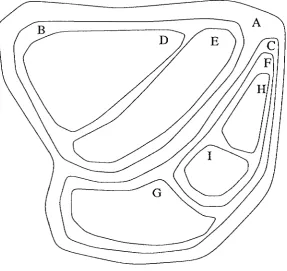
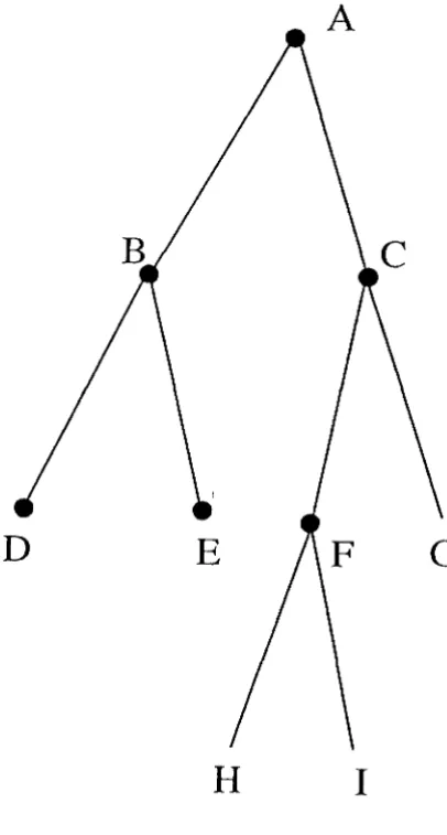
In Appel's terminology, bodies are collected into "clumps," which in turn are collected into larger clumps, and so on. The resulting data structure is a binary tree. Of course, there are many binary trees that can be constructed from a collection of bodies. A good tree will collect physically nearby bodies within the same branch. Figure 1.1 illustrates how a region of space might be divided into clumps which represent amorphous regions of space. Figure 1.2 shows the binary tree equivalent to the hierarchy of clumps shown in Figure 1.1. Of course, even given the constraint that clumps should correspond to compact regions of space, there is still a great deal of freedom in the choice of hierarchy. Appel builds the tree in two steps:

1. Build a "k-d tree" with the property that the bodies contained within the two descendants of a given node are separated by a plane parallel to one of the Cartesian axes, and have equal numbers of bodies. In other words, the left child contains all bodies below the median coordinate, and the right child contains all bodies above the median. The coordinate, i.e., x, y or z, alternates at successive levels of the tree.

2. Refine the tree, so that the nearest external clump to any clump is its parent. This is achieved with a local modification procedure that Appel calls a "grab." He points out the effectiveness of the "grab" procedure is difficult to analyze. Once the tree is built, the acceleration of each clump is calculated by a re-cursive descent of the tree. Each node of the tree, i.e., each clump, only stores velocities and accelerations relative to its parent. The acceleration of a clump rela-tive to its parent is due solely to the influence of its sibling. Thus, the acceleration of all the nodes in the tree can be computed by applying the recursive procedure, ComputeAccel, shown in Code 1.4, to the root of the tree.

(22)

(23)

H

I

(24)

ComputeAccel(node)

ComputeAccel(RightChild(node»

ComputeAccel(LeftChild(node»

Interact (RightChild(node) , LeftChild(node»

endfunc

Code 1.4. Appel's algorithm for computing the acceleration of a node in a tree.

Interact(A, B)

Larger

=

larger of A and B

Smaller

=

smaller of A and B

if( Diameter(Larger)

>

8

*

Separation(A, B) ) Interact (RightChild(Larger) , Smaller);

Interact (LeftChild(Larger) , Smaller);

else

Monopole(Larger, Smaller);

Code 1.5. Appel's algorithm for computing the interaction between two nodes in a clustering hierarchy. If the nodes are sufficiently well

sepa-rated, then a monopole approximation is used. Otherwise, the

interac-tions between their components are individually computed.

The parameter 8 may be freely varied between 0 and 1. When 8 equals

zero, every pair of bodies interacts, in much the same way as in Code 1.2. For

fixed, non-zero values of 8, Appel estimates the number of evaluations of the

subroutine Monopole to be

O(N logN),

but Esselink [11] has shown that Monopole

is actually executed only

O(N)

times. Esselink's arguments are rather involved.

The following simple discussion illustrates why Appel's algorithm is

O(N):

1. The nature of the recursion in Code 1.5 guarantees that clumps which

inter-act via Monopole, are approximately the same size. The reason is that the

recursive call to Interact always subdivides the larger of the two clumps. Its

(25)

from the smaller sibling.

2. Consider a particular clump, C. The clumps with which it interacts VIa Monopole are more distant than its size times 8-1

, and less distant than its size times 28-1_. _If_{they were more distant than}_28-1_,_{then they would have} interacted with C's parent.

Assuming these two premises are valid, we conclude that the volume available for the clumps with which C interacts is limited to some fixed multiple of C's volume, while the clumps themselves are not smaller than some other fixed multiple of C's volume. Thus, there can be at most, 0(1) such clumps, independent of N.

Since there are 2N -1 clumps in a binary tree with N terminal nodes, and each is an argument to Monopole only 0(1) times, the total number of calls to Monopole must be O(N).

Appel's algorithm has not been widely adopted. Appel himself recognized that the imposition of a hierarchical data structure on the physical system, and its associated approximations, might lead to non-physical, hierarchical artifacts in the final result. This would be highly undesirable in circumstances where the purpose of the simulation is to study the evolution of some physical clustering phenomenon, e.g., the growth of structure in the universe.[12] Furthermore, the somewhat chaotic and tangled structure of the binary tree after the application of the "grab" procedure makes the accuracy of the method difficult to analyze precisely. Finally, the restriction to the very crude monopole approximation re-quires a low value of 8, and a large number of executions of Monopole in order to achieve acceptable accuracy. It is possible, however, to adapt Greengard's[13] or Zhao's[14] formalism for higher order multipoles into Appel's framework.[15]

1.2.2. Barnes and Hut's Ill.ethod

(26)

larger one in half along each of the three coordinate axes. In Appel's terminology, each such cube represents one "clump," with size given by the length of an edge. We shall call these cubes "cells." In addition, the tree structure is recomputed, ab

initio for each iteration; there is nothing analogous to the "grab" procedure. The second important difference is that BH compute accelerations only for bodies. The internal nodes of the tree are not dynamical objects that influence one another. They are merely data structures used in the computation of the forces on the bodies. In fact, it is possible to compute accelerations for arbitrary test bodies; even ones which are not included in the tree.

Finally, BH suggest, and Hernquist[18] elaborates upon the possibility of in-cluding quadrupole and higher order terms in the force calculation.

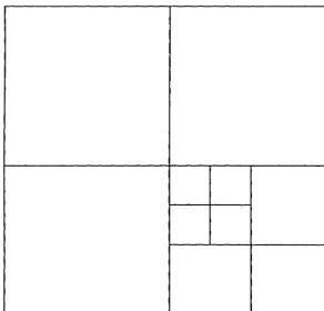
An example of the tree used by BH is shown in Figure 1.3. For simplicity, we shall usually render trees and other data structures as though we were considering two-dimensional simulations. The generalization to three dimensions is obvious. The figure makes clear the hierarchical nature of the structure, with each internal "node" or "cell" having exactly four descendants, each of exactly half the linear size of the parent. In three dimensions, of course, each cell has eight descendants. The root of the BH tree corresponds to the entire computational volume, i.e., it encompasses all of the bodies in the N-body simulation. As we shall see, the terminal nodes correspond to regions that contain one body. Thus, the BH tree contains groupings of objects over the entire range of length-scales present in the simulation. The tree is "adaptive" in the sense that it naturally extends to more levels in regions with high particle density and short length-scales.

(27)

(28)

presence.

The BH algorithm proceeds as follows:

1. Build a BH tree with the property that each terminal node has exactly zero or one body within it.

2. Compute the mass and center-of-mass of each internal cell in the tree. Record this information so that each internal cell may be treated in Code 1.6 as a body with a mass and position.

3. For each body, traverse the tree, starting at the root, using the procedure in Code 1.6.

ComputeField(body, cell) if( cell is terminal)

Monopole(body, cell)

else if( Distance(cell, body)

>

e

*

Size(body» fore each child of cell )

ComputeField(body, child) endfor

else

Monopole(body, cell) endif

endfunc

Code 1.6. Function ComputeField computes the interaction between a specified body, and all bodies lying in a cell.

As we shall see in Chapter 4, when ComputeField is called for every body in the tree, Monopole is executed

O(N

log

N)

times.

The BH algorithm can be generalized in several ways.

1. The tree can be constructed with a terminal-size parameter, m. Terminal nodes are required to have m or fewer bodies. BH consider m = 1. We consider the effect of m

i=-

1 in Chapters 2 and 4.

(29)

(30)

a function that computes both monopole and quadrupole interactions. [18, 17, 19,20]

3. The form of the interaction need not be Newtonian gravity. In Chapters 3, 4 and 5, we consider the applicability of the BH algorithm to other forms of interaction.

4. The form of the opening criterion, i.e., the predicate which determines whether the multipole approximation will be used for a given body and cell, may be modified. In addition to adjusting the parameter (), one can contemplate alternatives which are both faster and more accurate. This topic is considered in Chapter 6.

5. It is possible to reformulate the algorithm to take advantage of "vector" su-percomputers.[21, 22, 20]

6. The BH algorithm can be reformulated to take advantage of parallel computer hardware. This is discussed in Chapters 7 and 8.

1.2.3. Greengard's method.

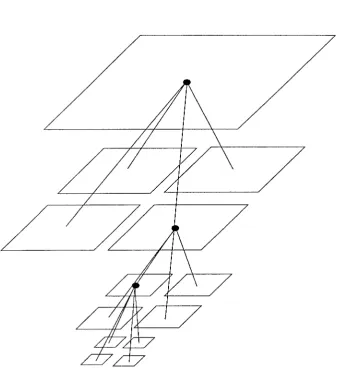
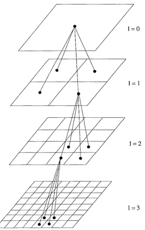
Another algorithm has been introduced by Greengard and Rokhlin.[13, 23, 24] Greengard combines feature of Barnes' as well as Appel's formulation, and develops an extensive formalism based on spherical harmonics. As in Appel's method, accelerations are computed between internal nodes of the tree, leading to an overall time complexity of O(N). On the other hand, the cells in the hierarchy are cubes which fill space completely, as in the BH method. Greengard has presented his algorithm in a static, rather than an adaptive form. The hierarchy in Greengard's method is a set of grids, each with twice as many cells in each direction as the layer above it. The structure is shown in Figure 1.5. With a representation of the data as in Figure 1.5, Greengard's method is not adaptive. The finest level of the hierarchy samples the system at the same level of detail, throughout the computational volume.

(31)

1=0

1

=

1

1=2

1=3

(32)

each cell interacts with 875 = 103 - 53 nearby cells at the same level of the tree. Instead, Greengard controls errors by expanding the mass distribution in each cell to a fixed number of multipoles. He makes an extremely strict accounting of the errors introduced by approximating a distribution by a 2P-pole multipole

expansion, and concludes that the fractional error, E, is bounded by

(1.3)

Hence, he concludes that to obtain results accurate to within E, one should carry out the expansion with

(1.4 )

Greengard develops an extensive formalism for manipulating coefficients of spherical harmonics. The basic "interaction" in Greengard's algorithm consists of the translation of a multipole expansion from one center to another. For all but the simplest situations ("\vhich corresponds to the Monopole clump-clump interactions in Appel's algorithm) this is an extremely complex operation, requiring evaluation of high-order spherical harmonics and some p4 floating point operations. Thus,

despite its extremely promising O(N) asymptotic behavior, the constant of pro-portionality which relates time to N is very large. Greengard estimates that some

875p4 N operations (some of them evaluations of high-order spherical harmonics) are required to compute potentials for N bodies. Greengard does not discuss the additional complexity needed to compute forces, except to remark that the gradients of the spherical harmonics may be computed analytically.

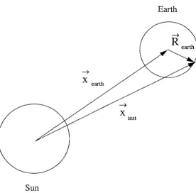
1.2.4. An illustrative example.

(33)

~

X earth

Sun

Figure 1.6. Earth-Sun system.

~

X

test

(34)

Appel would consider both the Earth and Sun to be "clumps" located at their respective centers-of-mass. The acceleration of all of the Earth bodies (neglecting interactions between pairs of Earth bodies) would be the same, given by

(1.5)

In particular, there would be no tides, which arise from the difference between the Sun's gravitational attraction on the daytime and nighttime sides of the Earth.

If tides are important, Appel would recommend decreasing 0 so that,

Diameter(Earth)

>

oSeparation(Earth, Sun),

(1.6)

in which case the Earth would be subdivided into two or more sub-clumps before the monopole approximation was made. This would also have the effect of re-quiring subdivision of the Sun into many earth-sized clumps, each of which would require its own monopole interaction. Of course, there is no guarantee that the Earth would be split into the "correct" sub-clumps. They are as likely to be the Northern and Southern Hemispheres as to be Night and Day. Thus, the only safe procedure is to set

o

<t::

Diameter( Earth) / S eparation( Earth, Sun).

(1.7)

Such a small value of 0, would, of course imply a very large number of executions of Monopole.

(35)

Finally consider Greengard's method. Again the mass distribution of the Sun is approximated, but now many terms (perhaps up to 210_pole) in the multipole expansion are retained. Of course, since the Sun is almost spherical, the magni-tudes of most of the high-order terms would be very small. The field from the Sun is "translated" to the center of the Earth resulting in a new multipole expansion about the center of the Earth. The familiar solar tides arise from the contribution of the Sun's monopole term to the quadrupole term in the expansion about the center of the Earth. If we consider only the monopole term from the sun, then Greengard's formalism tells us

GMsun 2

(4;

°

-I~

131R earthl

VS

Y2(B,</J)+""

Xearth

(1.8)

where Yim are the spherical harmonics, B is the angle between Rearth and Xearth.

The azimuthal angle, </J, happens to be irrelevant in this case. Greengard does not compute explicit error bounds for the gradient of </J, but we may compute it analytically as:

~

) GMsun

~

(I

1

ff7r

0 )

-'\1</J(Xtest = - ~ 2'\1 Rearth - Y1 (B,</J)

IXearth 1 3

+ GMsun

V

(IR

12

(4;

yO(B

A.))

1

Xearth ~

1

3 earth

V

S

2 , If'

(1.9)

The first term in Eqn. 1.9, gives rise to the usual acceleration of all Earth parti-cles uniformly toward the Sun, while the second gives the tidal variations, which depend on the angle

e.

1.2.5. Other tree rn.ethods.

(36)

Jernigan and Porter[25, 26, 27] describe a method which treats the hierarchy as a dynamical object, in which the velocity and acceleration of a node in the tree is always with respect to its parent. They use a binary tree similar to Appel's. In order to improve on the accuracy of Appel's method, they transform the equations of motion for each pair of siblings into a "regularized" form.

Pepin, Chua, Leonard, and Winckelmans[15, 28] have described yet another hierarchical method. The simulation of interacting "vortex particles" as mod-els of fluid flow shares the same long-range difficulties as gravitational N-body simulations. They use a binary tree, similar to that used by Appel, and a mul-tip ole expansion similar to Greengard's two-dimensional formalism. Pepin has shown that the method can be parallelized, achieving good efficiency on up to 32 processors.[15] This work specifically treats two-dimensional problems, for which Greengard's formalism is considerably simplified. In principle, three-dimensional problems may be treated by adopting either Greengard's or Zhao's formalism for translation of three-dimensional multipoles.

Zhao[14] has described an O(N) algorithm that is very similar in structure to Greengard's method. The difference lies in the representation of the multipole expansion. Where Greengard uses a formalism based on spherical harmonics, Zhao uses a formalism based on Taylor series and Cartesian coordinates. Otherwise, the structure of the algorithms is identical. Zhao and Johnsson[29] have demonstrated that the algorithm may be adapted for execution on the Connection Machine, a SIMD system with 65536 single-bit processors and 2048 floating point units. Their results are only for uniform distributions of bodies. They do not consider problems of load balancing or implementation of adaptive hierarchies.

Katzenelson[30] presents a unified framework which encompasses both Green-gard's algorithm and a non-adaptive version of Barnes' algorithm, as well as an outline for implementation on the Connection Machine. He also does not con-sider the problem of load balance or the need for adaptive structures when the distribution of bodies in space is highly non-uniform.

(37)

method with similarities to Appel's method and BH. As in Appel's method, the hierarchy is constructed as a binary tree. The construction is slightly different, however, based on a technique for finding "mutual nearest neighbor" pairs. This technique seems to eliminate some of the uncertainties associated with Appel's "grab" procedure. The force calculation now proceeds in a manner very similar to the BH algorithm. The tree is traversed once for each body, applying an opening criterion at each node which determines whether the quadrupole approximation is adequate, or, conversely, whether the interaction must be computed with the daughters of the node. The method requires O( N log N) executions of the basic quadrupole interaction subroutine to compute forces on all bodies. Makino [20] has found that the force evaluation is approximately as time-consuming as the BH algorithm, for a given level of accuracy, but the construction of the tree takes roughly ten times as long.

1.3. Categorization of tree lllethods.

Obviously, a large number of tree methods have been suggested, with diverse scalings, data structures, mathematical foundations, etc. Nevertheless, many also share features in common. Table 1.1 categorizes the different methods according to the following criteria:

Tree type: The methods use either binary trees or octrees. The octrees are generally easier to construct, as they do not require searching for neighbors, computing medians, etc. Since they do not impose any external rectangular structure, the binary trees may introduce fewer artifacts into the simulation. There is little evidence one way or the other.

Multipoles formalism: Methods make use of monopole, quadrupole or arbitrarily high order multipoles. When high order methods are used, they are either based on spherical harmonics or Taylor series expansions.

Adjustable opening criterion: Some methods have an adjustable parameter, e.g.,

B, which controls the opening of nodes in the tree during traversals.

(38)

levels in regions in which bodies are present with high spatial densities. In

general, those methods which are not adaptive can be made so by altering the

fundamental data structure from an "l-D array of 3-D arrays" to an octree. Scaling: The methods are either O(N log N) or O(N). As logN grows so slowly

the difference between the asymptotic speeds for very large N may be of little

practical significance. For practical values of N, the "constants" are at least

as important as the functional form of the scaling.

Interaction type: Some of the methods compute interactions between nodes of

the hierarchy, while others only compute interactions between isolated bodies

and nodes of the hierarchy. All methods compute some interactions between

pairs of bodies. The methods which allow nodes to interact have a scaling

behavior of O(N), while those which have only body-node interactions scale

as O(N log N). Generally, node-node interactions are extremely complex.

We distinguish between the different algorithms based on the most complex

type of interaction allowed, i.e., either body-body (B-B), body-node (B-N) or

node-node (N-N).

Table 1.1. Classification of tree methods according to criteria described in the text.

Appel BH GR Zhao Pepin Benz JP

Binary fOct-tree B

0

B B B

Multipoles Mono Quad Sphr. Tayl. Sphr. Quad Mono

Adjustable OC Yes Yes No No Yes Yes Yes

Adaptive Yes Yes No No Yes Yes Yes

Scaling N NlogN N N N NlogN NlogN

Interactions

Jr-If

B-N N-N N-N N-N B-N B-N

AI-tJ

1.4. Outline of dissertation.

The remainder of this dissertation will be concerned with various aspects of the

BH algorithm. \iVe concentrate on the BH algorithm for several reasons:

(39)

will likely be the most reliable algorithm for use in "real" scientific simulations. 2. Joshua Barnes kindly provided a copy of his version of the code which was written in the C programming language, facilitating portability to Caltech's parallel computers.

3. The firm distinction between the force calculation and the tree construction phase makes effective parallelization much easier. Although by no means im-possible to parallelize, Appel's and Greengard's algorithms require consider-ably more bookkeeping because of the need to store and compute interactions for non-terminal objects in their hierarchies. It is likely that load balance ,vill be considerably harder for either of these algorithms, in comparison to BH. 4. The asymptotic rates,

O(N

log

N)

vs.

O(N),

do not tell the whole story.

Based on Greengard's estimate of 1752N pair interactions per time-step[13] (pg. 70-71), and our empirical observation that the BH algorithm with

B

= 0.8 requires approximately 15-35

N

log2

N

pair interactions per timestep, the asymptotic regime in which Greengard's algorithm is expected to be su-perior is near N ~ 1015

- well beyond any planned simulations. It is worth noting that the exact value of the crossover point depends exponentially on the precise constants that precede the

O(N

log

N)

and

O(N)

factors. The turnover point can be changed by many orders of magnitude by relatively small adjustments in parameters or algorithms.

(40)

(41)

2. Properties of the

'"

H Tree.

In this chapter we investigate some statistical properties of the BH tree. Such

quantities as the average depth of the tree and the number of non-terminal nodes will be important in the discussions of performance, so we begin by studying the

tree itself.

2.1. Building the tree.

We define a generalized BH tree by the following properties:

1. The cells partition space into an octree of cubical sub-cells, so that each cell has eight descendants of equal size.

2. No terminal node of the tree contains more than m bodies. BH consider the

case, m = 1.

3. Any node of the tree which contains m or fewer bodies is a terminal node, i.e., it is not further subdivided.

There are many ways to construct such a data structure from a list of bodies.

One method is to begin with an empty tree and to examine each body in turn, modifying the tree as necessary to accommodate it. To add a body, it is necessary

to find the most refined element of the current tree which contains the body, and

then to add the body directly to that element, either by refining it further or by

simply inserting the body. Barnes describes a recursive procedure which performs

the above steps. In the following code fragments, we will encounter two distinct data types:

Bodies: These contain a position, a mass, a velocity, and perhaps other physical data which is carried by the bodies in the simulation.

Cells: These represent cubical volumes of space. Cells which are internal have

(42)

terminal.

Cells may be further subdivided into two types:

Internal Cells: These are the internal nodes of the BH tree. Each Cell contains

a set of multipoles which may be used to approximate the effect of all the

bodies which are descendants of the cell. In addition, a Cell contains pointers

to up to eight direct descendants.

Terminal Cells: These are the terminal nodes of the BH tree. As we shall see

in Chapter 4, if m is chosen correctly, then terminal cells need not store a

multipole expansion. They simply store the header for a linked list of bodies

and enough information to specify the size and location of the region of space

enclosed by the cell.

Insert(Body, Cell)

if( Cell is not terminal )

if( Cell has a Child which encloses Body)

Insert (Body, Child)

else

NewChild(Body, Cell)

endif

else if( Cell contains fewer than m bodies )

InsertDirectly(Body, Cell)

return;

else if( Cell contains exactly m bodies)

NewCell=a new, non-terminal cell with

eight empty children

fore oldbody = each body in Cell )

Insert (oldbody, NewCell)

endfor

Insert (Body, NewCell)

replace Cell with NewCel1

endif

endfunc

(43)

•

Ie

•

(44)

•

..

•

~

•

(45)

•

w

~

•

..

•

~

•

• •

•

(46)

•

Figure 2.4. Snapshot of an m inserted using Code 2.1.

•

~

•

~

~ t

..

•

Ia

•

~

•

(47)

The function Insert in Code 2.1 is essentially equivalent to Barnes' method of inserting a body into a cell. The function InsertDirectly, which is used by Insert, simply adds a body to the list of bodies associated with a terminal cell. The function NewChild, creates a new terminal node which contains only one Body, and links it into the tree as a child of Cell.

Figures 2.1 through 2.4 show the evolution of a two-dimensional tree built ac-cording to the method of Code 2.1. Notice that the sequence shown in these figures would be very different had we inserted bodies in a different order. Nevertheless, the tree that finally results from this procedure is unique.

Once the tree is in place, the centers-of-mass and multipole moments of each of the internal nodes can be computed using a general form of the parallel axis theorem. We will consider multipole moments and the parallel axis theorem in some detail in Chapter 4. We now turn to the statistical properties of the tree itself.

2.2. Notation.

We begin with a finite cubical volume,

Va,

representing all of space, i.e., no body falls outside of this volume, and an underlying probability density function p(x).

Now consider a collection of N coordinates (or bodies), {Xl, ... ,X N }, independent, identically distributed random variables, with probability density

p( x).

We are in-terested in statistical properties of the BH tree constructed from these bodies. For example, how deep is it, how many internal nodes does it contain, and how many operations are entailed by an application of the BH force calculation algorithm, on average?

We begin with some notation. We shall label cubical cells with a subscript ,. Every possible cell is labeled by some, - those which are in the BH tree, as well as those which are not.

(48)

ancestors. We note that all cells at the same depth have the same volume,

V -_{i -} Vr 8-d(i)

0 ,

(2.1)

and there are 8d cells with depth equal to d. We define Ld as the set of cells at level d, i.e.,

(2.2)

For any cell, Pi is the probability that a particular body lies within Vi'

(2.3)

The probability that Vi will contain exactly z bodies is given by the binomial distribution function,

(2.4)

We also define the cumulative binomial distribution and its complement, m

CN,m(Pi) = LBN,j(Pi) (2.5)

j=O

and

N

DN,m(Pi) = 1 - CN,m(Pi) = L BN,j(Pi)' (2.6)

j=m+l

The functions, Cm,N and Dm,N are related to the incomplete beta function.[34] For two disjoint volumes, /1 and /2, the probability that there are exactly il bodies in ViI and exactly i2 bodies in Vi2 is given by

(2.7)

We shall also use the limi t

lim DN,m(P) = pm+l ( N ).

(49)

2.3. Expected number of internal cells.

The probability that a cell, " is an internal node of the BH tree is exactly the probability that it contains more than m bodies, i.e.,

Prob(r is internal) = DN,m(Pi). (2.9)

Thus, the expected number of internal nodes in the tree is given by

Cavg =

~

DN,m(Pi)

i

00

=

~

DN,m(Pi)

d=O iEC d

(2.10)

00

where we have defined

GN,m(d) =

~

DN,m(Pi)· (2.11)

iECd

As long as

p

is bounded, we have

<

V; 8-d([)

Pi _ pmax 0 , (2.12)

and hence, using Eqn. 2.8 and the fact that there are 8d cells in Ld,

lim GN,m(d) = O(8- md ). (2.13)

d-+oo

(50)

2.4. Probability that a cell is ternlinal.

Now we ask for the probability that a cell, V" is terminal, and that it has exactly

a bodies, denoted by Prob(Pop(V,) = a). In order for a cell to be terminal, its parent must be internal. Thus,

Prob(Pop(,) = a)

= Probe V, contains a bodies AND Vii contains> m bodies)

= Prob(V, contains a bodies)

- Prob(V, contains a bodies AND Vii contains::::; m bodies)

= Prob(V, contains a bodies)

m-a

- L

Prob(V, contains a bodies AND (Vii - V,) contains j bodies).

j=O

(2.14) We can now use the binomial distribution functions defined in Eqn. 2.7 to obtain

m-a

Prob(Pop(,)

=

a)

=

BN,a(P,) -

L

BN,a,j(p"Pil - p,). j=O

(2.15)

The probability that a cell is terminal, regardless of how many bodies it contains, is clearly a summation over Eqn. 2.15,

(2.16)

m m-a

= CN,m(P,) -

L L

BN,a,j(p"PiI - p,). a=O j=O

Now observe that

m m-a m s

where s = a

+

j, (2.17)

(51)

and also, by the binomial theorem

s

L BN,a,s-a(P"Ph -

p,)

=

BN,s(Ph)·

a=O

From Eqns. 2.16, 2.17, and 2.18, we obtain

m s

Prob(V,is

terminal) =

CN,m(P,) - L L BN,a,s-a(P"Ph -

p,)

s=Oa=O

m

=

CN,m(P,) - LBN,s(Ph)

8=0

=

CN,m(P,) - CN,m(Ph)

=

DN,m(Ph) - DN,m(P,)·

2.5. Expected number of terminal cells.

(2.18)

(2.19)

We now estimate the expected number of terminal cells, Tavg in a BH tree with N bodies as

Tavg =

L

Prob(V,is

terminal)

,

00

=

L L

Prob(V)s

terminal)

d=O

,ECd

00

=

L L

(DN,m(Ph) - DN,m(P,)

d=O

,ECd

00

=

L

8G N,m(d

-1) -

GN,m(d)

d=l

00

= 7Cavg .

(2.20)

(52)

Nterm terminal nodes, then we can expect approximately Nterm/8 nodes which are parents of terminal nodes, Nterm/64 nodes which are grandparents, etc. The total number of nodes will be the geometric sum,

Nterm 7

Nterm

+

_Nterm

+ ...

8 64 (2.21 )

Equation 2.20 verifies that the loose reasoning of Eqn. 2.21 is indeed exactly correct when treating expectations of cell populations. We note that the sums in this section include terminal nodes with zero bodies. In practice, such empty terminal nodes will not require storage space, so the results are not of great significance.

2.6. Expected population of terminal cells.

The expected population of V-y is also a summation over Eqn. 2.15,

m

<

Pop(V-y)

>=

L

aProb(Pop(V-y)

=

a). (2.22) a=l

Note that we are considering the population of a cell to be zero if it is non-terminal. We now make use of the following identities:

Thus,

aBN,a,j(P, q) = NpBN-l,a-l,j(P, q).

(2.23) (2.24)

(

m-l m-l-a )

= Np-y CN-l,m-l(P-y) -

~

.t;

BN-l,a,j(P-y,Ph - P-y)

(53)

Again, using Eqns. 2.17 and 2.18, we obtain

= Np,(CN-1,m-l(P,) - CN-1,m-l(Ph))

= Np, (DN-l,m-l(Ph) - DN-l,m-l(P,))·

(2.26) This result tells us the expectation value of the number of "terminal bodies" in a cell whose integrated probability is p, and whose parent's integrated probability is Ph. For very large P" the expectation is small because it is very unlikely that the cell is terminal. For very small P" the expectation is also small because it is unlikely that any bodies fall in the cell at all.

We can quantify these observations if we assume that N is very large, and that p, is very small, but that Np, = .A,. Under these conditions, the binomial distribution goes over to the Poisson distribution,

(2.27)

Furthermore, we assume that

p(x)

is almost constant over the volume

Vi"

m which case

(2.28) Under these conditions, Eqn. 2.26 becomes

m-l

<

Pop(V,)

>=

.A,

L

(Pi(.A,) - Pi(8.A,)). (2.29)

i=O

(54)

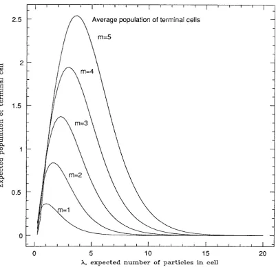
proportional to m. This is because m is the maximum number of bodies that can reside in a terminal cell. As m increases, we expect proportionally more bodies in terminal cells. Furthermore, the value of A, which gives rise to the maximum expected population is also approximately equal to m. The reason is that for significantly higher AI" cells are likely not to be terminal, while for significantly smaller

A"

cells are likely to have low populations, or not to have parents which are internal cells. Figure 2.6 shows the same data as Figure 2.5, but with the axes rescaled to reflect the fact that the heights and widths of the curves in Figure 2.5 are approximately proportional to m.

From Figure 2.6, we see that the expected number of terminal bodies in a cell peaks when AI' is slightly less than m. Furthermore, even for "resonant" values of AI" close to the peak, the expected population of V, is slightly less than about

m/2. Thus we conclude that in a BH tree with a maximum of m bodies per node, we can expect, on average, slightly fewer than m/2 bodies in the terminal nodes. This should not be a surprising result. Consider the fact that the probability that a given node, not necessarily terminal, with AI' ~ m has m bodies is not too much different from the probability that it has m+ 1. In the latter case, it will likely give rise to eight smaller terminal cells, with an average population of only (m

+

1)/8. Thus, almost-empty terminal cells are about as likely as almost-full terminal cells, and it isn't surprising that the average population of terminal cells is near to m/2.

2.7. Average depth of bodies.

Now we can ask for the expected population of all cells with depth equal to d. Clearly, this is just a sum over all appropriate, of Eqn. 2.26,

<

Pop(depth

=

d)

>=

L

Npl'(DN-l,m-l(Ph) - DN-l,m-l(PI')).

I'E Ld

Equation 2.30 may be simplified by noting that

Pa =

L

PI"

,3I(,)=a

(2.30)

(55)

::::

Q)

C)

2.5

2

1.5

0.5

o

Average population of terminal cells

5 10 15 20

A, expected nUInber of particles in cell

(56)

0.6 Scaled expected population vs. A

E

...

1\ 0.4

~ .~

....

ttl

'"5 p.

0

p..

v

0.2

2 3 4

AI

rn

Figure 2.6. The expected value of the number of bodies in a cell with N P, = .A" with both the ordinate and abcissa scaled by m.

(57)

i.e., for a given cell, the sum of the probabilites of its children is equal to its own probability. Thus,

<

Pop(depth

=

d)

>

=

N (

L

P,DN-l,m-l(P,) -

L

P,DN-l,m-l(p,))

,ECd-l ,ECd

= N (FN-1,m-l(d -

1) -

FN-l,m-l(d)) ,

(2.32) where we define

FN,m(d) =

L

p,DN,m(P,). (2.33)

,ECd

We can check our calculation by computing the sum of the expected popula-tion, over all values of d,

00

<

Total population> =

L

<

Pop(depth = d)

>

d=O

~

N

(t,

(FN-l,m-l(d -

1) -

FN-l,m-l(d)))

= N

J~oo

(t

(FN-l,m-l(d - 1) - FN-l,m-l(d)))

d=l

= N Dlim

(FN-1,m-l(O) -

FN-l,m-l(D))

-+00

= N

(1 -

D-+oo

lim FN-1,m-l(D))

=N.

(2.34) The last identity follows from the fact that

(2.35)

by the same argument as led to Eqn. 2.13.

(58)

The average depth of a body in a BH tree may also be obtained from Eqn. 2.31,

1 00

Davg

=

N

~

d

<

Pop(depth

=

d)

>

d=O

D

=

J~oo ~

d(FN-l,m-l(d - 1) - FN-l,m-l(d)))

d=l

D-l

= Dlim

(~FN-l,m-l(d)

- DFN-1,m-l(D))

-+00

d=O

00

=

~

FN-l,m-l(d)

d=O

=

~P,DN-l,m-l(P').

,

(2.36)

The value of FN,m( d) depends on the details of the probability distribution,

p.

We cannot make further progress analyzing the average depth of the BH tree, or the average number of cells it contains, unless we make assumptions about

p.

2.8. Uniforln distribution, i.e.,

p(x)

=

const.

If the distribution of bodies, p( x), is constant, we can explicitly evaluate FN,m( d)

and GN,m(d) and then numerically evaluate C avg and Davg. The results are in-teresting in their own right, as approximately uniform distributions of bodies are used to describe the early universe in cosmological simulations. More importantly, we can extrapolate the results for a uniform distribution to situations with a non-uniform distribution, but a sufficiently large value of N.

We now consider the situation in which

p

is a uniform distribution, i.e., a body is equally likely to appear anywhere in the volume,

Vo.

Since

p(

x)

is a probability density, we have

1

p(x)

=

V

o

'

P

,-

- S-d(,),)

,

(2.37)

(59)

and there are exactly 8d _{cells with depth d. Equation 2.11 becomes}

and Eqn. 2.33 becomes

Now we use Eqns. 2.10 and 2.36 and obtain

and

00

Cavg =

I::

8d _{D N ,m(8-}d) d=o

00

Davg =

I::

DN_1,m_l(S-d).

d=O

(2.39)

(2.40)

(2.41)

(2.42)

We can verify that they are well defined if we make use of the limit, Eqn. 2.8. In fact, Eqn. 2.8 tells us that the sums converge very rapidly and can eaily be evaluated numerically given values Nand m.

Figure 2.7 shows

C

avg computed according to Eqns. 2.41 and 2.10. Based on

the figure one is tempted to conjecture that

NC

m

C

avg

<

-m for all N. (2.43)

A plot of mC;;vg is shown in Figure 2.8, in which the abscissa is remarkably constant

over a large range in N.