Volume 2008, Article ID 213293,14pages doi:10.1155/2008/213293
Research Article
Quad-Quaternion MUSIC for DOA Estimation
Using Electromagnetic Vector Sensors
Xiaofeng Gong, Zhiwen Liu, and Yougen Xu
Department of Electronic Engineering, Beijing Institute of Technology, Beijing 100081, China
Correspondence should be addressed to Yougen Xu,[email protected]
Received 24 April 2008; Revised 22 October 2008; Accepted 22 December 2008
Recommended by Jacques Verly
A new quad-quaternion model is herein established for an electromagnetic vector-sensor array, under which a multidimensional algebra-based direction-of-arrival (DOA) estimation algorithm, termed as quad-quaternion MUSIC (QQ-MUSIC), is proposed. This method provides DOA estimation (decoupled from polarization) by exploiting the orthogonality of the newly defined “quaternion” signal and noise subspaces. Due to the stronger constraints that quaternion orthogonality imposes on quad-quaternion vectors, QQ-MUSIC is shown to offer high robustness to model errors, and thus is very competent in practice. Simulation results have validated the proposed method.
Copyright © 2008 Xiaofeng Gong et al. This is an open access article distributed under the Creative Commons Attribution License, which permits unrestricted use, distribution, and reproduction in any medium, provided the original work is properly cited.
1. INTRODUCTION
A “complete” electromagnetic (EM) vector sensor com-prises six collocated and orthogonally oriented EM sensors (e.g., short dipole and small loop), and provides complete electric and magnetic field measurements induced by an EM incidence [1–3]. An “incomplete” EM vector sensor with one or more components removed is also of high interest in some practical applications [4, 5]. Numerous algorithms for direction-of-arrival (DOA) estimation using one or more EM vector sensors have been proposed. For example, vector sensor-based maximum likelihood strategy was addressed in [6–9], multiple signal classifi-cation (MUSIC [10]) was extended for both incomplete and complete EM vector-sensor arrays in [11–16], sub-space fitting technique was reconsidered for incomplete EM vector sensors in [17, 18], and estimation of signal parameters via rotational invariance techniques (ESPRIT [19]) was revised for EM vector sensor(s) in [20–26]. The identifiability issue of EM vector sensor-based DOA estimation has been discussed in [27–29]. Some other related work can be found in [30–34]. In all the con-tributions mentioned above, complex-valued vectors are used to represent the output of each EM vector sensor in the array, and the collection of an EM vector-sensor array is arranged via concatenation of these vectors into a
“long vector.” Consequently, the corresponding algorithms somehow destroy the vector nature of incident signals carrying multidimensional information in space, time, and polarization.
(8D) algebras, respectively, while a full characterization of the sensor output for complete six-component EM vector sensors requires an algebra with dimensions equal to 12 or more.
Unfortunately, not all algebras having 12 or more dimensions are associative division algebras. For example, sedenions, as a well-known 16D algebra, are neither an associative algebra nor a division algebra [39], and thus are not suitable for the modeling and analysis of vector sensors. In this paper, we use a specific 16D algebra— quad-quaternions algebra [40–42] to model the output of six-component EM vector sensor(s) [3]. This 16D quad-quaternion algebra can be proved to be an associative division algebra, and thus is well adapted to the mod-eling and analysis of complete EM vector sensors. More precisely, We redefine the array manifold, signal subspace, and noise subspace from a quad-quaternion perspective, and propose a quad-quaternion-based MUSIC variant (QQ-MUSIC) for DOA estimation by recognizing and exploit-ing the quaternion orthogonality between the quad-quaternion signal and noise subspaces. QQ-MUSIC here is shown to be more attractive in the presence of two typical model errors, that is, sensor position error and sensor orientation error, which are often encountered in practice.
The rest of the paper is organized as follows. InSection 2, we present introductions on quaternions and quad-quaternion matrices. In Section 3, the quad-quaternion-based MUSIC algorithm is presented. InSection 4, we com-pare the proposed algorithm with some existing methods by simulations. Finally, we conclude the paper inSection 5.
Since this paper concerns several different hypercomplex values, we here summarize the symbols of values that will appear in subsequent sections inTable 1.
2. QUAD-QUATERNIONS AND QUAD-QUATERNION
MATRICES
In this section, we introduce the algebra of quad-quater-nions, and represent some results related to quad-quaternion matrices. The algebras of quaternions and biquaternions are introduced in detail in [35–38] and thus are not addressed here.
2.1. Quad-quaternions and quad-quaternion matrices Quad-quaternion algebras are a class of 16D algebras [40], which were first considered by Albert since the 1930s [41]. (The quad-quaternion algebras mentioned in this paper are termed as thegeneralizedbiquaternion algebras in [40–42]). The quad-quaternion algebra is defined as follows.
Definition 1 (see [42]). Denote H(an,bn) the quaternion
algebra over bases {1,in,jn,kn}, where i2n = an, j2n = bn, injn = −jnin = kn, and an,bn are nonzero real numbers, n=1, 2, then a quad-quaternion algebra over real numbers is the tensor product [40] ofH(a1,b1)andH(a2,b2), denoted by H(a1,b1)H(a2 ,b2 )=H(a1,b1)⊗H(a2,b2).
By definition, we can see that any element p ∈
H(a1,b1)H(a2 ,b2 )can be expressed as
p=p00+I p01+J p02+K p03
+ip10+I p11+J p12+K p13
+jp20+I p21+J p22+K p23
+kp30+I p31+J p32+K p33,
(1)
where
i2=a1, j2=b1, k2= −a1b1,
I2=a2, J2=b2, K2= −a2b2,
i j= −ji=k, IJ= −JI=K,
ki= −ik=j·−a1, KI= −IK=J·−a2,
jk= −k j=i·−b1, JK= −KJ=I·−b2,
lL=Ll,
(2)
wherel=i,j,kandL=I,J,K.
Denote the classical Hamilton quaternions byH [43], and consider the following particular casea1 =b1 = a2 =
b2 = −1, so that H(a1,b1) = H(a2,b2) = H. Then, with an appropriate choice of norm, the tensor product of H and H, denoted by HH = H⊗H, can be proved to be
a division algebra according to [42, Theorem 4.3], so that zero divisors do not exist (note that the quad-quaternions herein mentioned are labeled as thegeneralized biquaternions
in [42], which are different from the classical biquaternions). Since the algebra of quad-quaternions is always an associative algebra [41], thenHH = H⊗His an associative division
algebra.
Furthermore, from (1) we can see that p ∈ HH can be
interpreted as a quaternion with quaternionic coefficients. In addition, if pmn=0 for allm,n=0, 1, 2, 3,pis called a zero quad-quaternion, denoted by p =0. If p00 =1, and all the other coefficients are zero, thenpis called an identity quad-quaternion, denoted by p=1. In addition, p00is called the scalar part ofp, denoted byS(p), while the vector part ofpis given byV(p)=p−S(p).
Besides the expression in (1), a quad-quaternionp∈HH
can as well be expressed as
p=p0+I p1+J p2+K p3=b0+Ib1, (3)
wherepn=p0n+ip1n+j p2n+k p3n∈H,n=0, 1, 2, 3;bm= pm+J pm+2∈HC(J),m=0, 1. In particular,p=b0+Ib1can be considered as a quad-quaternion version of the Cayley-Dickson expression for quaternions and biquaternions in [36, 37]. The definitions of addition and multiplication extend naturally from the case of biquaternion matrices, and thus are not addressed here.
From the geometric perspective, a quad-quaternionp=
Table1: Symbols of algebraic values.
R Real numbers
C(L) Complex numbers with bases{1,L}, whereL=i,j,k,I,J,K. In particular,C(i)is denoted byC.
H(a,b)
Quaternions with bases{1,i,j,k}such thati2=a, j2=bandi j= −ji=k, whereaandbare nonzero real numbers. In particular,H=H(−1,−1)corresponds to the classical Hamilton quaternions
H(1),H(2) H(1)denotes Hamilton’s quaternions with bases{1,i,j,k};H(2)denotes the Hamilton quaternions with bases{1,I,J,K}. In particular, we denoteH(1)byH.
HC(L)
Biquaternions with bases{1,i,j,k,L,Li,L j,Lk},L=I,J,K, such thati2= −1, j2= −1, i j= −ji=kandlL=Ll, where l=i,j,k. In particular, we denoteHC(I)byHC.
HH Quad-quaternions with bases{1,i,j,k,I,Ii,I j,Ik,J,Ji,J j,Jk,K,Ki,K j,Kk}such thati
2=j2=I2=J2= −1, i j= −ji=k,IJ= −JI=K, andlL=Ll, wherel=i,j,kandL=I,J,K.
pare not real values, but four individual quaternions which can be considered as four subpoints in a 4D hypospace spanned by 1,I,J,K. Therefore, quite similar to quaternion rotations [38], we can interpret quad-quaternion multiplica-tions as a more complex 16D “quad-quaternion rotamultiplica-tions” which involve both 4D rotations(quaternion multiplica-tions) and combination of 4D points (quaternion addimultiplica-tions) in spaces spanned by 1,i,j,kand 1,I,J,K.
Definition 2. A quad-quaternion matrixQ∈(HH)M×N is a
matrix withMrows andNcolumns of which each element is a quad-quaternion qm,n ∈ HH,m = 1, 2,. . .,M, n =
1, 2,. . .,N. In particular, anNdimensional quad-quaternion column (row) vector can be considered as an N×1 (1×
N) quad-quaternion matrix. In this paper, quad-quaternion vectors are specifically referred to as column vectors. Similar to the case of quad-quaternion scalars, a quad-quaternion matrixQ∈(HH)M×N can be expressed as follows:
Q=Q00+IQ01+JQ02+KQ03
+iQ10+IQ11+JQ12+KQ13
+jQ20+IQ21+JQ22+KQ23
+kQ30+IQ31+JQ32+KQ33
=Q0+IQ1+JQ2+KQ3=B0+IB1,
(4)
where Qn1n2 ∈ R
M×N, n1,n2 = 0, 1, 2, 3, Q
n ∈ HM×N,
n = 0, 1, 2, 3, and B0,B1 ∈ (HC(J))M×N. Similar to quad-quaternion scalars, the scalar and vector parts ofQare given byS(Q)=Q00andV(Q)=Q−S(Q), respectively.
In the following discussion, we mainly focus on results related to quad-quaternion matrices and vectors. The results related to scalars can be directly obtained by considering a quad-quaternion scalar as a 1×1 quad-quaternion “matrix.”
2.2. Previous relevant results
In this section, we present some results that are directly generalized from quaternion or biquaternion results. All the lemmas in this section can be proved similarly to their quaternion and biquaternion counterparts in [35–37], and thus are not included in this paper.
K
I J 1
k
i
j 1 K
I J
1
K
I J
1 K
I J
1
p3
p3 p0
p2
p2
p1 p1
p=p0+ip1+j p2+k p3
Figure1: The geometric illustration of quad-quaternions.
Definition 3 ([37, Definition 2]). There exist four different conjugations for quad-quaternion matrices as follows.
(i)C-conjugationQC:QC=B0−IB1;
(ii)H1-conjugationQ:Q=Q∗0 +IQ∗1 +JQ∗2 +KQ∗3; (iii)H2-conjugationQ∗:Q∗=Q0−IQ1−JQ2−KQ3; (iv) Total-conjugationQ:Q=Q∗0 −IQ1∗−JQ∗2 −KQ∗3,
where Q∗n denotes the quaternion conjugation of Qn,n = 0, 1, 2, 3, as given in [36].
Definition 4(from [37]). The transpose ofQ=Q0+IQ1+ JQ2 +KQ3 ∈ (HH)M×N, denoted by QT ∈ (HH)N×M, is
defined asQTQT
0+IQT1+JQ2T+KQT3, whereQTndenotes the quaternion transpose ofQn,n=0, 1, 2, 3. Then we have the following four different conjugated transposes.
(i)C-conjugated transposeQ:Q=(QC)T =(QT)C; (ii)H1-conjugated transposeQH1:QH1=(Q)T=(QT); (iii)H2-conjugated transposeQH2:QH2=(Q∗)T=(QT)∗;
(iv) Total-conjugated transposeQH:QH=(Q)T=QT.
Definition 5 ([37, Definition 3]). The norm of a quad-quaternion p = p0+I p1+J p2 +K p3, denoted by|p|, is given by
By definition, we can see that the following equation holds:
S(pp)=Sp∗0−I p∗1−J p∗2−K p∗3
p0+I p1+J p2+K p3
=Sp∗0p0+p∗1p1+p2∗p2+p∗3p3
+Ip∗0p1+p∗3p2−p∗1p0−p∗2p3
+Jp0∗p2+p∗1p3−p∗2p0−p3∗p1
+Kp∗0p3+p∗2p1−p∗3p0−p∗1p2
=p0∗p0+p∗1p1+p∗2p2+p∗3p3
= |p|2.
(6)
It is important to note that |pq|= |/ p||q|, so that quad-quaternions do not form a normed algebra. We can further define the norm of a quad-quaternion vectorq ∈(HH)N×1
by
qSqHq. (7)
Definition 6 (see (15) from [37]). Two quad-quaternion vectorsa,b∈(HH)N×1are said to be orthogonal if
aHb=0. (8)
Definition 7(see (17) from [37]). The adjoint matrix (χQ ∈
(HC(J))2M×2N) of a quad-quaternion matrixQ∈(HH)M×N = B0+IB1(whereB0,B1∈(HC(J))M×N) is given by
χQ
B0 B∗1
−B1 B∗0
. (9)
Let furtherΨM [IM,−I·IM]∈(C(I))M×2M, whereIM is the identity matrix of sizeM×M, then
Q=1
2ΨMχQΨ H
N, (10)
where
ΨMΨHM=2IM, χQΨ
H
NΨN =ΨHMΨMχQ.
(11)
Lemma 1(from [35]). Consider two quad-quaternion matri-cesA∈(HH)M×N andB∈(HH)N×L, and denote the adjoint
matrices ofA,B, andABbyχA,χB, andχAB, respectively, then
χAB=χA·χB. (12)
Lemma 2([37, Lemma 1]). IfPH =P, thenP∈ (H
H)N×N
is Hermitian. Then we note that the adjoint matrix of a Hermitian quad-quaternion matrix is also Hermitian.
Definition 8(from [37]). IfQu=uλ, whereu∈(HH)N×1,
λ∈C, andQ∈(HH)N×N, thenλanduare, respectively, the
right eigenvalue and the associated right eigenvector ofQ.
Lemma 3([37, Lemma 2]). Denote the adjoint matrix ofQ∈
(HH)N×N byχQ, ifλ ∈Candub ∈(HC(J))2N×1are the right
eigenvalue and the associated right eigenvector ofχQ, thenλ
andu=ΨNubare the right eigenvalue and the associated right eigenvector ofQ.
Corollary 1 (from [37]). The eigenvalues of a Hermitian quad-quaternion matrix are real values. Consider a Hermitian quad-quaternion matrixQ∈(HH)N×N whose adjoint matrix
χQ can be eigendecomposed as χQ = UbDUHb, whereUb ∈ (HC)2N×4N, andD∈R(4N×4N)is a real diagonal matrix. The
eigendecomposition ofQis then given by
Q=UDUH= 4N
n=1
λnunuHn, (13)
whereU=(1/√2)ΨNUb ∈(HH)N×4N,λnis thenth element of the diagonal ofD,unis thenth column vector ofU.
Lemma 4. The eigenvectors corresponding to different eigen-values of a Hermitian quad-quaternion matrix are orthogonal.
2.3. New definitions and lemmas for quad-quaternioins
In this section, we introduce some new results related to quad-quaternions. For an easier reading of this section, all the results are given directly, while some of their proofs are summarized in theappendixfor the reference of interested readers.
Definition 9. LetΛ = {1,i,j,k,I,Ii,I j,Ik,J,Ji,J j,Jk,K,Ki, K j,Kk}andΓ⊆Λ, then theΓ-match of a quad-quaternion matrix Q ∈ (HH)M×N, denoted byS(Q | Γ), is obtained
by keeping the coefficients of the units inΓunchanged, and setting all the other coefficients to zero. TheΓ-complement ofQis defined asV(Q|Γ)Q−S(Q|Γ).
By definition, we know that the match and complement operations are used to select some desired parts of quad-quaternions. For example, ifΓ= {1,i,K}, thenS(Q |Γ)= Q00+iQ10+KQ03, whereQ00,Q10,Q03are given in (4). Also it can be proved thatV(Q|Γ⊥)=S(Q|Γ), whereΓ⊥denotes the complement ofΓ. Particularly, ifΓ= {1},S(Q|Γ) and V(Q |Γ) are equal to the scalar part and the vector part of Q, respectively.
Definition 10. LetΛ= {1,i,j,k,I,Ii,I j,Ik,J,Ji,J j,Jk,K,Ki, K j,Kk}, and Γ ⊆ Λ, then the Γ-conjugation of a quad-quaternion matrixQ = S(Q | Γ) +V(Q | Γ) ∈(HH)M×N
is denoted by conj(Q|Γ), and defined as
conj(Q|Γ)S(Q|Γ)−V(Q|Γ). (14)
It should be noted that the four conjugations given in Definition 3 are actually four special examples of the Γ -conjugation corresponding to different selections of Γ. For example, the H1-conjugation corresponds to Γ = {1,I,J,K}, whereas the total-conjugation corresponds toΓ= {i,j,k,I,J,K}⊥.
Lemma 5. Given two setsΓ1,Γ2⊆Λ, we have
conjconjQ|Γ1
|Γ2
=conjQ|Γ1∩Γ2
∪Γ1∪Γ2 ⊥
whereΓ1∩Γ2andΓ1∪Γ2denote the intersection and union of
Γ1andΓ2, respectively.
Definition 11. LetΛ= {1,i,j,k,I,Ii,I j,Ik,J,Ji,J j,Jk,K,Ki, K j,Kk} and Γ ⊆ Λ, the Γ-conjugated transpose of Q is given by conj(Q|Γ)T. It is easy to prove that conj(Q|Γ)T =
conj(QT | Γ). Also, when Γ = Λ, QT = conj(Q|Γ)T . Similar to theΓ-conjugation, the four different conjugated transposes given inDefinition 4are four different examples corresponding to four different selections ofΓ.
Definition 12. Quad-quaternion vectors v1,v2,. . .,vN ∈ (HH)M×1are said to be right (left) linear dependent if there
are scalarsμ1,μ2,. . .,μN ∈HHnot all zero, such thatv1μ1+
v2μ2+· · ·+vNμN = oM×1 (μ1v1+μ2v2+· · ·+μNvN =
oM×1). Moreover, if v1μ1 + v2μ2 + · · · + vNμN = oM×1 (μ1v1 +μ2v2 +· · · +μNvN = oM×1) is true if and only if μ1,μ2,. . .,μN are all zero, vectors v1,v2,. . .,vN are said to be right (left) linearly independent. Here, oN×1 is an N ×1 zero vector. Obviously, since v1μ1=/μ1v1 in most cases, the concept of right linear dependent (independent) is different from that of left linear dependent (indepen-dent).
Definition 13. Given a set of quad-quaternion vectors v1,v2,. . .,vN ∈ (HH)M×1, if v1,v2,. . .,vR (R < N), are right (left) linearly independent and there exists an arbitrary vectorvR+1 ∈ (HH)M×1 such thatv1,v2,. . .,vR+1 are right (left) linearly dependent, then v1,v2,. . .,vR form a maximal right (left) linearly independent set. Further-more, we define the right (left) rank of {v1,v2,. . .,vN} as rankR({v1,v2,. . .,vR}) R (rankL({v1,v2,. . .,vR}) R).
Definition 14. Given a quad-quaternion matrix P = [p1, p2,. . .,pN], where pn is the nth column of P, n = 1, 2,. . .,N. Then the right (left) rank of P is defined as rankR(P) rankR({p1,p2,. . .,pN}) (rankL(P) rankL({p1,p2,. . .,pN})). In addition, we have the following lemma.
Lemma 6. Denote the adjoint matrix ofP∈(HH)N×N byχP, then
rankR(P)= 1 2rankR
χP
rankL(P)= 1 2rankL
χP
.
(16)
In the following discussion, we only consider the right rank, and we denoterank(P)=rankR(P).
Lemma 7. Denote the eigenvalue decomposition of a Hermi-tian quad-quaternion matrixQbyQ=UDUH, then we have
rank(Q)=1
4rank(D). (17)
Definition 15. Given a set of orthogonal quad-quaternion vectors v1,v2,. . .,vN, we can define the vector space R
spanned by v1,v2,. . .,vN as R
v | v = v1μ1 + v2μ2 + · · · + vNμN
, where μ1,μ2,. . .,μN are arbitrary quad-quaternion scalars. R can also be denoted as R =
span(v1,v2,. . .,vN).
Lemma 8. Ifv1,v2,. . .,vN areNeigenvectors of a Hermitian quad-quaternion matrix, then v1μ1,v2μ2,. . .,vNμN are also a set of eigenvectors of this Hermitian quad-quaternion matrix, where μ1,μ2,. . .,μN are nonzero quad-quaternions. Then, we have span(v1,v2,. . .,vN) = span(v1μ1,v2μ2,. . .,
vNμN).
This lemma indicates that the indetermination of eigen-vectors of a Hermitian quad-quaternion matrix does not impact their span. From the geometric perspective, when the eigenvector multiplies a nonzero scalar from the right side, all the elements of this eigenvector are rotated in the 16D quad-quaternion space (as shown in Figure 1) with the same quad-quaternion manner, and the proportional relationship between different elements does not change. Therefore, the intrinsic “structure” of this eigenvector is independent of the above-mentioned eigenvector indetermi-nation.
3. QUAD-QUATERNION MUSIC
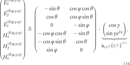
3.1. Quad-quaternion model for EM vector sensors Let (θ,ϕ) and (γ,η) be the azimuth-elevation 2D DOA (see Figure 2) and polarization of an EM signal, respectively, where 0< θ≤2π, 0≤ϕ≤π, and 0≤γ≤π/2,−π≤η≤π. The output of an EM vector sensor then can be capsulated into the following quad-quaternion scalar:
p(θ,ϕ,γ,η)=iE(θ,ϕ,γ,η)
x +IHx(θ,ϕ,γ,η)+jE(yθ,ϕ,γ,η)+IHy(θ,ϕ,γ,η)
+kEz(θ,ϕ,γ,η)+IHz(θ,ϕ,γ,η)
,
(18)
where Ex(θ,ϕ,γ,η), Ey(θ,ϕ,γ,η), Ez(θ,ϕ,γ,η) ∈ C(J), and Hx(θ,ϕ,γ,η), Hy(θ,ϕ,γ,η),Hz(θ,ϕ,γ,η) ∈ C(J) are the three components of the electric vector and the magnetic vector, respectively, which are defined as [2]
⎛ ⎜ ⎜ ⎜ ⎜ ⎜ ⎜ ⎜ ⎜ ⎜ ⎜ ⎜ ⎜ ⎜ ⎜ ⎜ ⎝
E(xθ,ϕ,γ,η)
E(yθ,ϕ,γ,η)
E(zθ,ϕ,γ,η)
Hx(θ,ϕ,γ,η)
Hy(θ,ϕ,γ,η)
Hz(θ,ϕ,γ,η)
⎞ ⎟ ⎟ ⎟ ⎟ ⎟ ⎟ ⎟ ⎟ ⎟ ⎟ ⎟ ⎟ ⎟ ⎟ ⎟ ⎠
⎛ ⎜ ⎜ ⎜ ⎜ ⎜ ⎜ ⎜ ⎜ ⎜ ⎜ ⎝
−sinθ cosϕcosθ
cosθ cosϕsinθ 0 −sinϕ
−cosϕcosθ −sinθ
−cosϕsinθ cosθ
sinϕ 0 ⎞ ⎟ ⎟ ⎟ ⎟ ⎟ ⎟ ⎟ ⎟ ⎟ ⎟ ⎠
·
cosγ sinγeJη
hγ,η∈
C(J)2×1 .
(19)
pθ,ϕ,γ,η = ⎧ ⎪ ⎪ ⎪ ⎪ ⎪ ⎪ ⎪ ⎪ ⎨ ⎪ ⎪ ⎪ ⎪ ⎪ ⎪ ⎪ ⎪ ⎩ Θ(1) θ,ϕ∈
C(I)1×2
−sinθ−I·cosϕcosθ cosϕcosθ−I·sinθ
T
·i+
Θ(2)
θ,ϕ∈
C(I)1×2
cosθ−I·cosϕsinθ cosϕsinϕ+I·cosϕ
T
·j+ Θ(3)
θ,ϕ∈
C(I)1×2
I·sinϕ
−sinϕ T
·k
Θθ,ϕ∈H1C×2
⎫ ⎪ ⎪ ⎪ ⎪ ⎪ ⎪ ⎪ ⎪ ⎬ ⎪ ⎪ ⎪ ⎪ ⎪ ⎪ ⎪ ⎪ ⎭
·hγ,η. (20)
For an array of N EM vector sensors, the spatial steering vectordθ,ϕis given by
dθ,ϕ =
eJ·2π(kT
1eθ,ϕ/λ),. . .,eJ·2π(kTNeθ,ϕ/λ)T, (21)
whereknis the position vector of thenth EM vector sensor,
eθ,ϕis the propagation vector corresponding to (θ,ϕ),λis the wavelength of incident signals. The steering vector of such an N-element EM vector-sensor array then can be expressed as
aθ,ϕ,γ,η= pθ,ϕ,γ,ηdθ,ϕ =
Θθ,ϕ⊗dθ,ϕ
hγ,η
=Θ(1)
θ,ϕ⊗dθ,ϕ
hγ,η
a(1)θ,ϕ,γ,η
·i+Θ(2)θ,ϕ⊗dθ,ϕ
hγ,η
a(2)θ,ϕ,γ,η
·j
+Θ(3)θ,ϕ⊗dθ,ϕ
hγ,η
a(3)θ,ϕ,γ,η
·k,
(22)
where “⊗” denotes the Kronecker product.
In the presence ofM narrowband, far-field, and com-pletely polarized signals, the quad-quaternion model of an N-element EM vector-sensor array has the following form:
x(t)=
M
m=1
amsm(t) +n(t)
=
M
m=1
Θm⊗dm
·hm
·sm(t) +n(t),
(23)
wheresm(t)∈C(J)is the complex envelop of themth signal, andn(t) is the additive noise term, anddm =dθm,ϕm,pm =
pθm,ϕm,γm,ηm,Θm = Θθm,ϕm,hm = hγm,ηm. It is assumed here
that (1) all the incident signals are uncorrelated; (2) the noise is spatially white and uncorrelated with the signals; (3) steering vectors corresponding to different selections of (θ,ϕ,γ,η) are right linearly independent.
3.2. Algorithm details
We first define the quad-quaternion array manifoldΦas the continuum of steering vectoraθ,ϕ,γ,ηin the angular parameter space of interestI1and the polarization parameter space of interestI2. That is,
Φ aθ,ϕ,γ,η, (θ,ϕ)∈I1, (γ,η)∈I2
. (24)
Moreover, the signal subspace and noise subspace in quad-quaternion case are defined as follows:
Rs=span
a1,. . .,aM
,
Rn=R⊥s .
(25)
Define the covariance matrix with quad-quaternion entries as
Rx=E
xtl
xHt
l
, (26)
where “E” denotes expectation. From (23),
Rx= M
m=1
σ2
mamaHm+Rn, (27)
whereσ2
m=E[sm(t)s∗m(t)] andRn=E[n(t)nH(t)]=σn2IN. It can be easily proven according toDefinition 14 that the rank of A = [a1,a2,. . .,aM] isM, then in the absence of noise, the rank ofRx = diag([σ12,σ22,. . .,σM2])AAH isM, and the column vectors ofRxspan the signal subspaceRs. In the presence of noise, we apply an M-rank approximation of Rx to estimate the bases of signal subspace. According toLemma 7, we know that the bestM-rank approximation ofRx has 4M eigenvalues, thus we can use the eigenvectors
v1,. . .,v4Massociated with the largest 4Meigenvalues as the bases of signal subspaces. DenoteEs=[v1,. . .,v4M] andEn= [v4M,. . .,v4N], then Rs = span(Es) and Rn = span(En). Further, definePn =EnEHn ∈HHN×N, we havePnam = 0, then
θm,ϕm
=arg min
θ,ϕ,γ,η
!!Pnaθ,ϕ,γ,η!!". (28)
In the presence of finite data length,Rxcan be estimated as follows:
# Rx= 1
L L
l=1
x(tl)xH(tl). (29)
Accordingly,EnandPncan be estimated by eigendecompos-ingR#x.
3.3. Decoupling of angular and polarization parameters
According to (28), a 4D search is required for DOA estimation, which might be computationally prohibitive. We next discuss how to decouple polarization from DOA estimation for the purpose of reducing the computational burden. Firstly, we prove the following lemma.
Lemma 9. Given h ∈ (C(L))M×1,L ∈ {i,j,k,I,J,K}and a
Hermitian matrixF ∈(HH)M×M, thenS(hHFh)= hHS(F|
{1,L})h. Here,S(hHFh)and S(F | {1,L})denote the scalar part of hHFhand the{1,L}-match ofF, respectively.
Proof. Without loss of generality, we assumeL = J. Hence, h∈(C(J))M×1. Let furtherF=(F
00+IF01) +i(F10+IF11) + j(F20+F21) +k(F30+F31), thenS(F | {1,J}) = F00. Since FH=F, we haveFH
00=F00. Then it is further obtained that
ShHFh=ShHF 00+IF01
+iF10+IF11
+jF20+F21
+kF30+F31
h
=ShHF00h
=hHF00h=hHS
F| {1,J}h. (30)
We use the above-mentioned lemma to discuss the decoupling of angular and polarization parameters. Letu=
Pnaθ,ϕ,γ,η∈H(HN×1), then
!!Pnaθ,ϕ,γ,η!!=
SuHu. (31)
According to (23), and denoteΞθ,ϕ =Pn·Θθ,ϕ⊗dθ,ϕ, then we have the following equation fromLemma 9:
SuHu=ShHγ,ηΞHθ,ϕΞθ,ϕhγ,η
=hHγ,ηS
ΞH
θ,ϕΞθ,ϕ| {1,J}
hγ,η.
(32)
Note further that hH
γ,ηhγ,η = 1 and S(ΞθH,ϕΞθ,ϕ | {1,J}) is a complex-valued Hermitianmatrix, then according to the Rayleigh-Ritz theorem [11], we obtain
min
θ,ϕ,γ,η
!!Pnaθ,ϕ,γ,η!!= min
θ,ϕ,γ,η
hH
γ,ηS
ΞH
θ,ϕΞθ,ϕ| {1,J}
hγ,η
hH
γ,ηhγ,η
=λminSΞHθ,ϕΞθ,ϕ| {1,J}
,
(33)
whereλmin(S(ΞHθ,ϕΞθ,ϕ | {1,J})) denotes the smallest eigen-value ofS(ΞHθ,ϕΞθ,ϕ| {1,J}). Thus, the 4D search problem is reduced to a 2D search.
For clarity, we finally summarize the above split method (termed as QQ-MUSIC) as follows:
Step 1. calculate the sampled covariance matrixR#xaccording to (29);
Step 2. apply the quad-quaternion EVD to R#x, select the 4(N−M) eigenvectors associated to the smallest 4(N−M) eigenvalues, and calculate the noise subspace projectorPn;
z
y
x
θ
ϕ
Figure2: Coordinate system and angle definition.
Step 3. given an arbitrary (θ,ϕ)∈I1, calculateΞθ,ϕ =Pn·
Θθ,ϕ⊗dθ,ϕandS(ΞθH,ϕΞθ,ϕ| {1,J}).
Step 4. then the DOA estimates are obtained by
arg min (θ,ϕ)∈I1
λminFθ,ϕ
. (34)
It is important to note that QQ-MUSIC cannot ful-fill simultaneous estimation of DOA and polarization. The problem of polarization estimation or joint DOA-polarization estimation remains unresolved and is currently under investigation by the authors.
3.4. Computation complexity
In this section, the computational complexity of QQ-MUSIC, BQ-QQ-MUSIC, and long-vector MUSIC is addressed. As addressed in [36,37], the covariance matrix estimation best illustrates the complexity difference of the three algo-rithms, therefore we only consider the computational com-plexity involved in this part. The evaluation of computational complexity includes two aspects: memory requirement and number of real number additions (A), multiplications (M), and divisions (D).
Assume that the array comprisesNcomplete EM vector sensors, and T snapshot vectors are available. The quad-quaternion array outputX∈(HH)N×Tthen is given by
X=X0+IX1=
iX01+jX02+kX03
+IiX11+jX12+kX13
, (35)
where X0,X1 ∈ (HC(J))N×T, and X0n,X1n ∈ (C(J))N×T, n = 1, 2, 3. Then the biquaternion data model (Xb ∈ (HC(J))2N×T) and the long-vector data model (Xlv ∈ (C(J))6N×T) for the same array output are, respectively, written as
Xb=
XT0,XT1
T
, Xlv=
XT01,XT02,XT03,XT11,XT12,X13T T
. (36)
Moreover, the sampled covariance matrices in the three models can be calculated as follows:
# RQ= 1
TXX
H, R#
B= 1 TXbX
H
b, R#LV= 1
TXlvX H
lv,
Table2: Computational effort for covariance estimation.
Memory requirements (complex values) Real multiplications Real additions Real divisions
QQ-MUSIC 8N2 256N2T (256T−16)N2 16N2
(D)
BQ-MUSIC 16N2 256N2T (256T−32)N2 32N2
(D)
LV-MUSIC 36N2 144N2T (144T−72)N2 72N2
(D)
whereR#Q,R#B, R#LVare sampled covariance matrices used in QQ-MUSIC,BQ-MUSIC, and LV-MUSIC, respectively.
From (37), R#Q has N2 entries, each of which is quad-quaternion valued and can be represented by eight complex numbers. Therefore, a memory of at least 8N2 complex numbers is required in the quad-quaternion case. Similarly, for biquaternion and long-vector models, 16N2 and 36N2 complex numbers are required, respectively.
Let us now evaluate the total number of basic arithmetic operations needed for estimation of the covariance matrix. As revealed by (37), every entry of R#Q is obtained by T quad-quaternion multiplications, T − 1 quad-quaternion additions, and a division by a real value. Note that one quad-quaternion multiplication implies 162 real multiplications plus 16×15 real additions, one quad-quaternion addition implies 16 real additions, and the division by a real value equals 16 real divisions. The number of operations needed for one entry is162(M)+ 16×15(A)
T+ 16(T−1)(A)+ 16(D), where subscripts “(M),” “(A),” “(D)” denote real multiplica-tion, real addimultiplica-tion, and real division, respectively. Thus, the total number is{[162
(M)+16×15(A)]T+16(T−1)(A)+16(D)}· N2 = 256N2T(
M) + (256T −16)N(2A)+ 16N(2D). Similarly, the total numbers of arithmetic operations in biquaternion and long-vector models are given by 256N2T(
M)+ (256T− 32)N2
(A) + 32N(2D) and 144N2T(M) + (144T − 72)N(2A) + 72N2
(D), respectively. Table 2 summarizes the covariance matrix computational efforts for all the three algorithms. We can see that QQ-MUSIC largely reduces the memory requirements, mainly due to the more economical formulism of quad-quaternion model. In addition, with regard to basic arithmetic operation number, we can see that QQ-MUSIC requires 16N2 less real divisions and 16N2 more real additions than BQ-MUSIC. Since the computational complexity of divisions is much more than that of additions, QQ-MUSIC slightly outperforms BQ-MUSIC in this aspect. We may also note that LV-MUSIC requires least operations for estimating the covariance matrix, which conflicts our intuition that a more concise model should lead to less computational complexity. This fact can be explained as follows. In QQ-MUSIC, we are using a 16D algebra to model six-component vector sensors, and only twelve imaginary units of quad-quaternions are used in this formulation. Therefore, this insufficient use of quad-quaternions results in more arithmetic operations.
3.5. Orthogonality-measure comparison
As addressed in [37], vector orthogonality in higher dimen-sional algebra imposes stronger constraints on vector com-ponents. In this part, we take a further look into the quad-quaternion-related orthogonality.
Consider two quad-quaternion vectorsx,y ∈(HH)Nx×1
given by
x=x01+Ix11
i+x02+Ix12
j+x03+Ix13
k,
y=y01+Iy11
i+y02+Iy12
j+y03+Iy13
k. (38)
The corresponding biquaternion representation and com-plex representation then can be written as
xbq=
xT01, x11T T
i+xT02, x12T T
j+x03T, xT13 T
,
k∈HC2Nx×1,
ybq=
y01T, y11T T
i+yT02, yT12 T
j+yT03, yT13 T
,
k∈HC2Nx×1,
xc=
xT01, xT11, x02T, xT12, xT03, xT13 T
∈C(J)6Nx×1
,
yc=
yT01, yT11, y02T, yT12, yT03, y13T T
∈C(J)6Nx×1
. (39)
Imposing the orthogonal constraint on quad-quaternion vectors (xHy=0) yields
xH
01y01+xH11y11+xH02y02+xH12y12+xH03y03+xH13y13=0,
xT
01y11−xT11y01+xT02y12−xT12y02+xT03y13−xT13y03=0,
xH
02y03+x12Hy13−xH03y02−x13Hy12=0,
xT
02y13−xT12y03−xT03y12+x13Ty02=0,
xH03y01+x13Hy11−xH01y03−x11Hy13=0,
xT03y11−xT13y01−xT01y13+x11Ty03=0,
xH01y02+x11Hy12−xH02y01−x12Hy11=0,
xT01y12−xT11y02−x02Ty11+x12Ty01=0.
(40)
In contrast, orthogonal constraint on biquaternion vectors (xH
bqybq=0) results in
xH01y01+xH11y11+xH02y02+xH12y12+xH03y03+xH13y13=0,
xH02y03+x12Hy13−xH03y02−x13Hy12=0,
xH03y01+x13Hy11−xH01y03−x11Hy13=0,
xH01y02+x11Hy12−xH02y01−x12Hy11=0.
(41)
Moreover, the orthogonal constraint on complex vectors (xH
c yc=0) leads to
y
x d
d d×$Pe
d×$Pe
Actual sensor position Ideal sensor position
Figure3: An array with sensor position errors.
By comparing (40), (41) and (42), it is obtained that:
xHy=0=⇒xbqHybq=0=⇒xcHyc=0. (43)
Consequently, the quad-quaternion orthogonality can impose stronger constraints than both biquaternion and complex algebra do. This property of quad-quaternions results in a better robustness of QQ-MUSIC to model errors, as to be demonstrated inSection 4.
4. SIMULATION RESULTS
In this section, simulation results are provided to compare the proposed QQ-MUSIC with both biquaternion-based (such as BQ-MUSIC) and complex-based methods (such as LV-MUSIC) for six-component EM vector-sensor arrays. It should be noted that BQ-MUSIC was actually proposed for three-component vector-sensor arrays [37]. Therefore, we here use a 2 ×1 biquaternion vector to represent a six-component vector sensor, and further we concatenate these vectors into a biquaternion long-vector to enable BQ-MUSIC.
We compare the proposed QQ-MUSIC with BQ-MUSIC, LV-MUSIC, and polarimetric smoothing algorithm (PSA-MUSIC [30]), in terms of robustness to model errors and DOA estimation performance under different levels of signal-to-noise ratio (SNR). All the statistics shown here are computed by averaging the results of 200 independent trials. The array used here is an L-shaped array that comprises four and five EM vector sensors along thex-axis andy-axis, respectively (seeFigure 3). The spacing between two adjacent EM vector sensors isd=λ/2. Before representing the results, we introduce the following two model errors.
y
x
z b
a
(a)
y
x
z b
a Norm of the loop
(b)
Figure4: A short dipole or loop with arbitrary orientation.
Sensor-position error
the positions of EM vector sensors are not precisely known. In the simulations, we model such sensor position error by additive uniformly distributed noise, that is,
kn=kn+
Pe·d·
εx,εy, 0
T
, (44)
whereknandknare the actual and ideal position coordinates of the nth EM vector sensor, respectively, εx and εy are uniformly distributed noise terms, and Pe is the power of sensor position error.
Sensor-orientation error
the orientation angles of a dipole and a loop are illustrated in Figure 4. With an orientation angle (α,β), where α ∈
[0, 2π),β∈[0,π/2], the outputs of a dipole and a loop are, respectively, given by
Eα(θ,β,ϕ,γ,η)=[cosαsinβ, sinαsinβ, cosβ]
·Ex(θ,ϕ,γ,η),E(yθ,ϕ,γ,η),Ez(θ,ϕ,γ,η)
T,
Hα(,θβ,ϕ,γ,η)=[cosαsinβ, sinαsinβ, cosβ]
·Hx(θ,ϕ,γ,η),Hy(θ,ϕ,γ,η),Hz(θ,ϕ,γ,η)T,
(45)
the three dipoles of thenth EM vector sensor be (α1,n,β1,n), (α2,n,β2,n), and (α3,n,β3,n), while the orientation angles of the three loops be (α4,n,β4,n), (α5,n,β5,n), and (α6,n,β6,n), then we have
αl,n,βl,n
=αl,βl
+
Pe
εα,l,n,εβ,l,n
,
l=1,. . ., 6; n=1,. . .,N, (46)
where Pe is the power of the sensor orientation error, εα,l,n,εβ,l,nare uniformly distributed noise terms, (α1,β1) = (α4,β4) = (0,π/2), (α2,β2) = (α5,β5) = (π/2,π/2), (α3,β3) = (α6,β6) = (0, 0) are the corresponding nominal orientation angles in the absence of sensor orientation error. Combining (22), (23), (45), and (46), the output of thenth EM vector sensor equals
p(θn,ϕ),γ,η=
% ⎛
⎝cosεβ,1,nsin
εα,1,n−ϕ
−I·sinεβ,4,nsinθ−cos
εα,4,n−ϕ
cosεβ,4,ncosθ
cosεβ,1,ncosθcos
εα,1,n−ϕ
+ sinεβ,1,nsinθ+I·cosεβ,4,nsin
εα,4,n−ϕ
⎞ ⎠
T
·i
+ ⎛
⎝cosεβ,2,ncos
εα,2,n−ϕ
−I·sinεβ,5,nsinθ−sin
εα,5,n−ϕ
cosεβ,5,ncosθ
cosεβ,2,ncosθsin
ϕ−ε1,2,n
+ sinεβ,2,nsinθ+I·cosεβ,5,ncos
εα,5,n−ϕ
⎞ ⎠
T
·j
+ ⎛
⎝sinεβ,3,nsin
εα,3,n−ϕ
+I·cosεβ,6,nsinθ−cos
εα,6,n−ϕ
sinεβ,6,ncosθ
sinεβ,3,ncosθcos
εα,3,n−ϕ
−cosεβ,3,nsinθ+I·sinεβ,6,nsin
εα,6,n−ϕ
⎞ ⎠
T
·k &
·hγ,η.
(47)
Accordingly, the quad-quaternion expressions of the steering vector and the array output can be, respectively, modified as
aθ,ϕ,γ,η =
p(1)θ,ϕ,γ,ηeJ·2π(k
T
1eθ,ϕ/λ),. . .,p(N)
θ,ϕ,γ,ηeJ·2π(k
T
Neθ,ϕ/λ)T,
x(t) =
M
m=1
aθm,ϕm,γm,ηmsm(t) +n(t).
(48)
In the first experiment, we assume that only the sensor position error exists. Three uncorrelated signals are from (θ1,ϕ1) = (8◦, 90◦), (θ2,ϕ2) = (35◦, 90◦), and (θ3,ϕ3) =
(60◦, 90◦) (to exclude the effect of DOA ambiguity on the comparison, we here only consider azimuth angle estima-tion), respectively, with polarizations (γ1,η1) = (45◦, 0◦), (γ2,η2)=(45◦, 90◦), and (γ3,η3)=(45◦, 180◦), respectively. The sensor noise is assumed to be Gaussian white and uncorrelated with the incident signals. The overall root mean square error (RMSE) performance measure used here is defined as follows:
ε= 1
M M
m=1
' ( ( ( )1
N
Ns
n=1
θm−θ#n,m
2
, (49)
whereθ#n,m is the estimate of true azimuth angleθm in the nth trial. It is plotted inFigure 5that the curves of overall RMSE against sensor position error power for QQ-MUSIC, BQ-MUSIC, LV-MUSIC, and PSA-MUSIC wherein the SNR and the number of snapshots are fixed as 30 dB and 1000, respectively. It can be seen that QQ-MUSIC provides the best estimation accuracy in the presence of sensor position error. In the second experiment, we assume that only the sensor orientation error exists. The DOAs and polarizations of the incident signals are the same as the first example. The overall RMSE curves of QQ-MUSIC, BQ-MUSIC, LV-MUSIC, and
Ov
er
all
RMSE
(deg
ree)
0 0.2 0.4 0.6 0.8 1 1.2 1.4
Power of sensor-position error
0 0.01 0.02 0.03 0.04 0.05 0.06 0.07
QQ-MUSIC BQ-MUSIC
LV-MUSIC PSA-MUSIC
Figure 5: RMS estimation errors versus sensor position error power.
Ov
er
all
RMSE
(deg
ree)
0 1 2 3 4 5 6 7
Power of sensor-orientation error
0 1 2 3 4 5 6 7 8 9 10
QQ-MUSIC BQ-MUSIC
LV-MUSIC PSA-MUSIC
Figure 6: RMS estimation errors versus the power of sensor orientation error.
Ov
er
all
RMSE
(deg
ree)
0 0.2 0.4 0.6 0.8 1 1.2
SNR (dB)
−10 −8 −6 −4 −2 0 2 4 6 8 10
QQ-MUSIC BQ-MUSIC
LV-MUSIC PSA-MUSIC
Figure 7: RMS estimation errors versus SNR for an ideal EM vector-sensor array.
We next compare the performance of QQ-MUSIC with BQ-MUSIC, LV-MUSIC, and PSA-MUSIC with respect to SNR. The DOAs and polarizations are the same as the first two examples. The SNR is varied between−10 dB and 10 dB. Three cases are considered (1) in the absence of model error; (2) in the presence of sensor position error only, and the error power is Pe = 0.05; (3) in the presence of sensor orientation error only, with model error power Pe = 5. The results are given in Figures 7–9. From Figure 7, in a model error-free case, QQ-MUSIC and BQ-MUSIC are a bit inferior to LV-MUSIC and PSA-MUSIC. FromFigure 8, we can see that QQ-MUSIC outperforms BQ-MUSIC,
LV-Ov
er
all
RMSE
(deg
ree)
0.5 1 1.5 2 2.5 3 3.5 4 4.5 5
SNR (dB)
−10 −8 −6 −4 −2 0 2 4 6 8 10
QQ-MUSIC BQ-MUSIC
LV-MUSIC PSA-MUSIC
Figure 8: RMS estimation errors versus SNR in the presence of sensor position errors.
Ov
er
all
RMSE
(deg
ree)
0 2 4 6 8 10 12 14
SNR (dB)
−10 −8 −6 −4 −2 0 2 4 6 8 10
QQ-MUSIC BQ-MUSIC
LV-MUSIC PSA-MUSIC
Figure 9: RMS estimation errors versus SNR in the presence of sensor orientation errors.
MUSIC, and PSA-MUSIC at all levels of SNR, in the presence of sensor position errors; fromFigure 9, we see that QQ-MUSIC outperforms LV-MUSIC and PSA-MUSIC in sensor orientation errors, while slightly underperforms PSA-MUSIC because the performance of the latter is independent of sensor orientation errors.
QQ-MUSIC
(dB)
10−4
10−3
10−2
10−1
100
Azimuth angle (degree)
10 20 30 40 50 60 70
Figure10: QQ-MUSIC spectrum in the presence of several close signals; SNR=30 dB, the number of snapshots is 100.
BQ-MUSIC
(dB)
10−4
10−3
10−2
10−1
100
Azimuth angle (degree)
10 20 30 40 50 60 70
Figure11: BQ-MUSIC spectrum in the presence of several close signals; SNR=30 dB, the number of snapshots is 100.
LV
-MUSIC
(dB)
10−4
10−3
10−2
10−1
100
Azimuth angle (degree)
10 20 30 40 50 60 70
Figure12: LV-MUSIC spectrum in the presence of several close signals; SNR=30 dB, the number of snapshots is 100.
angular and polarization domains: (θ1,ϕ1) = (18◦, 90◦), (θ2,ϕ2) = (20◦, 90◦), (θ3,ϕ3) = (40◦, 90◦), (θ4,ϕ4) =
(41◦, 90◦), (θ5,ϕ5) = (65◦, 90◦), and (θ6,ϕ6) = (67◦, 90◦); (γ1,η1) = (γ2,η2) = (γ3,η3) = (γ4,η4) = (γ5,η5) =
(γ6,η6)= (0◦, 0◦) (to exclude the effect of DOA ambiguity on the comparison, we here only consider azimuth angle estimation). In addition, we assume that no model error exists for the above-mentioned array, the SNR is 30 dB, and the number of snapshots is 100. The spectra of QQ-MUSIC, BQ-QQ-MUSIC, and LV-MUSIC are given in Figures 11-12, in which the dotted lines indicate the true azimuth angles. We note that both BQ-MUSIC and LV-MUSIC fail to distinguish the third and the fourth signals, while QQ-MUSIC can successfully distinguish all the six sources with considerable accuracy.
5. CONCLUSIONS
In this paper, we have proposed a new DOA estimator, termed as quad-quaternion MUSIC (QQ-MUSIC), for six-component EM vector-sensor arrays. This new MUSIC vari-ant has employed a newly developed quad-quaternion model that provides a less memory-consuming way to deal with six-component EM vector-sensor outputs. Moreover, with sensor position error or sensor orientation error present, QQ-MUSIC has been shown to be able to offer better DOA estimation accuracy than both biquaternion-MUSIC (BQ-MUSIC) and long-vector MUSIC (LV-(BQ-MUSIC). Thus, QQ-MUSIC may be more attractive than the examined methods in many practical situations, where model errors cannot be ignored.
APPENDIX
PROOFS OF LEMMAS5–8IN SECTION2
Proof of Lemma 5. If we denote conj(Q|Γ3)=conj((conj(Q
| Γ1)) | Γ2), then by definition, Γ3 is a set consisting of the bases whose coefficients are not inversed. Obviously, the coefficients of bases in Γ1 ∩Γ2 are not inversed, and the coefficients of bases in (Γ1∪Γ2)⊥ are inversed twice so that they are also not inversed. Therefore, Γ3 = (Γ1 ∩Γ2)∪ (Γ1∪Γ2)⊥.
Proof ofLemma 6.Without loss of generality, here we only consider the case of right rank. Assume the right rank of P ∈ (HH)M×N isR, then by definition there exists a set of
Rcolumn vectorsq1,q2,. . .,qRofPandRquad-quaternion scalarsλ1,λ2,. . .,λR, such that
q1λ1+q2λ2+· · ·+qRλR=oM×1⇐⇒λ1=λ2=· · ·=λR=0. (A.1)
Moreover, for an arbitrary nonzero column vectorqR+1ofP, there existR+ 1 quad-quaternion scalarsμ1,μ2,. . .,μR,μR+1 not all zero, such that