Earth Planets Space,64, 753–757, 2012
Ionogram inversion for MARSIS topside sounding
Xiuhong Han1,2and Weixing Wan1
1Beijing National Observatory of Space Environment, Institute of Geology and Geophysics, Chinese Academy of Sciences, Beijing 100029, China
2Graduate University of Chinese Academy of Sciences, Beijing 100049, China
(Received October 19, 2011; Revised March 30, 2012; Accepted March 30, 2012; Online published September 18, 2012)
In the present paper, we propose a method of ionogram inversion to retrieve the electron density profile,Ne(h),
of the Martian ionosphere from the topside ionogram, which is measured by the Mars Advanced Radar for Subsurface and Ionosphere Sounding (MARSIS) instrument on board the Mars Express spacecraft. The new inversion technique is developed from Titheridge’s method by replacing the prior polynomials with empirical orthogonal functions (EOFs), which are estimated from the archivedNe(h)observation by the radio occultation
of Mars Global Surveyor (MGS). The EOF-based technique has achieved quick convergence and good stability. It is concluded that the newly developed method is an alternative tool for the analysis of MARSIS ionograms.
Key words:Martian ionosphere, MARSIS ionogram, ionogram inversion.
1.
Introduction
An ionogram is a representation of data from modern and classical ionosondes as a two-dimensional image, display-ing the ionospheric echo intensity versus radio frequency,
f, and time delay (or apparent height) of the radio prop-agation. Through the ionospheric dispersion, the echo ap-parent height, h(f), as a function of radio frequency, is
determined by the unknown height profile, Ne(h), of the
ionospheric electron density. Thus, it is possible to com-pute Ne(h)fromh(f), which is usually digitized directly
from an ionogram. The computation of the electron density profile is usually referred to as an inversion.
Many methods of ionogram inversion have been pro-posed and developed since the ionosonde was put into use in the 1930s. The initial theory of calculating Ne(h)
fromh(f), known as Abel’s integral equation, is given by Whittaker and Watson (1927). Budden (1961) proposed an analytical inversion of Abel’s integral equation which de-scribes the vertical radio wave propagation in an isotropic ionosphere. When the anisotropy is considered, the inver-sion becomes quite complicated, and lamination methods might be used (Jackson, 1969). However, a lamination method needs a completeh(f)trace with high frequency resolution, and cannot include the valleys (such as the E-F valley) in Ne(h), whereas some valley model incorporated
in the polynomial methods may be used to solve the val-ley problem. Therefore, the lamination methods are now rarely used in practice. Titheridge (1961, 1967a, b, 1969, 1975, 1988) proposed a model-fitting method, or polyno-mial analysis in which the curve of true height vs. plasma frequency, h(fp), is represented as a single or
overlap-Copyright cThe Society of Geomagnetism and Earth, Planetary and Space Sci-ences (SGEPSS); The Seismological Society of Japan; The Volcanological Society of Japan; The Geodetic Society of Japan; The Japanese Society for Planetary Sci-ences; TERRAPUB.
doi:10.5047/eps.2012.03.006
ping polynomial(s). Huang and Reinisch (1982) further de-veloped the polynomial analysis by replacing Titheridge’s Taylor polynomials with shifted Chebyshev polynomials, and applied it to the data processing of ISIS topside iono-grams. Reinisch and Huang (1983) further applied this method in the analysis of ground-based Digisonde iono-grams. Recently, researchers have developed the traditional polynomial analysis by replacing the polynomials (Taylor or shifted Chebyshev polynomials) with empirical orthogo-nal functions (EOFs). For example, Dinget al.(2007) have used the EOF series to represent the electron density profile in the ionosphericFlayer at Wuhan, China.
The Mars Advanced Radar for Subsurface and Iono-sphere Sounding (MARSIS) aboard the Mars Express is the first topside sounder designed to characterize the interac-tions of the solar wind with the ionosphere and upper at-mosphere of Mars. The details of the MARSIS instrument and the Mars Express spacecraft have been described by Picardi et al. (2004), Chicarro et al. (2004) and Nielsen (2004). Up to now, MARSIS has recorded a large number of topside ionograms, most of which remain to be inverted or well-inverted. The inversion method frequently used, at present, for these MARSIS ionograms is the lamination method (Nielsenet al., 2006; Morganet al., 2008; Zouet al., 2010). Meanwhile, the analytical inversion of Abel’s in-tegral equation is also used to give the analytical expression of the electron density profiles (Gurnett et al., 2008). In this work, we adopt the EOF series to represent the electron density profile in the Martian topside ionosphere. In the fol-lowing, Section 2 briefly describes the MARSIS ionograms and their scaling. Section 3 discusses the EOF-based inver-sion. In Section 4, our inversion technique is applied to the data of six MARSIS ionograms.
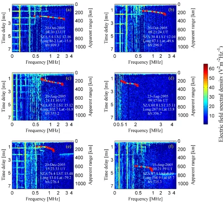
Fig. 1. Ionograms and their scaling. The color-coded echo intensity is plotted as a function of sounding frequency,f, vs. time delay,t, or apparent range,z. The red crosses show the apparent ranges scaled with the process in Section 2.
2.
MARSIS Ionograms and Apparent Range
Scal-ing
Figure 1 displays several topside ionograms obtained by MARSIS at different solar zenith angles (SZAs), latitudes and local true solar time (LST). For a detailed description of the MARSIS ionograms, one can refer to Gurnettet al. (2008) and Morganet al.(2008).
In Figs. 1(a)–(f), the strong vertical lines near the left edge of the ionogram represent harmonics of the local plasma frequency and are caused by the excitation of elec-trostatic oscillations at the local plasma frequency. By measuring the spacing between these harmonics, the lo-cal plasma frequency can be determined and will be used later in our inversion. The technique for measuring the lo-cal plasma frequency is discussed in detail by Duruet al. (2008).
As shown in Figs. 1(a)–(f), in general, the ionospheric echo appears with a time delay that increases with increas-ing frequency and terminates in a well-defined cusp region. The cusp of the echo trace is caused by the rather long time delay that occurs as the sounding frequency is very close
to the peak ionospheric plasma frequency. Hence, the peak plasma frequency of the ionosphere can be determined from the echo cusp.
A semi-automated process, similar to that proposed by Morganet al.(2008), is used to extracth(f)from the iono-spheric echo of the ionogram. The scaled apparent ranges are indicated by the red crosses, as shown in Figs. 1(a)–(f).
3.
Inversion Procedure
In this paper, we develop an inversion procedure by replacing the polynomials (Taylor or shifted Cheby-shev polynomials) with EOFs which are calculated from the archived electron density profiles measured by Mars Global Surveyor (MGS) radio occultation. These archived electron density profiles are available on the website http://nova.stanford.edu/projects/mgs/eds-public.html.
3.1 The archived data and the EOF analysis
X. HAN AND W. WAN: IONOGRAM INVERSION FOR MARSIS TOPSIDE SOUNDING 755
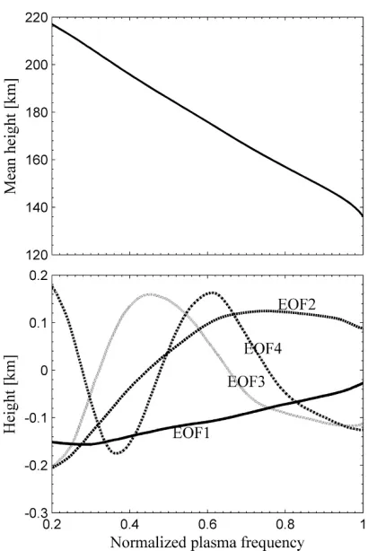
Fig. 2. EOF analysis results for the true ionospheric height of MGS elec-tron density profiles. The top and bottom panels indicate, respectively, the mean true height and the four leading EOFs vs. the normalized plasma frequency. plasma frequency, fp, and the corresponding electron den-sity, Ne, respectively, and the superscript asterisk denotes the normalized value.
Assuming that the electron density profile in the Martian topside ionosphere is a monotonically decreasing function, we can obtain a true height functionh(fp∗)by inverting the normalized profile fp∗(h). Thus, a sampled dataset ofh(fp∗)
is obtained for the EOF analysis (Wilks, 1995),
hj
function) and Aj k is the corresponding coefficient for the
jth true height function. The total number of EOFs, K,
is determined by the number of fpi∗. Ek(fpi∗)’s are
empiri-cally determined by diagonalizing the covariance matrix be-tween(hi’s−hi’s); i.e.Ek(fpi∗)is thekth orthonormalized
eigenvector of the covariance matrix. As shown by stan-dard mathematical analysis (see, e.g., Jolliffe, 2002), if we
project the datahj(fpi∗)onto the Ek(fpi∗)’s, then the
pro-jectionkAj kEk(fpi∗),(k=1,2, . . . ,K;M ≤K)
repre-sents the maximum possible fraction of the variability con-tained inhj(fpi∗). Therefore, the EOF series in Eq. (2)
con-verges most quickly in representing the true height dataset
hj(fpi∗). For instance, four leading terms Aj kEk(fpi∗),
(k=1,2,3,4)may represent 94% of the total variance of our true height dataset. Hence, in our ionogram inversion
we truncated the EOF series at K = 4. The mean height
and the four leading EOFs vs. the normalized plasma fre-quency are illustrated in Fig. 2. The beginning of fpi∗ is
chosen as 0.2 to make sure that all values of the true height are sampled adequately to give a statistically valid result, though the information of the true height at fpi∗ smaller than 0.2 will be lost. It is clearly seen that, in general, the mean height function represents the typical variation of the 5600 MGS electron density profiles. The larger rank EOF refers to the smaller scale variation. The different scales of the true height variations can be represented by different ranks of the EOF.
3.2 Ionogram inversion
It is assumed that the Martian ionosphere is horizontally stratified. For a vertical incidence radio wave with fre-quency f, the echo is reflected from the rangezr where
the plasma frequency fpequals f. In this case, the apparent range from the spacecraft tozris given by
z(f)= index; fS is the local plasma frequency at the spacecraft; z(fp)is the true range, and can be computed from the true height,
z(fp)=hS−h(fp), (4)
wherehS is the true height of the spacecraft. The integral function (Eq. (3)) has a unique solution under the assump-tion, as was made above, that the electron density distri-bution in the topside ionosphere of Mars has a monotonic profile.
In the integration of Eq. (3), we adopt the variable trans-formation, fp = f sinϕ, to avoid the infinite nat the
re-flection point. Then Eq. (3) becomes
Fig. 3. The inversion result for the MARSIS ionograms shown in Fig. 1. The solid curves show the true height profiles of the normalized plasma frequency calculated using the EOF-based inversion in Section 3. The crosses show the measured apparent data which corresponds to the scaled apparent data in Fig. 1. The circles show the apparent heights recalculated using Eq. (6).
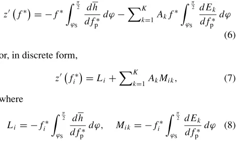
Noticing the relationship between the true range and the true height in Eq. (4), the following results may be obtained by substituting Eq. (2) into (5b)
zf∗= −f∗
π
2
ϕS
dh d fp∗ dϕ−
K k=1Akf
∗ π 2
ϕS
d Ek d fp∗ dϕ
(6)
or, in discrete form,
zfi∗
=Li+ K
k=1AkMi k, (7)
where
Li = −fi∗
π
2
ϕS
dh
d fp∗ dϕ, Mi k = −f ∗ i
π
2
ϕS
d Ek
d fp∗ dϕ (8)
can be calculated in advance;z(fi∗)is measured from the
ionogram with the scaling process in Section 2. Thus, the coefficients Ak are estimated by solving the matrix
equa-tion (Eq. (7)), and thefinal electron density profile is then obtained by Eq. (2). However, in most cases, the densities between the spacecraft and thefirst reflection point are not known. In order to carry out the inversion, we assume that
the electron density varies exponentially with height in the gap. The assumption used here, similar to that of Nielsenet al.(2006), Gurnettet al.(2008) and Morganet al.(2008), is also a good approximation but not a complete description.
In theory, the EOF series, the same as the polynomials used previously (such as the Taylor or shifted Chebyshev polynomials), can be used to expand any electron density profile in the Martian topside ionosphere. Moreover, the EOF series converges more quickly, especially when it is used to represent the electron density profile in the range of the MGS radio occultation data, because the EOF series is derived from the measured MGS radio occultation data.
4.
Results
X. HAN AND W. WAN: IONOGRAM INVERSION FOR MARSIS TOPSIDE SOUNDING 757
good, indicating that the inversion result is a good estima-tion of the true electron density distribuestima-tion because the so-lution of the inversion problem is unique, as we mentioned in Section 3.
In Fig. 3, the recalculated apparent heights match the measured ones well, whether the electron density profile is in the range of the MGS dataset or not, which indicates that the EOF expansion of the electron density profile, though not optimal, is near optimal when the four EOFs are ex-trapolated to apply at all points in the topside ionosphere of Mars. The good extrapolation inspires confidence in pro-cessing a large quantity of MARSIS ionograms using the method developed.
5.
Summary and Conclusions
The EOF-based inversion is developed from the tradi-tional polynomial analysis of Titheridge (1961, 1967a, b, 1969, 1975, 1988) and Huang and Reinisch (1982) where the prior polynomials, e.g., Taylor polynomials or shifted Chebyshev polynomials, have now been replaced with em-pirical orthogonal functions (EOFs). The new technique has been applied here to the data processing of the MARSIS ionograms, with EOFs retrieved from the MGS radio oc-cultation measurements. The results show the remarkable advantage that only a few EOFs are required to represent most of the variability of the original dataset, owing to the quick convergence of the EOF series. These results show that the EOF-based inversion provides a new tool for the analysis of MARSIS ionograms.
Acknowledgments. This work is supported by the Chinese Academy of Sciences (KZZD-EW-01-2), the National Important Basic Research Project (2011CB811405) and the National Sci-ence Foundation of China (41131066, 40974090). The iono-gram data of MARSIS is downloaded from website ftp://pds-geosciences.wustl.edu/mex/. The authors also acknowledge the State Key Laboratory of Lithospheric Evolution for partial sup-port.
References
Budden, K. G.,Radio Waves in the Ionosphere, Cambridge Univ. Press, Cambridge, U.K., 1961.
Chicarro, A., P. Martin, and R. Trautner, The Mars Express mission: An overview, inMars Express: A European Mission to the Red Planet, edited by A. Wilson, pp. 3–16, ESA Publ. Div., Noordwijk, Netherlands, 2004.
Ding, Z., B. Ning, W. Wan, and L. Liu, Automatic scaling of F2-layer parameters from ionograms based on the empirical orthogonal function
(EOF) analysis of ionospheric electron density,Earth Planets Space,59, 51–58, 2007.
Duru, F., D. A. Gurnett, D. D. Morgan, R. Modolo, A. F. Nagy, and D. Najib, Electron densities in the upper ionosphere of Mars from the ex-citation of electron plasma oscillations,J. Geophys. Res.,113, A07302, doi:10.1029/2008JA013073, 2008.
Gurnett, D. A., R. L. Huff, D. D. Morgan, A. M. Persoon, T. F. Averkamp, D. L. Kirchner, F. Duru, F. Akalin, A. J. Kopf, E. Nielsen, A. Safaeinili, J. J. Plaut, and G. Picardi, An overview of radar soundings of the Martian ionosphere from the Mars Express spacecraft,Adv. Space Res., 41, 1335–1346, doi:10.1016/j.asr.2007.01.062, 2008.
Huang, X. Q. and B. W. Reinisch, Automatic calculation of electron den-sity profiles from digital ionograms: 2. True height inversion of top-side ionograms with the profile-fitting method,Radio Sci.,17, 837–844, 1982.
Jackson, J. E., The reduction of topside ionograms to electron-density profiles,Proc. IEEE,57, 960–975, 1969.
Jolliffe, I. T.,Principal Component Analysis, 2nd Ed., Springer, 2002. Morgan, D. D., D. A. Gurnett, D. L. Kirchner, J. L. Fox, E. Nielsen,
and J. J. Plaut, Variation of the Martian ionospheric electron density from Mars express radar soundings,J. Geophys. Res.,113, A09303, doi:10.1029/2008JA013313, 2008.
Nielsen, E., Mars Express and MARSIS,Space Sci. Rev.,111, 245–262, 2004.
Nielsen, E., H. Zou, D. A. Gurnett, D. L. Kirchner, D. D. Morgan, R. Huff, R. Orosei, A. Safaeinili, J. J. Plaut, and G. Picardi, Observations of vertical reflections from the topside Martian ionosphere,Space Sci. Rev.,126, 373–388, doi:10.1007/s11214-006-9113-y, 2006.
Picardi, G.et al., MARSIS: Mars Advanced Radar for Subsurface and Ionosphere Sounding, inMars Express: A European Mission to the Red Planet, edited by A. Wilson, pp. 51–70, ESA Publ. Div., Noordwijk, Netherlands, 2004.
Reinisch, B. W. and X. Q. Huang, Automatic calculation of electron den-sity profiles from digital ionograms: 3. Processing of bottomside iono-grams,Radio Sci.,18, 477–492, 1983.
Titheridge, J. E., A new method for the analysis of ionospherich(f)
records,J. Atmos. Terr. Phys.,21, 1–12, 1961.
Titheridge, J. E., The overlapping-polynomial analysis of ionograms, Ra-dio Sci.,2, 1169–1175, 1967a.
Titheridge, J. E., Direct manual calculation of ionospheric parameters us-ing a sus-ingle-polynomial analysis,Radio Sci.,2, 1237–1254, 1967b. Titheridge, J. E., The single polynomial analysis of ionograms,Radio Sci.,
4, 41–51, 1969.
Titheridge, J. E., The relative accuracy of ionogram analysis techniques,
Radio Sci.,10, 589–599, 1975.
Titheridge, J. E., The real height analysis of ionograms: A generalized formulation,Radio Sci.,23, 831–849, 1988.
Whittaker, E. T. and G. N. Watson,A Course of Modern Analysis, Cam-bridge Univ. Press, CamCam-bridge, U.K., 1927.
Wilks, D. S.,Statistical Methods in the Atmospheric Sciences, Academic Press, San Diego, 1995.
Zou, H., E. Nielsen, J.-S. Wang, and X.-D Wang, Reconstruction of non-monotonic electron density profiles of the Martian topside ionosphere,
Planet. Space Sci.,58, 1391–1399, 2010.