R E S E A R C H
Open Access
A low computational complexity
normalized subband adaptive filter
algorithm employing signed regressor of
input signal
Mohammad Shams Esfand Abadi
*, Mohammad Saeed Shafiee and Mehrdad Zalaghi
Abstract
In this paper, the signed regressor normalized subband adaptive filter (SR-NSAF) algorithm is proposed. This algorithm is optimized byL1-norm minimization criteria. The SR-NSAF has a fast convergence speed and a low steady-state error similar to the conventional NSAF. In addition, the proposed algorithm has lower computational complexity than NSAF due to the signed regressor of the input signal at each subband. The theoretical mean-square performance analysis of the proposed algorithm in the stationary and nonstationary environments is studied based on the energy conservation relation and the steady-state, the transient, and the stability bounds of the SR-NSAF are predicated by the closed form expressions. The good performance of SR-NSAF is demonstrated through several simulation results in system identification, acoustic echo cancelation (AEC) and line EC (LEC) applications. The theoretical relations are also verified by presenting various experimental results.
Keywords: Normalized subband adaptive filter (NSAF), Mean-square performance, Signed regressor (SR)L1-norm
1 Introduction
Fast convergence rate and low computational complexity features are important issues for high data rate applications such as speech processing, echo cancelation, network echo cancelation, and channel equalization. The least-mean-squares (LMS) and the normalized LMS (NLMS) algo-rithms are useful for a wide range of adaptive filter applica-tions because of their low computational complexity. However, the performance of the LMS-type algorithms is corrupted when the input signals are colored [1,2].
To solve this problem, various approaches such as affine projection algorithm (APA) [3,4] and subband adaptive filter (SAF) algorithm have been proposed [5–7]. In [8], a new ver-sion of the SAF was developed based on a constrained optimization problem referred to as normalized SAF (NSAF). The filter update equation in [8] is similar to the update equation in [9,10], where the full band filters are updated in-stead of subfilters as in the conventional SAF structure [5].
To reduce the computational complexity of NSAF and APA, different methods were proposed. In [11], the selective partial update NSAF (SPU-NSAF) algorithm was presented where the filter coefficients are partially updated rather than the entire filter at every adaptation. In [12], the dynamic se-lection of NSAF (DS-NSAF) algorithm was introduced. In this algorithm, the number of subbands was optimally selected during each iteration. The fix selection NSAF (FS-NSAF) was also introduced in [13]. In this algorithm, a sub-set of subbands was selected during the adaptation.
There are some classes of adaptive filter algorithms that make use of the signum of either the error signal or the input signal, or both. These approaches have been applied to the LMS algorithm for the simplicity of im-plementation, enabling a significant reduction in compu-tational complexity [14–18]. The sign algorithm (SA) takes the signum of the error signal. This algorithm is particularly useful against impulsive interferences [19, 20]. But, in other cases, the convergence speed of the SA is slower than conventional one [21]. This approach was also successfully extended to the NSAF algorithm to es-tablish the sign SAF (SSAF) algorithm [22,23].
* Correspondence:[email protected]
Faculty of Electrical Engineering, Shahid Rajaee Teacher Training University, P.O.Box: 16785-163, Tehran, Iran
In the signed regressor LMS (SR-LMS), the signum of the input regressors is utilized. In this algorithm, the polar-ity of the input signal is used to adjust the filter coefficients, which requires no multiplications. The SR-LMS has a con-vergence speed and a steady-state error level that are only slightly inferior to those of the LMS algorithm for the same parameter setting [24]. To increase the convergence speed of SR-LMS, the signed regressor NLMS (SR-NLMS) was firstly proposed in [14]. Also, the modified version of this
algorithm (MSR-NLMS) was presented in [25]. The same
as SR-LMS, the SR-NLMS enjoys advantages similar to those of the NLMS algorithm. Due to the normalization factor, the steady-state error level does not depend on the input signal power [18]. Note that no multiplications are needed to calculate the normalization factor. But for highly colored input signal, the convergence speed of SR-NLMS is still low. On the other hand, there is no definition for cost function or solving the optimization problem to establish-ment of the signed regressor algorithms in the literature.
Due to the effective features of signed regressor adaptive algorithms (low computational complexity and close conver-gence speed to the conventional algorithm) and to increase the performance of the SR-NLMS algorithm, this paper pro-poses the signed regressor NSAF (SR-NSAF) algorithm. The SR-NSAF is established withL1-norm optimization. A
con-straint is imposed on the decimated filter output to force a posteriori error to become zero. This constraint guarantees the convergence of the algorithm. This algorithm utilizes the signum of the input regressors at each subband during the adaptation. Again, no multiplications are required for normalization factor at each subband. To improve the per-formance of the SR-NSAF, the modified SR-NSAF (MSR-NSAF) is also established. The proposed SR-NSAF and MSR-NSAF algorithms have lower computational complex-ity than the NSAF, SPU-NSAF, DS-NSAF, and FS-NSAF, while they have a fast convergence rate similar to the NSAF. In addition, the steady-state error level is also nearly close to the NSAF. For performance evaluation of any proposed adaptive algorithm, a theoretical analysis is essential [26]. Therefore, in the following, the energy conservation ap-proach [27] is applied to the SR-NSAF and the mean-square performance analysis of the proposed algorithms are studied in the stationary and nonstationary environ-ments. This approach does not need a white or Gaussian assumption for the input regressors. Based on this, the transient, the steady-state, and the stabil-ity bounds of the SR-NSAF and MSR-NSAF are ana-lyzed and closed form relations are derived.
What we propose in this paper can be summarized as follows:
The establishment of the SR-NSAF according to the proposed cost function. This algorithm utilizes the signum of the input regressors at each subband.
Furthermore, no multiplications are required for normalization factor at each subband.
Mean-square performance analysis of the SR-NSAF algorithm in the stationary and nonstationary
environments. The theoretical expressions for transient and steady-state performances of the SR-NSAF are extracted.
Analysis of the mean and mean-square stability bounds of the SR-NSAF and MSR-NSAF algorithms.
The performance of NSAF, SPU-NSAF, DS-NSAF, FS-NSAF, SR-NSAF, and MSR-NSAF are compared in convergence speed, steady-state error, and computational complexity features for system identification, acoustic echo cancelation, and line echo cancelation applications.
The theoretical expressions for transient, steady-state, and stability bounds are justified with various experiments.
The current paper is organized as follows. In Section II, the conventional NSAF is briefly reviewed. The proposed SR-NSAF and MSR-NSAF are presented in Section III. Section IV presents the mean square performance analysis of SR-NSAF. The theoretical stability bounds relations are given in Section V. In the following, the computational complexity of the proposed algorithm will be discussed. Finally, before concluding the paper, the usefulness of the introduced algorithms are demonstrated by presenting several experimental results.
Throughout the paper, the following notations are used:
|.| Norm of a scalar
‖.‖2 Squared Euclidean norm of a vector.
‖.‖1 L1-norm of a vector.
(.)T Transpose of a vector or a matrix.
E{.} Expectation operator.
sgn Sign function.
Tr(.) Trace of a matrix.
λmax The largest eigenvalue of a matrix. ℜ+
The set of positive real numbers.
Α⊗Β Kronecker product of matricesΑandΒ
ktk2Φ Φ-weighted Euclidean norm of a column vectortdefined astT
Φt.
diag(.) Has the same meaning as the MATLAB operator with the same name: if its argument is a vector, a diagonal matrix with the diagonal elements given by the vector argument results. If the argument is a matrix, its diagonal is extracted into a resulting vector.
vec(T) Creates anM2× 1 column vectortthrough stacking the columns of theM×MmatrixT.
vec(t) Creates anM×MmatrixTfrom theM2× 1 column vectort.
2 Background on NSAF
d nð Þ ¼xTð Þn woþv nð Þ ð1Þ
wherewois an unknownM-dimensional vector that we expect to estimate,v(n) is the measurement noise with varianceσ2
v andx(n) = [x(n),x(n−1),…,x(n−M+ 1)]T
denotes anM-dimensional input (regressor) vector. It is assumed thatv(n) is zero mean, white, Gaussian, and independent ofx(n). Figure1shows the structure of the NSAF [8]. In this figure,f0,f1,…,fN−1andg0,g1,…,gN −1, are analysis and synthesis filter unit impulse
responses of anNchannel orthogonal perfect
reconstruction critically sampled filter bank system.xi(n) anddi(n) are nondecimated subband signals. It is
important to note thatnrefers to the index of the original sequences, andkdenotes the index of the decimated sequences (k= floor(n/N)). The decimated output signal is defined asyi;DðkÞ ¼xTiðkÞwðkÞwherexi(k) = [xi(kN),
xi(kN−1),…,xi(kN−M+ 1)]Tandw(k) = [w0(k), w1(k), …,wM−1(k)]T. Also, the decimated subband error signal is
defined asei;DðkÞ ¼di;DðkÞ−xTiðkÞwðkÞ. The filter update
equation for NSAF can be stated as
wðkþ1Þ ¼wð Þ þk μX
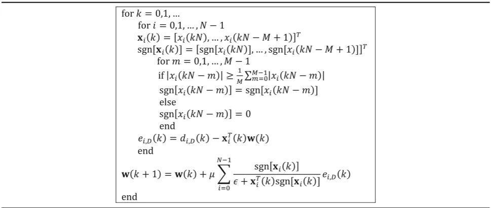
3 Sign regressor normalized subband adaptive filter(SR-NSAF)
Based on the principle of minimum disturbance, the SR-NSAF is formulated by the following optimization problem
minkwðkþ1Þ−wð Þk k1 ð3Þ
subject to theNconstraints (i= 0, 1,…,N−1) which are defined as
di;Dð Þ ¼k xTið Þk wðkþ1Þ ð4Þ
By applying the method of Lagrange multipliers, the following Lagrangian function is obtained
Jðwðkþ1ÞÞ ¼kwðkþ1Þ−wð Þk k1
¼0;we get the following relation as
sgn½wðkþ1Þ−wð Þk ¼X
N−1
i¼0
λixið Þk ð6Þ
In NSAF algorithm, if the magnitude responses of the analysis filters do not significantly overlap, the cross-correlation between two arbitrary subband signals is negligible compared to the auto-correlation [8]. There-fore, by multiplying xT
i ðkÞ on both sides of the above equation from the left and neglecting the crossterms, we obtain
xiTð Þk sgn½wðkþ1Þ−wð Þk ¼λikxið Þk k2 ð7Þ
By defining sgn(xi(k)) =Θi(k)xi(k), sgn[w(k+ 1)−w(k)] =Υ(k)[w(k+ 1)−w(k)], and multiplying sgn(xi(k)) on both sides of (7) from the left, we get
Θið Þk xið Þk xTið ÞΥk ð Þk ½wðkþ1Þ−wð Þk be approximately assumed white [26, 28]. Therefore, by displacing the matrices in (8) and using (4), we obtain
Υð ÞΘk ið Þk xið Þek i;Dð Þ ¼k λixið Þk kxið Þk k1 ð11Þ
Where kxiðkÞk1¼sgnðxTi ðkÞÞxiðkÞ . Now, by multiplying sgnðxT
i ðkÞÞ on both sides of (11) from the left, the Lagrange multipliers are given by
λi¼ sgn xTi ð Þk
Substituting (12) into (6) leads to
Υð Þk½wðkþ1Þ−wð Þk ¼X left and rearranging the diagonal matrices, the filter coefficients of the update equation for SR-NSAF is established as
whereμis again the step size and should be selected in the stability bound.1To avoid being divided by zero, it is
common that the denominator of the update equation is replaced byϵ+‖xi(k)‖1, whereϵis the regularization
parameter. Table1summarizes the SR-NSAF algorithm.
It is interesting to note that for N= 1, and f0= 1, the
SR-NSAF in (14) reduces to
wðnþ1Þ ¼wð Þ þn μ sgn½xð Þn
xð Þn
k k1 e nð Þ ð15Þ
which is the SR-NLMS algorithm [14]. In this case, the output error is given bye(n) =d(n)−xT(n)w(n).
In [25], the new version of SR-NLMS was proposed
based on clipping of the input signal. When the absolute value of the sample is larger than the average of the ab-solute values of the input samples, the clipped sample is used to update coefficients. The performance of SR-NSAF can be improved by applying the proposed idea in [25] in each subband. Therefore, the new version of SR-NSAF which is called modified SR-SR-NSAF (MSR-SR-NSAF) is established based on the procedure in Table2.
4 Mean square performance analysis of SR-NSAF in stationary environment
The filter coefficients update equation in SR-NSAF can be represented as
wðkþ1Þ ¼wð Þ þk μ sgn½Xð Þk FWð Þk FTeð Þ ðk 16Þ
whereFis theK×Nmatrix whose columns are the unit pulse responses of the channel filters of a critically sampled analysis filter bank,2F =[f0,f1,…,fN−1],X(k) is
theM×Kinput signal matrix which is defined as
Xð Þ ¼k ½xðkNÞ;xðkN−1Þ;…;xðkN−ðK−1ÞÞ ð17Þ
and
dð Þ ¼k ½d kNð Þ;d kNð −1Þ;…;d kNð −ðK−1ÞÞT ð18Þ
Also, (k)=[ϵI+diag {diag{FTXT(k) sgn[X(k)F]}}]−1, and
eð Þ ¼k dð Þk −XTð Þk wð Þk ð19Þ
is the error signal vector. In the theoretical convergence
analysis, we need to obtain the time evolution of the
Efkw~ðkÞk2Φg, wherew~ðkÞ ¼wo−wðkÞ is the
weight-error vector, and Φ is any Hermitian and positive-definite matrix. When Φ= I (Iis the identity matrix), the mean square deviation (MSD) and when Φ= R (R is the autocorrelation matrix of the input signal), the excess mean square error (EMSE) expressions are derived.
The weight error vector update equation for SR-NSAF can be written as
Substituting (21) into (20) yields
wðkþ1Þ ¼w~ð Þk−μ sgn½Xð Þk FWð Þk FTXTð Þkw~ð Þ þk vð Þk
ð22Þ
By taking the Φ-weighted norm from both sides of
(22), we obtain applying the expectation into both sides of (23), we obtain
Ekw~ðkþ1ÞkΦ2 ¼E kw~ð Þk k2Ψ
þμ2
EvTð Þk Yð Þk vð Þk ð26Þ
To simplify the recent relation, we need the
independence assumptions. The matrix X(k) is assumed
an independent and identically distributed sequence matrix [2, 27]. This assumption guarantees that w~ðkÞ is independent of bothΨandX(k). Therefore,
Table 3The computational complexity of NSAF and SR-NSAF
Ψ¼Φ−μΦEfZð Þk g−μEZTð Þk Φ þμ2
EZTð ÞΦk Zð Þk ð27Þ
The second term of the right hand side of (26) can be presented as
Applying the vec(.) operation on both sides of (25) and using vec(PΦQ) = (QT⊗P)vec(Φ) lead to defining the matrixPas
P¼I−μEZTð Þk I−μIEZTð Þk
Finally, (26) can be stated as
Enkw~ðkþ1Þk2ϕo¼E kw~ð Þk k2Pϕ
n o
þμ2σ2
vφTϕ ð35Þ
This equation is related tow~ð0Þas
Fig. 2Number of multiplications versus the filter length for NSAF, DS-NSAF, FS-NSAF, SPU-NSAF and proposed SR-NSAF withN= 8 Table 4Computational complexity of the family of NSAF
E kw~ð Þk k2ϕ
n o
¼E kw~ð Þ0 k2Pkϕ
n o
þμ2σ2
vφT IþPþ…þPk−1
ϕ
ð36Þ
By substituting R for Φ, and defining r =vec(R), the transient behavior of SR-NSAF can be predicted by (35). From this recursion, we can obtain EMSE, whenkgoes to infinity. Therefore, the EMSE in the steady-state can be stated as
EMSE¼μ2σ2vφTðI−PÞ−1r ð37Þ
The MSE and the EMSE are related as
MSE¼EMSEþσ2v ð38Þ
Also, the steady state mean square coefficient
deviation (MSD) is given by
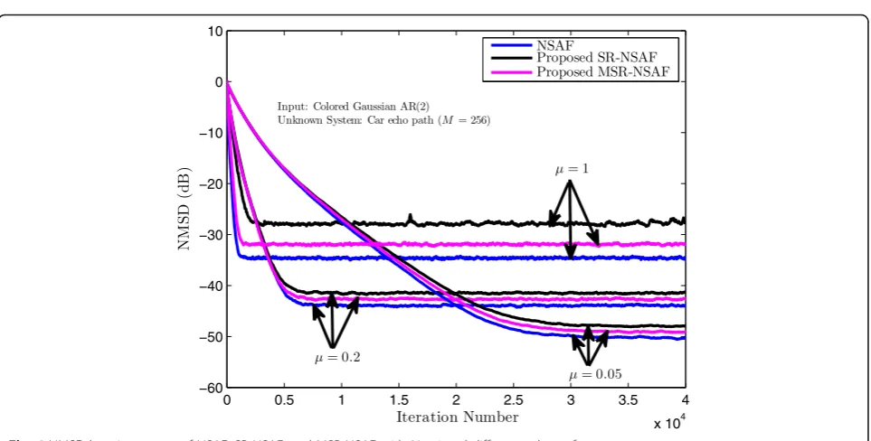
Fig. 4NMSD learning curves of NSAF, SR-NSAF, and MSR-NSAF withN= 4 and different values ofμ
MSD¼μ2σ2vφTðI−PÞ−1vecð ÞI ð39Þ
It is important to note that selectingF = Iand N=K= 1 lead to the performance analysis of SR-NLMS and
MSR-NLMS algorithms, which was not presented in [14,
25]. This analysis can be successfully extended to
non-stationary environment. InAppendix1, the mean-square
performance analysis of the SR-NSAF is presented in the nonstationary environment.
5 Mean and mean-square stability of the SR-NSAF Taking the expectation from both sides of (22) leads to
Efw~ðkþ1Þg ¼Efw~ð Þk −μ sgn½Xð Þk FWð Þk FT XTð Þk w~ð Þ þk vð Þk
g
ð40Þ
From (40), the convergence to the mean of the SR-NSAF is guaranteed for anyμthat satisfies
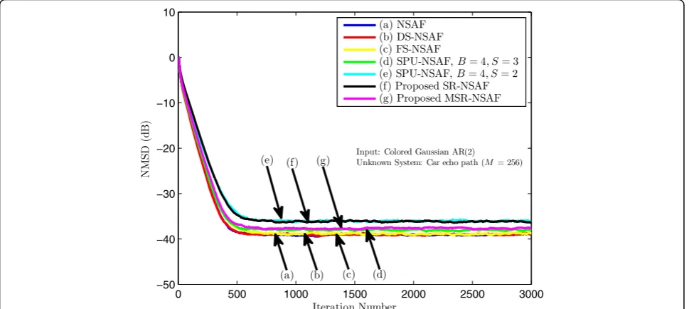
Fig. 6NMSD learning curves of NSAF, DS-NSAF, FS-NSAF, SPU-NSAF, SR-NSAF, and MSR-NSAF withN= 8 andμ= 0.5
μ< 2
λmax E sgn½Xð Þk FWð Þk FTXTð Þk
ð41Þ
Equation (35) is stable if the matrix P is stable
[27]. From (31), we know that P = I−μM +μ2N,
where M =E{ZT(k)}⊗I + I⊗E{ZT(k)}, and N = E{ZT(k)⊗ZT(k)}. The condition on μ to guarantee the convergence in the mean-square sense of the SR-NSAF algorithms is
0<μ< min 1
λmax M−1N
; 1
maxλð ÞH∈ℜþ
( )
ð42Þ
whereH¼
1
2M −12N
I 0
.
6 Computational complexity
Table 3 compares the computational complexity of the
NSAF and SR-NSAF algorithms. This table shows that the number of multiplications in SR-NSAF is lower than
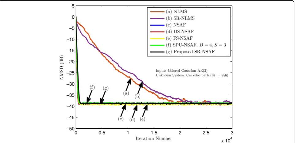
Fig. 8NMSD learning curves of NLMS, SR-NLMS, NSAF, DS-NSAF, FS-NSAF, SPU-NSAF, and SR-NSAF withN= 8
NSAF. Table 4 summarizes the number of multiplica-tions at each iteration for different NSAF algorithms. In this table, M, N, K, B, S, L, Ns, and N(k) are the filter length, the number of subbands, the length of channel filters, the number of blocks, the number of blocks to update, the length of blocks, the number of selected sub-bands (fix), and the number of selected subsub-bands (dy-namic), respectively. For NSAF, the exact computational complexity of this algorithm is 3M+ 3NK+ 1 multiplica-tions [11]. From [11], we obtain that the computational
complexity of SPU-NSAF is 2M+SL+ 3NK+ 1
multipli-cations. In comparison with NSAF, the reduction in
number of multiplications is M−SL, which is
consider-able for large values of M. Also, the DS-NSAF needs ð1
þ2NNðkÞÞMþ3NKþN multiplications [12]. Due to the selection of subbands during the adaptation, the number of multiplications will be reduced in DS-NSAF. The exact number of multiplications in FS-NSAF is 2Mþ ðNs
NÞ
Mþ3NKþ1. Compared with SPU-NSAF, FS-NSAF, and
DS-NSAF algorithms, the proposed SR-NSAF algorithm
needs 2M multiplications less than NSAF algorithm.
Figure 2 compares the number of multiplications versus
the filter length for NSAF, FS-NSAF, DS-NSAF, SPU-NSAF (B= 4, S= 1, 2, 3), and proposed SR-NSAF withN= 8. As we can see, the number of multiplications in SR-NSAF is significantly lower than other algorithms.
7 Simulation results
We demonstrated the performance of the proposed algorithm by several computer simulations in a system identification (SI), acoustic echo cancelation (AEC) and line echo cancelation (LEC) setups. The impulse
response of the car echo path with 256 taps (M= 256)
has been used as an unknown system in the experiment
[29] (Fig. 3). The filter bank used in the NSAF
algorithms was the extended lapped transform (ELT) (N
= 2, 4, and 8) [11, 30]. In all simulations, we show the normalized mean square deviation (NMSD),E½kwok−wwoðkk2Þk2,
which is evaluated by ensemble averaging over 20 independent trials.
7.1 System identification: AR(2) input signal
In this experiment, the input signal is an AR(2) signal generated by passing a zero-mean white Gaussian noise
through a second-order system TðzÞ ¼ 1
1−0:1z−1−0:8z−2. An
additive white Gaussian noise was added to the system output, setting the signal-to-noise ratio (SNR) to 30 dB.
Figure 4 compares the convergence of the NSAF,
SR-NSAF, and MSR-NSAF algorithms with N= 4 for
differ-ent step sizes (1, 0.2, and 0.05). As we can see, for large values of the step size, the fast convergence rate and
Fig. 9NMSD learning curves for tracking performance of NSAF, DS-NSAF, FS-NSAF, SPU-NSAF, SR-NSAF, and MSR-NSAF withN= 8 andμ= 0.5 Table 5Number of multiplications for various NSAF algorithms
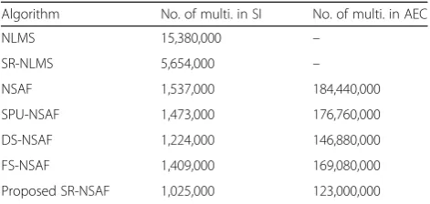
until convergence in SI and AEC applications
Algorithm No. of multi. in SI No. of multi. in AEC
high steady-state error are occurred and small step size leads to the slow convergence rate and a low
steady-state error. Figure 5 shows the performance of the
SR-NSAF, MSR-SR-NSAF, and conventional NSAF for the
number of subbandsN= 4 and 8. The step-size was set
to μ= 0.05. By increasing the number of subbands in all algorithms, the convergence rate is improved and the computational complexity is also increased. The results
show that the SR-NSAF, and MSR-NSAF algorithms have close performance to the conventional NSAF. Fur-thermore, the computational complexity of SR-NSAF and MSR-NSAF is lower than NSAF.
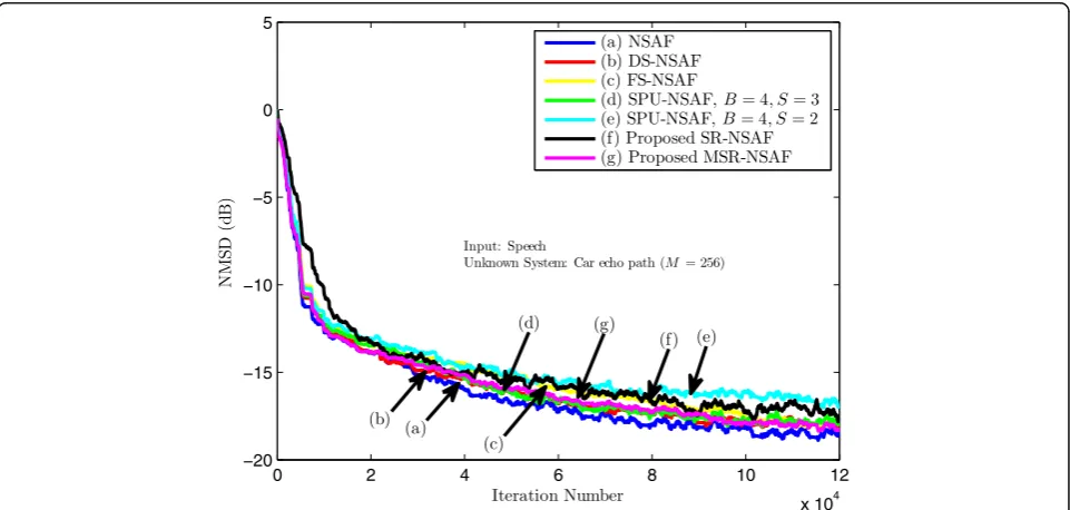
The performance of the proposed SR-NSAF and MSR-NSAF algorithms have been compared with other MSR-NSAF algorithms in Fig.6. These algorithms are NSAF [8],
DS-NSAF [12], FS-NSAF [13], and SPU-NSAF algorithm in
Fig. 11NMSD learning curves of NSAF, DS-NSAF, FS-NSAF, SPU-NSAF, SR-NSAF, and MSR-NSAF withN= 4. Under-modeling scenario, speech input signal
[11]. Eight subbands have been used (N= 8) and the
step-size was set toμ= 0.5. In FS-NSAF, the number of
selected subbands (Ns) out of the number of subbands
(N) was set to 4. For SPU-NSAF algorithm, the number
of blocks (B) was set to 4 and the number of blocks to update (S) was set 3 and 2. As we can see, the proposed SR-NSAF and MSR-NSAF have a comparable perform-ance to the family of NSAF in terms of the convergence
speed and the steady-state error. In addition, the compu-tational complexity of the introduced algorithms are lower than other algorithms.
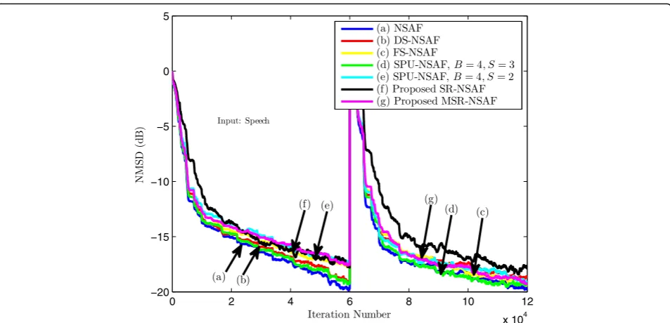
In Fig. 7, the step-size was set to 0.5 in NSAF algo-rithm and to make the comparison fair, the step-sizes for other NSAF algorithms were chosen to get ap-proximately the same steady-state NMSD as NSAF. For DS-NSAF and FS-NSAF, the step-size was set to
Fig. 13Impulse response of the line echo path
Fig. 15Error signals with NSAF, SR-NSAF, and MSR-NSAF algorithms
0.5. In SPU-NSAF, the step-sizes for S= 2 and S= 3 were set to 0.32 and 0.42, respectively. Finally, this value for SR-NSAF was set to 0.32 and for MSR-NSAF, the step-size was set to 0.4. The NMSD learn-ing curves show that the SR-NSAF and MSR-NSAF have a comparable performance with those of the
family of NSAF algorithms. In Fig. 8, we compared
the NMSD learning curves of NLMS and SR-NLMS algorithms with the family of NSAF algorithms. For
this simulation, the number of multiplications until
convergence was also presented in Table 5. This table
indicates that the number of multiplications in SR-NSAF is 1025000 which is significantly lower than other algorithms.
For tracking performance analysis, we consider a system to identify the two unknown filters with
M= 200, whose z-domain transfer functions are
given by
W1ð Þ ¼z
X99
n¼0
z−n− X
M−1
n¼100
z−n ð43Þ
and
W2ð Þ ¼z −
X
M−1
n¼0
z−n ð44Þ
where the transfer function of optimum filter coefficients will be W1(z) for n≤5 × 10³ and the
transfer function of optimum filter coefficients will
beW2(z) for 5 × 10³≤n≤10 × 103. Figure9compares the
tracking performance of SR-NSAF and MSR-NSAF with other NSAF algorithms. The number of subbands and the step-size were set to 8 and 0.5. As we can see, the SR-NSAF and MSR-SR-NSAF have a close performance to the conventional NSAF algorithm.
7.2 Acoustic echo cancelation (AEC): speech input signal For AEC setup, we consider both the exact and under-modeling scenarios. For the under-under-modeling scenario, the NMSD is calculated by padding the tap-weight
Fig. 19Simulated and theoretical MSE learning curves of SR-NSAF for different values ofN
vector of the adaptive filter withM−Jzeros (J=length of adaptive filter which is shorter than that of the unknown system in this case) [31]. In the exact-modeling scenario, the echo path is truncated to the first 128 tap weights [before the dotted line in Fig. 3]; in the under-modeling scenario, the length of the echo path is set to 256. For both scenarios, the length of all the adaptive filters is set to 128. Speech input signal is used as input signal for AEC setup [26].
Figures 10 and 11 compare the performance of
proposed SR-NSAF and MSR-NSAF algorithms with other NSAF algorithms in exact and under modeling
scenarios. The number of subbands (N) was set to 4.
In FS-NSAF, the number of selected subbands (Ns)
out of the number of subbands (N) was set to 2. As
we can see, the proposed SR-NSAF and MSR-NSAF have a comparable performance to the family of NSAF in terms of the convergence speed and the steady-state misalignment with lower computational
complexity. Table 5 shows the number of
multiplica-tions until convergence for different NSAF algorithms. This table indicates that the proposed SR-NSAF has significantly lower computational complexity than other algorithms.
The tracking capability is examined by shifting the acoustic impulse response to the right by 10 samples at
a certain time step. Figure 12 compares the tracking
performance of SR-NSAF and MSR-NSAF with other NSAF algorithms in exact modeling scenario. The num-ber of subbands was set to 4. As we can see, the SR-NSAF and MSR-SR-NSAF have close performance to the conventional NSAF algorithm.
7.3 Line echo cancelation
In communications over phone lines, a signal traveling from a far-end point to a near-end point is usually reflected in the form of an echo at the near-end due to mismatches in circuity. The purpose of a line echo canceller (LEC) is to eliminate the echo from a received
signal. Figure 13 shows the impulse response sequence
of a typical echo path which was taken from G168 Fig. 22Simulated and theoretical NMSD learning curves of SR-NSAF for different values ofμ
standard [32]. Figure 14 shows the far-end signal from real speech and echo signal (page 347 in [33]).
In this simulation, the length of the adaptive filter
is 128. Figure 15 shows the error signals based on
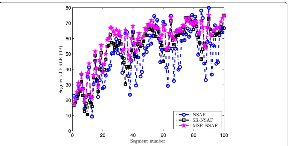
NSAF, SR-NSAF, and MSR-NSAF algorithms. The number of subbands, and the step-size were set to 4 and 0.5, respectively. As we can see, SR-NSAF and MSR-NSAF have close error performance to NSAF algorithm. Furthermore, the computational complex-ity of SR-NSAF and MSR-NSAF is considerably lower than that of NSAF. Also, to measure the effectiveness of the proposed algorithms, we have computed the echo return loss enhancement (ERLE). The ERLE is obtained by evaluating the difference between the powers of the echo and the error signal. The segmental ERLE estimates were obtained by averaging over 140 samples. The segmental ERLE curves for the measured speech and echo signals
were shown in Fig. 16. This figure illustrates that
the proposed algorithms and conventional NSAF have comparable ERLE performance.
7.4 Performance in nonstationary environment
Figure17presents the NMSD learning curves of NSAF and
SR-NSAF in nonstationary environment. The unknown system changes according to the random walk model. We assume an independent and identically distributed se-quence for q(n) with autocorrelation matrix Q¼σ2
qI [27]. The number of subbands and the step-size were set to 8 and 0.5 and different values forσ2
q(0:00025σ2vand 0:0025σ2v) have been chosen in simulations. This figure shows that the steady-state NMSD in nonstationary environment is larger than stationary environment. We also observe that the con-vergence speed of SR-NSAF is faster than NSAF for both values of σ2
q. To justify these results, we presented Fig.18. This figure shows the simulated NMSD values as a function of the step-size for NSAF and SR-NSAF in stationary and nonstationary environments. The step-size changes from 0. 1 to 1. The results show that in the stationary environment, the simulated NMSD values for NSAF are lower than SR-NSAF. In the nonstationary environment, there is an optimum value for the step-size that minimizes NMSD. This fact can be seen forσ2
q¼0:00025σ2v. Since the NMSD Table 6Stability bounds of the SR-NSAF and MSR-NSAF for different values ofN
Algorithm 2
learning curves were obtained forμ equal to 0.5, the SR-NSAF has slightly better performance than SR-NSAF in non-stationary environment.
7.5 Theoretical performance analysis
7.5.1 Simulation results for transient performance
The theoretical results presented in this paper are confirmed by several computer simulations for a
system identification setup. In this case, the unknown
system has 16 randomly selected taps. Figures19and20
show the simulated and theoretical MSE learning curves of SR-NSAF algorithm. The simulated learning curves are obtained by ensemble averaging over 100 independent trials. The theoretical learning curve are
obtained from (36). In Fig. 19, different values for N
have been selected. The good agreement between
Fig. 26Simulated and theoretical steady-state MSE of SR-NSAF withN= 2, 4, and 8 as a function of the step-size
theoretical and simulated learning curves is observed.
Figure 20 presents the results for different values of
μ. As we can see, there is good a agreement between
simulated and theoretical learning curves. In Figs. 21
and 22, the simulated and theoretical NMSD learning
curves were presented. The same as Figs. 19 and 20,
different values for N and μ were chosen. Again, a
good agreement can be seen in both figures. Figure 23
presents the theoretical and simulated MSE, MSD, and EMSE learning curves for SR-NSAF algorithm.
Good agreement between simulated and theoretical learning curves is observed.
7.5.2 Simulation results for stability bounds
Table 6 shows the theoretical values of the mean and
mean square stability bounds of SR-NSAF and MSR-NSAF algorithms. These values were obtained from (41) and (42). To justify these values, the simulated steady-state values of MSE were obtained. The steady-steady-state MSE is obtained by averaging over 500 steady-state sam-ples from 500 independent realizations for each value of μ for a given algorithm. The step-size (μ) changes from 0.05 toμmax. Figures24and 25show the results for
dif-ferent values ofN. As we can see, the theoretical values
for μmaxfrom Table 6 show good estimation of the
sta-bility bounds of SR-NSAF and MSR-NSAF algorithms. In [25], it was shown that the stability bound of MSR-NLMS is larger than that of SR-MSR-NLMS. It is interesting to note that this observation can be seen for the pro-posed algorithms. We observe that the stability bound of MSR-NSAF is larger than that of SR-NSAF algorithm.
7.5.3 Simulation results for steady-state performance
Figures 26 and 27 show the theoretical and simulated
steady-state MSE values of SR-NSAF and MSR-NSAF al-gorithms as a function of the step-size. The step-size (μ) changes from 0.05 to 1. The theoretical steady-state MSE values are obtained from (38). As we can see, there is good agreement between simulated and theoretical steady-state MSE values in both figures. For large values of the step-size, the agreement is slightly devi-ated. These figures show that the steady-state MSE
values for MNSAF are lower than those of SR-NSAF. This fact was also obtained for SR-NLMS and
MSR-NLMS algorithms in [25].
7.5.4 Theoretical results in nonstationary environment The theoretical and simulated NMSD learning curves in nonstationary environment were presented in Fig.
28. The theoretical learning curves were obtained
from (47). The number of subbands and the step-size
were set to 8 and 0.5. Various values for σ2
q (0:00025
σ2
v, 0:0025σ2v, and 0:025σ2v) have been selected in this simulation. Good agreement between the simulated and theoretical learning curves is observed in
nonsta-tionary environment. In Fig. 29, the simulated and
theoretical steady-state NMSD as a function of the step-size have been shown. The theoretical values were obtained from (49). This figure shows that there is an optimum step-size which minimizes the steady-state NMSD in nonstationary environment.
8 Conclusion
In this paper, the NSAF algorithm with signed regressor of input signal was established. The optimization problem was formulated by L1-norm minimization. The result of this
optimization leads to the sign operation on the input regressors at each subband. The computational complexity of the proposed SR-NSAF was lower than previous NSAF family while it had close convergence performance to the NSAF. Therefore, the SR-NSAF is a suitable candidate for many applications. To increase the performance of SR-NSAF, the MSR-NSAF was introduced. The performance
of the SR-NSAF was confirmed by several computer simu-lations in SI, AEC, and LEC applications. Also, the theoret-ical mean-square performance analysis and the stability bound of the proposed algorithms were studied and con-firmed by different experiments.
9 Endnotes
1
The theoretical stability bound of SR-NSAF is presented in Section VI. These values are justified in Section VIII
2
Kis the length of the channel filters.
10 Appendix
10.1 The theoretical relations in nonstationary environment
In the nonstationary environment, the unknown system (wo) is assumed time-variant which is changed according to the following random walk model [27,33].
woðkþ1Þ ¼woð Þ þk qð Þk ð45Þ
where the random sequence ofq(k) is a zero mean, an independent and identically distributed sequence with autocorrelation matrixQ=E{q(k)qT(k)} and independent ofx(kN) andv(k) [33]. Now by definingw~ðkÞ ¼woðkÞ−
wðkÞ, the weight error vector update equation can be expressed as
~
wðkþ1Þ ¼w~ð Þk
þqð Þk −μ sgn½Xð Þk FWð Þk FTeð Þk ð46Þ
By taking the Φ-weighted norm from both sides of
(46), then expectation, and following the same approach for stationary environment, we get
E kw~ðkþ1Þk2ϕ
When k goes to infinity, the steady-state EMSE in
nonstationary environment is given by
EMSE¼μ2σ2vφTðI−PÞ−1r
þTrQvecðI−PÞ−1r ð48Þ
and the steady-state MSD is obtained as
MSD¼μ2σ2vφTðI−PÞ−1vecð ÞI
þTrQvecðI−PÞ−1vecð ÞI ð49Þ
It is important to note that there is an optimal value for the step-size that minimizes the steady-state EMSE in the nonstationary environment [33] (Chapter 7). This effect comes from the second term in (48). In this term, the inverse of the step-size (μ−1) will appear, which has different effects on EMSE. For large values of the
step-size, this term will be small and the effect of the nonsta-tionary environment on EMSE will be small and the per-formance will be similar to the stationary case (Fig.29). For small values of the step-size, this effect will be large and the EMSE will be large. Therefore, there is an opti-mal value for the step-size that minimizes EMSE in non-stationary environment. More explanations about this issue can be found in [33].
Acknowledgements
The authors would like to thank Shahid Rajaee Teacher Training University (SRTTU) for financially support.
Funding
This work was financially supported by Shahid Rajaee Teacher Training University (SRTTU).
Authors’contributions
Due to the effective features of signed regressor adaptive algorithms (low computational complexity and close convergence speed to the conventional algorithm) and to increase the performance of the SR-NLMS algorithm, this paper proposes the signed regressor NSAF (SRNSAF) algorithm. The SR-NSAF is established withL1-norm optimization. A constraint is imposed on the
decimated filter output to force a posteriori error to become zero. This constraint guarantees the convergence of the algorithm. This algorithm utilizes the signum of the input regressors at each subband during the adaptation. Again, no multiplications are required for normalization factor at each subband. To improve the performance of the SR-NSAF, the modified SR-NSAF (NSAF) is also established. The proposed SR-NSAF and MSR-NSAF algorithms have lower computational complexity than the MSR-NSAF, SPU-NSAF, DS-SPU-NSAF, and FS-SPU-NSAF, while they have a fast convergence rate similar to the NSAF. In addition, the steady-state error level is also nearly close to the NSAF. For performance evaluation of any proposed adaptive algorithm, a theoretical analysis is essential [33]. Therefore, in the following, the energy conservation approach [27] is applied to the SR-NSAF and the mean-square performance analysis of the proposed algorithms are studied in the stationary and nonstationary environments. This approach does not need a white or Gaussian assumption for the input regressors. Based on this, the transient, the steady-state, and the stability bounds of the SR-NSAF and MSR-NSAF are analyzed and closed form relations are derived.
Competing interests
The authors declare that they have no competing interests.
Publisher’s Note
Springer Nature remains neutral with regard to jurisdictional claims in published maps and institutional affiliations.
Received: 28 September 2017 Accepted: 15 March 2018
References
1. S Haykin,Adaptive Filter Theory, 4th edn. (Prentica-Hall, 2002) 2. AH Sayed,Adaptive Filters(Wiley, 2008)
3. K Ozeki, T Umeda, An adaptive filtering algorithm using an orthogonal projection to an affine subspace and its properties. Electron Commun Jpn 67-A, 19–27 (1984)
4. M Muneyasu, T Hinamoto, A realization of TD adaptive filters using affine projection algorithm. J Franklin Inst335(7), 1185–1193 (1998)
5. A Gilloire, M Vetterli, Adaptive filtering in subbands with critical sampling: Analysis, experiments, and application to acoustic echo cancellation. IEEE Trans. Signal Process40, 1862–1875 (1992)
6. K-A Lee, W-S Gan, SM Kuo,Subband Adaptive Filtering: Theory and Implementation(Wiley, Hoboken, 2009)
7. MSE Abadi, S Kadkhodazadeh, A family of proportionate normalized subband adaptive filter algorithms. J Franklin Inst348(2), 212–238 (2011) 8. KA Lee, WS Gan, Improving convergence of the NLMS algorithm using
9. M de Courville, P Duhamel, Adaptive filtering in subbands using a weighted criterion. IEEE Trans Signal Process46, 2359–2371 (1998)
10. SS Pradhan, VE Reddy, A new approach to subband adaptive filtering. IEEE Trans Signal Process47, 655–664 (1999)
11. MSE Abadi, JH Husøy, Selective partial update and set-membership subband adaptive filters. Signal Process.88, 2463–2471 (2008)
12. SE Kim, YS Choi, MK Song, WJ Song, A subband adaptive filtering algorithm employing dynamic selection of subband filters. IEEE Signal Process Lett 17(3), 245–248 (2010)
13. MK Song, SE Kim, YS Choi, WJ Song, Selective normalized subband adaptive filter with subband extension. IEEE Trans Circuits Syst II: EXPRESS BRIEFS 60(2), 101–105 (2013)
14. J Nagumo, A Noda, A learning method for system identification. IEEE Trans. Automat. Contr.12, 282–287 (1967)
15. DL Duttweiler, Adaptive filter performance with nonlinearities in the correlation multipliers. IEEE Trans Acoust Speech Signal Process30(8), 578– 586 (1982)
16. A Gersho, Adaptive filtering with binary reinforcement. IEEE Trans. Inform. Theory30(3), 191–199 (1984)
17. WA Sethares, Adaptive algorithms with nonlinear data and error functions. IEEE Trans Signal Process40(9), 2199–2206 (1992)
18. S Koike, Analysis of adaptive filters using normalized signed regressor LMS algorithm. IEEE Trans Signal Process47(10), 2710–2723 (1999)
19. VJ Mathews, SH Cho, Improved convergence analysis of stochastic gradient adaptive filters using the sign algorithm. IEEE Trans Acoust Speech Signal Process35(4), 450–454 (1987)
20. P Wen, S Zhang, J Zhang, A novel subband adaptive filter algorithm against impulsive noise and it’s performance analysis. Signal Process.127(10), 282– 287 (2016)
21. TMCM Classen, WFG Mecklenbraeuker, Comparsion of the convergence of two algorithms for adaptive FIR digital filters. IEEE Trans Acoust Speech Signal Process29(6), 670–678 (1981)
22. J Ni, F Li, Variable regularisation parameter sign subband adaptive filter. Electron. Lett.64, 1605–1607 (2010)
23. J Shin, J Yoo, P Park, Variable step-size sign subband adaptive filter. IEEE Signal Process Lett20, 173–176 (2013)
24. NJ Bershad, Comments on‘comparison of the convergence of two algorithms for adaptive FIR digital filters. IEEE Trans Acoust Speech Signal Process33(12), 1604–1606 (1985)
25. K Takahashi, S Mori, inProc. ICCS/ISITA. A new normalized signed regressor LMS algorithm (Singapore, 1992), pp. 1181–1185
26. J Ni, F Li, A variable step-size matrix normalized subband adaptive filter. IEEE Trans Audio Speech Lang Process18, 1290–1299 (2010)
27. H-C Shin, AH Sayed, Mean-square performance of a family of affine projection algorithms. IEEE Trans Signal Process52(1), 90–102 (2004) 28. JJ Jeong, SH Kim, G Koo, SW Kim, Mean-square deviation analysis of
multiband-structured subband adaptive filter algorithm. IEEE Trans Signal Process64(4), 985–994 (2016)
29. K Dogancay, O Tanrikulu, Adaptive filtering algorithms with selective partial updates. IEEE Trans Circuits Syst II Analog Digit Signal Process48, 762–769 (2001) 30. H Malvar,Signal Processing with Lapped Transforms(Artech House, 1992) 31. C Paleologu, J Benesty, S Ciochina, A variable step-size affine projection
algorithm designed for acoustic echo cancellation. IEEE Trans Audio Speech Lang Process16, 1466–1478 (2008)