Model based control of exhaust gas recirculation valves and estimation of spring torque

University of Windsor University of Windsor

Scholarship at UWindsor

Scholarship at UWindsor

Electronic Theses and Dissertations Theses, Dissertations, and Major Papers

2010

Model based control of exhaust gas recirculation valves and

Model based control of exhaust gas recirculation valves and

estimation of spring torque

estimation of spring torque

Nazila Rajaei

University of Windsor

Follow this and additional works at: https://scholar.uwindsor.ca/etd

Recommended Citation Recommended Citation

Rajaei, Nazila, "Model based control of exhaust gas recirculation valves and estimation of spring torque" (2010). Electronic Theses and Dissertations. 7866.

https://scholar.uwindsor.ca/etd/7866

This online database contains the full-text of PhD dissertations and Masters’ theses of University of Windsor students from 1954 forward. These documents are made available for personal study and research purposes only, in accordance with the Canadian Copyright Act and the Creative Commons license—CC BY-NC-ND (Attribution, Non-Commercial, No Derivative Works). Under this license, works must always be attributed to the copyright holder (original author), cannot be used for any commercial purposes, and may not be altered. Any other use would require the permission of the copyright holder. Students may inquire about withdrawing their dissertation and/or thesis from this database. For additional inquiries, please contact the repository administrator via email

Model Based Control of

Exhaust Gas Recirculation Valves

and Estimation of Spring Torque

By

Nazila Rajaei

A Thesis

Submitted to the Faculty of Graduate Studies

through the Department of Electrical and Computer

Engineering in Partial Fulfillment of the Requirements

for the Degree of Master of Applied Science at

The University of Windsor

Windsor, Ontario, Canada

2010

1*1

Published Heritage Branch

395 Wellington Street Ottawa ON K1A 0N4 Canada

Bibliotheque et Archives Canada Direction du

Patrimoine de Pedition 395, rue Wellington OttawaONK1A0N4 Canada

Your file Votre reference ISBN: 978-0-494-62735-8 Our file Notre reference ISBN: 978-0-494-62735-8

NOTICE: AVIS:

The author has granted a

non-exclusive license allowing Library and Archives Canada to reproduce, publish, archive, preserve, conserve, communicate to the public by

telecommunication or on the Internet, loan, distribute and sell theses

worldwide, for commercial or non-commercial purposes, in microform, paper, electronic and/or any other formats.

L'auteur a accorde une licence non exclusive permettant a la Bibliotheque et Archives Canada de reproduire, publier, archiver, sauvegarder, conserver, transmettre au public par telecommunication ou par I'lnternet, preter, distribuer et vendre des theses partout dans le monde, a des fins commerciales ou autres, sur support microforme, papier, electronique et/ou autres formats.

The author retains copyright ownership and moral rights in this thesis. Neither the thesis nor substantial extracts from it may be printed or otherwise reproduced without the author's permission.

L'auteur conserve la propriete du droit d'auteur et des droits moraux qui protege cette these. Ni la these ni des extraits substantiels de celle-ci ne doivent etre imprimes ou autrement

reproduits sans son autorisation.

In compliance with the Canadian Privacy Act some supporting forms may have been removed from this thesis.

Conformement a la loi canadienne sur la protection de la vie privee, quelques formulaires secondaires ont ete enleves de cette these.

While these forms may be included in the document page count, their removal does not represent any loss of content from the thesis.

Bien que ces formulaires aient inclus dans la pagination, il n'y aura aucun contenu manquant.

1+1

DECLARATION OF PREVIOUS PUBLICATION

This thesis includes 2 original papers that have been previously published/accepted for

publication:

Thesis chapter

Chapter 4,5

Chapter 4,6

Paper title

"Spring TorqueEstimation in an Electronic Throttle Valve",IEEE VPPC Conference, 2010.

Publication status

Published

Accepted

I certify that I have obtained a written permission from the copyright owner(s) to include

the above published material(s) in my thesis. I certify that the above material describes

work completed during my registration as graduate student at the University of Windsor.

I declare that, to the best of my knowledge, my thesis does not infringe upon anyone's

copyright nor violate any proprietary rights and that any ideas, techniques, quotations, or

any other material from the work of other people included in my thesis, published or

otherwise, are fully acknowledged in accordance with the standard referencing practices.

Furthermore, to the extent that I have included copyrighted material that surpasses the

bounds of fair dealing within the meaning of the Canada

Copyright Act, I certify that I have obtained a written permission from the copyright

owner(s) to include such material(s) in my thesis.

I declare that this is a true copy of my thesis, including any final revisions, as approved

by my thesis committee and the Graduate Studies office, and that this thesis has not been

ABSTRACT

Exhaust Gas Recirculation (EGR) valves have been used in diesel engine operation to

reduce NOx emissions. In EGR valve operation, the amount of exhaust gas re-circulating

back into the intake manifold is controlled through the open position of the valve plate to

keep the combustion temperature lower for NOx emission reduction. Most of the control

methods do not provide sufficient control accuracy on the valve position and the response

time. Here, the model of a motor driven EGR valve is first identified through experiments

and then the Generalized Predictive Control (GPC) method is applied to control the plate

position of the valve. At the next step, to have a faster and more accurate control of the

valve the torque generated by the spring connected inside the valve is estimated. The

spring torque is considered as an external disturbance torque and three filters: Kalman,

DEDICATION

/ dedicate this thesis to:

my father whom I owe a lot,

ACKNOWLEDGEMENTS

I would like to express my sincere appreciation to Dr. Xiang Chen and Dr. Ming Zheng,

my co-supervisors, for their invaluable guidance and encouragement. They guided me

throughout my thesis with great patience.

I would also like to express my gratitude to Dr. Behnam Shahrrava and Dr. Jimi Tjong for

their kindness assistance and valuable comments during the evaluation of this thesis and

seminars.

I am very grateful to Mr. Frank Cicchello, Mr. Don Tersigni, Mr. Steve Budinsky, Mr.

Dean Poublon and Mr. Andy Jenner, for their technical support throughout my research.

I am very grateful to the University of Windsor for the support of my graduate studies in

these two years.

Finally, I thank my fellow graduate students, especially Ms. Smitha Cholakal, for their

TABLE OF CONTENTS

Declaration of Previous Publication iii

Abstract iv

Dedication v

Acknoledgments vi

List of Figures ix

List of Tables x

1. INTRODUCTION

1.1 Exhaust Gas Recirculation (EGR) 1

1.2 Current Control Methods 2

1.3 Proposed Control Method 3

1.4 Estimation of Spring Torque 3

1.5 Thesis Outline 5

2. PRELIMINARY THEORY

2.1 Model Predictive Control (MPC) 7

2.2 Generalized Predictive Control (GPC) Algorithm 10

2.3 Filter (Observer) Design 14

3. Hardware Setup

3.1 Hardware-in-Loop Configuration 19

3.2 Hardware-in-Loop Equipment 21

4. Modeling E G R Valve

4.1 Model of EGR Valve 28

4.2 Validation of Model Parameters 36

5. Control Design for EGR Valve and Experimental Validation

5.1 GPC Algorithm for Control of the EGR Valve 38

5.2 Experimental Validation 43

6. Estimation of Spring Torque

6.2 Experimental Validation 53

7. Conclusion and Future Work

7.1 Conclusion 58

7.2 Future Work 60

References 61

TABLE OF FIGURES

Fig. 1.1 EGR Sweep SootNOx

Fig. 2.1 MPC control loop

Fig. 3.1 Hardware setup to control the EGR valve

Fig. 3.2 Hardware setup to estimate the spring torque

Fig. 3.3 Block diagram of TMS320LF2407 EVM

Fig. 3.4 Motion Mind driver

Fig. 3.5 Dynamometer driver control inputs

Fig. 4.1 The EGR valve and motor gearing to the plate shaft

Fig. 4.2 The schematic diagram of the EGR valve

Fig. 4.3 The block diagram of EGR valve

Fig. 4.4 Plate speed response for the applied 10 V

Fig. 4.5 Plate current response for the applied 10 V

Fig. 5.1 The block diagram of the EGR valve controlled by GPC

Fig. 5.2 EGR valve response for an 83.32 ° opening reference

Fig. 5.3 Magnified view of EGR valve response for an 83.32 ° opening reference

Fig. 5.4 EGR valve response for a 27.77° closing reference

Fig. 5.5 Magnified view of EGR valve response for a 27.77° closing reference

Fig. 5.6 Comparison of the responses of GPC and PID controller in opening direction

Fig. 5.7 Comparison of the responses of GPC and PID controller in closing direction

Fig. 5.8 EGR valve response for a sine reference

Fig. 6.1 Observer model for spring torque estimation

Fig. 6.2 Estimated spring torque result, Case 1

Fig. 6.3 Spring torque estimation error, Case 1

Fig. 6.4 Estimated spring torque, Case 2

Fig. 6.5 Spring torque estimation error, Case 2

Fig. 6.6 Estimated spring torque , Case 3

LIST OF TABLES

Table 4.1 EGR valve identified parameters

CHAPTER 1

INTRODUCTION

1.1 Exhaust Gas Recirculation (EGR)

Exhaust Gas Recirculation (EGR) has been established as the most common

methodology to reduce the oxides of nitrogen emission (NOx) in diesel engines. It has

also other effects on diesel engine combustion and exhaust emissions. Participation of

carbon dioxide and water vapour particles in the combustion process, increase in the

specific heat capacity of the engine inlet charge, and reduction of inlet charge mass

flowrate are the other effects of exhaust gas recirculation in diesel engines. Exhaust gas

recirculation valve re-circulates a portion of exhaust gas back into the intake manifolds

which result in lower oxygen concentration and lower flame temperature. This results in

reduced NOx emission since the formation of this pieces becomes significant once the

local temperature exceeds approximately 1800K [1-4].

A detailed analysis of EGR operation and its effects on emission and performance of

diesels engines in different load conditions has been studied and can be found be found in

literatures [5-7]. More over the EGR effects on emission control of spark ignition engines

and dual fuel engines have been addressed as well [8-10].

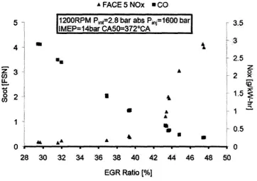
Besides the direct effect on NOx emission and temperature control of the engine, the EGR

below 0.5 g/kW-hr, soot increases significantly with a high rate of increase. This means a

little EGR ratio increase will result in high soot emission.

*FACE5NOx «CO

z 3

a.

o

o n

to c

] i

j m

I ^ U U K K M Kiri,=z.o Dar aDS rjnj=

|IMEP=14bar CA50=372°CA i % |

•

At A * A ""

=iom

4

A A

0 j o a r i

A •

I

i

- 4 o

EGR Ratio [%]

Fig. 1.1 EGR Sweep SootNOx

The portion of exhaust gas re-circulated back into intake manifolds is controlled through

to the open position of an EGR valve. So, an accurate and fast EGR valve control is

necessary to meet modern emission standards.

1.2 Current Control Methods

Different approaches have been proposed to address the control of the valves in general.

In [11-14] the methods to control the EGR valve are detailed. Usual implementations are

based on PID algorithm. In [32] the control strategy based on neural networks is

discussed. A discrete-time implementation of a variable structure controller with sliding

proposed in [34]. In [35] two simplified different sliding mode controllers based on a

simplified second order plant model are presented.

However, these control methods which are currently in use, such as PID or sliding mode

controller, take an enormous effort to find the optimized parameters for the controllers,

and in many cases they cannot provide sufficient control accuracy on the valve position.

In fact, in most cases, the designed system could not meet the required performances.

1.3 Proposed Control Method

The throttle valves are usually controlled in one direction, opening direction, using

unidirectional drivers and closed automatically with the spring force. In advanced control

techniques, the throttle valve is controlled in both opening and closing directions using a

bidirectional driver. So, with an appropriate control method and using a bidirectional

driver the valve could be precisely controlled in both closing and opening direction. Here

the Model Predictive Control method is proposed to control the valve.

Model predictive control method does not yield the optimal solution for the control

problem but with a good approximation at each instant calculates the control inputs using

the receding horizon concept. In fact the purpose of this method is to drive the future

outputs of the system close to the defined reference trajectory.

1.4 Estimation of Spring Torque

satisfied [25-27]. Specifically, low temperature combustion is a hopeful mode that would

facilitate low NOx emission while still keeping the engine efficiency high [25]. An

important fact in such a mode is that the feasible combustion window is very narrow. This

in general requires faster transient responses from controlling valves and, hence, calls for

advanced control of valve operation that could allow faster and accurate performance. In

the EGR valve case, the accuracy requirement for the valve plate position (opening or

closing) would be more stringent and the control must be more prompting in order to

facilitate low temperature combustion

The total torque acting on the valve plate is actually the sum of the motor torque and a

spring torque which goes against the plate during opening session and serves as an extra

assisting torque during the closing session. Since this spring torque is not regulated by the

motor drive controller, for faster and more accurate control of such a throttle valve it is

important to estimate the spring torque so that the information could be used to further

improve the motor torque control. Here, the spring torque is treated as a disturbance

torque and model based robust estimations are developed using the ideas in [22-24] to

estimate this torque in a throttle valve.

The disturbance torque estimation for a DC motor is reviewed in many literatures. In

[21-23], estimation of disturbance torque on the DC motor shaft has been proposed and

developed. In [21] the disturbance torque acting on the motor shaft is assumed to be

constant with respect to the dynamics of the filter and a Luenberger filter is proposed

[21]. In [22-23], the disturbance torque is treated as an uncertain variable input and a

estimation of the disturbance torque could be calculated from the current and speed

estimation.

Hence, to have a faster and more accurate control of the throttles valve which is a

necessary in advanced control engine, the spring torque is treated as a disturbance torque

applied to the motor shaft and three filter designs, namely, Kalman, H^, and, H^

Gaussian, are developed and compared to estimate the spring torque

1.5 Thesis Outline

This thesis is arranged as follow: in Chapter 2 the preliminary theory of Model Predictive

Control method and Generalized Predictive Control algorithm is detailed. The theory

required for the observer design and different methods to calculate the observer gain are

developed.

In Chapter 3 Hardware-in-Loop (HIL) setup configuration and tests done to evaluate the

effectiveness of proposed control algorithm for the EGR valve are detailed, and the

configuration and method to obtain the spring torque is presented.

In Chapter 4 the model of the EGR valve is derived. The model parameters are identified

while the identification methods are discussed and the accuracy of the parameters are

validated.

In Chapter 5 based on the model of the system and the parameters identified in Chapter 4,

the GPC algorithm for the EGR valve is derived, the future output of the plant and the

In Chapter 6 using the model obtained in Chapter 4, the methodology to design the spring

torque observer for the EGR valve which includes the state space models of observers is

detailed. The experimental validations for the estimated torque are shown.

Finally the thesis is concluded in Chapter 7 and recommendations are made for future

CHAPTER 2

PRELIMINARY THEORY

2.1 Model Predictive Control (MPC)

Model Predictive Control method (MPC) refers to a wide range of control methods which

uses the model of the system to minimize a cost function and consequently to calculate

the control signal [15]. This wide range of MPC methods is only different in the defined

system model, the cost function and the noises [15]. In this method a sequence of future

outputs is predicted using the process model, while the control sequence is calculated by

minimizing an objective function [15]. This objective function is defined in terms of

system error between the predicted output and reference trajectory [15]. The advantage of

this method is to the use of predictive inputs sequence which would allow a faster control

on the system. For this purpose to reflect the full dynamics of the system, it is necessary

to model the plant in the best possible way.

The methodology of all the controllers belong to MPC family is represented in [15]. This

method applies a dynamic model of the plant to generate a set of predicted outputs

y(t + j\t) in a finite horizon, N sampling time, by using the known input and output values

up to the present time. At the same time the criteria function, usually defined in terms of

error signal between the predicted output and the defined reference trajectory, is

minimized during the process and the set of future control signals is calculated. Since at

of the control sequence, the signal corresponding to the time t , is sent to the system and

the new data is used to calculate the next control signal u(t +1|? +1).

MPC controller

cost function

• • : ! + •;'.

constraints

• • —

X

u

' r

Plant

state estimator

y

Fig. 2.1. MPC control loop

The basic structure to implement the MPC strategy is shown in Fig. 2.1. As can be seen,

using the plant model the future output of the system is predicted based on the past input

and output of the system and the optimized future outputs. These predicted output are

compared with the defined reference trajectory, and the error comes from the difference

of these two signals is minimized and used to calculate the next control input by the

optimizer [15-17].

Therefore, this approach provides a forward prediction in the control and hence can

potentially provide a faster response while the accuracy can be improved during the

operating process in the long-run.

1. Predictive Model

2. Objective Function

3. Obtaining the control law

According to the different options which can be used for each of these elements the

proposed algorithm may vary [15].

1. Predictive Model

Since this method is a model based method, the process model plays a critical role in the

controller. The plant model should be able to fully capture the system dynamics, while it

should be simple enough to implement, and allow the prediction of the future outputs to

be calculated and analyzed [15]. Various types of models are used in different MPC

formulations. Impulse response, step response, state space, transfer function and nonlinear

models are different methods which could be used in the MPC formulation according to

the chosen method. Selection of disturbances model, the difference between the measured

output and the one calculated by the model, is also as critical as choosing an appropriate

process model [15].

2. Objective Function

Various MPC algorithms may use different objective functions to calculate the control

law. The purpose of defining this criterion is that the predicted output follows a defined

reference trajectory, minimizing the future error, on a finite control horizon, while the

future control signals applied to the system are calculated. The most common expression

for this function takes the quadratic form of the errors between the predicted future

3. Obtaining the Control Law

The control signal sent to the system is calculated by minimizing the objective function

on a finite control horizon. So this signal is a function of the past inputs and outputs of the

system which are known at the present sampling time and the predicted future outputs and

the reference trajectory defined for the system.

2.2 Generalized Predictive Control Algorithm

Generalized Predictive Control (GPC) is one of the most popular Model Predictive

Control (MPC) methods proposed by Clarke al. [16-17]. This method is capable of

controlling a wide range of plants with variable design parameters and variable

dead-time, and even unstable and non-minimum phase plant [15-17]. It is a proven successful

control strategy for industrial application as long as the sampling period implemented is

long enough to carry out the calculation [18]. This control method has been used in

applications such as autopilot design [18], brushless DC drives [19], and direct drives

[20].

GPC method is based on the same concept as MPC and has many ideas in common with

the other predictive controllers, but it has some differences as well [15]. This method can

deal with unstable and non-minimum phase plant and incorporates the concept of control

horizon as well as the consideration of weighting of control increments in the cost

A single-input-single-output (SISO) plan, when linearized and regulated around a

particular set point can be modeled by a Controller Controlled Auto-Regressive and

Integrated Moving Average (CARIMA) model [15-17]:

A{z-X)y{t) = B(z-X)u{t ~ 1) + C ( Z y ( 0 (2-1)

A

Where u(t) and y(t) are the control and output sequence of the system, C,(t) is the zero

mean white noise, and A is the differencing operator 1 - z"1. A, B and Care polynomials

in the backward shift operator z~x:

A{z~l) = 1 + axz~x + a2z~2 + ... + anaz~na

B(z~l) = b0+blz~1 + b2z~2+... + bnbz"nb (2.2)

C{zTx) = 1 + cxz~x + c2z~2 +... + cncz~"c

For simplicity, the C polynomial is chosen to be 1 or C"1 is truncated and absorbed into A

and B [15-17].

The GPC controller specifications are formally described using the following cost

function [15]:

J{N

N

,N

)= ^SUlW + jfi-Mt + fif + Zmitoit + j-l)]

(2.3)

Where JV,, N2 are the minimum and maximum costing horizons, Nu is the control

horizon. In the systems with unknown dead-time Nl can be to 1 with no lost of stability,

and in discrete time event JV2 should exceed the degree of5(z_1). Nu is an important

value of Nu could increase till it reaches the stage that any further increase in this

parameter makes very little difference [15-17]. S(J), and A,(j) are the weighting factors

of the predicted error and the control effort during the optimization [15-17]. In the above

equation, in the most cases a reference trajectory w(t + j) is used which does not

necessarily have to coincide with the real reference. It is usually a first order

approximation of the current output values towards the known reference [15]

w(t) = y(t) w(t + k) = aw(t + k-Y) + (l-a)r(t + k) * = 1.JV (2.4)

Where a is a parameter between 0 and 1. By choosing a small value of or a fast tracking

of the reference is provided while increasing this parameter yields a smooth reference

tracking.

The next Diophantine equation is used to calculate the future output sequence:

l = £ / z -1) i ( z -,) + z ^ . ( z -1) (2.5)

Where: A(z~l) = l-A(z~l)

The Ej and F. polynomials can be obtained by dividing 1 over the A(z~^) to the point

that the remainder can be factorized as z~JFj(z~l) [15-17].

If the multiplication of the CARIMA equation with AEj(z~i)zjis substituted into the

Diophantine equation the jth step ahead sequence of the output plant can be obtained.

After the mathematical calculation the future output of the plant can be obtained by:

Where:

y =

y(t + l\t)

y(t + N\t)

u =

Au(t)

Au(t +1)

Au(t + N)

G(z-x) = E(z-x)B(z-x)

go

gi

0

So

0 0

gN-l gN-2 '" g(i

F(z~x) = F 2{z~x)

FN(z-X)

G\z~x) =

(Gd+i(z )~go)z

(Gd+ii^-go-gi^V

(Gd+3 (z"1) - g0 - glz-1 - - gN_^N-» )zN

The last two terms of the above equation clarify the past information of the plant and can

be grouped as / .

Therefore, the future output equation can be written as:

y = Gu + f (2.7)

Finally, the future control input can be obtained by minimizing the cost function over the

control horizon. By considering the two weighting factors A, and 5 in minimization the

control input is calculated. Equation (2.3) can be written as:

J = 8x(Gu + f -wf(Gu + f -w) + AuTu

After simplification, the objective function is written as:

J = - uTHu + bTu + f0 (2.9)

where:

H = 2(SGTG + AI)

bT =2S(f-w)TG (2.10)

f

= S(f~w)

(f-w)

By making the gradient of J equal to zero, the minimum of J is obtained:

u = -H-lb = (SGTG + AiylSGT(w-f) (2.11)

The control signal sent to the plant is the first element of the vector u which is given by:

Au(t) = K(w-f) (2.12)

Where K is the first row of matrix (SG1G + AI)~X dGT and w is the defined reference

trajectory.

2.3 Filter (Observer) Design

For an ideal system where no disturbance and model uncertainty is considered on the

system, the Luenberger filter is used as the simplest filter design. In fact, Luenberger

filter is designed for an ideal system, and its performance in the real world is usually not

spring torque as an external disturbance torque while considering the model uncertainty

and disturbances on the system.

• Kalman Filter

Kalman filter is used to estimate the state variables for the system subjected to the white

noise. This filter estimates the state variables in a noisy environment by minimizing the

variance of the estimation error.

For Kalman filter design, the state space model of the valve system is modified by

including noises in:

x = Ax + Bu + ^

z = Cxx (2.13)

y = C2x + 0

Here x is the state variable, u is system input, y is the measured output, z is the desired

output, A and B depend on the model parameters.

In the state space model of Kalman filter,^ and9are the noise inside the valve system

and in the measurement respectively. It is assumed that the average values of both the

noises, ^ and 6, are zero and there is no correlation between them. These two noises are

modeled by a white noise w0 with power spectrums: £" = Bowoand0 = D20w0. In practice,

B0 and D20 are set by measuring the covariance of the measurment noise and process

noise respectively.

{A-BA^CJP + PiA-BtDl^Cj+B^I-Dl^D^Bl

T 1 ( 2-1 4 )

So:

Lk^-(B0D^+PC2)P^1 (2.15)

where: BQ = D20Dl0

• H^ Filter

When the system model parameters are uncertain and bound to change with time or

process, these uncertainty should be taken into account when the state variables are

estimated. For such a system, Hx filter is designed to make the state estimation robust to

changes in model parameters.

x - Ax + Bu + Bxw

z = Cxx (2.16)

y = C2x

Bx is the weight given to the uncertainty disturbances, w, depending on its effect on the

system performance.

The Hx filter gain is obtained by solving the Riccati equation [31]:

AP + PAT + P{y~2CxTCx - C2TC2 )P + B^B? = 0 (2.17)

So:

Here y is the design parameter which decides the limit of uncertainty which could be

tolerated by the filter for good performance. Lower the value of y , higher the tolerance

of the filter towards to model uncertainty.

• H^ Gaussian Filter

A practical system is subjected to both white noise and parameter uncertainty. The

Kalman filter is designed to achieve good performance against white noises while it is

model dependant and sensitive to parameters variations. The Hx filter is designed to

handle model parameters variation; however it does not to give good performance against

white noise. So the performance of these two filters conflict each other. So for the case

when the system is subjected to both model parameters uncertainty and white noise, Hn

Gaussian filter is designed based on constrained optimization result and Hx optimization

design. This filter is designed using a parameter y which decides the weight which gives

the weight that is given to the performance of each type of the filters, thus obtains a

suitable balance between the performances of the two filters.

The system model that accommodates the Hx Gaussian filter is design by considering

both white noises and model parameters uncertainty:

x = Ax + Bu + BQWQ + Bxw,

z = Cxx, (2.19)

y = C2x + D20w0,

For the Hx Gaussian filter design, the filter gain is obtained through solving two Riccati

equations [29]:

(A -P2C2TR^lC2 -B0D^C2)TPX +Pl(A-P2CWC2

-B0D^lC2) + r~2PAB[Px + C f c = 0

( ^ - V U - ^ + r ^ ^ +P2(A-BQDT2^xC2+y-1BlRlPl)T

-P2CT2K^XC2P2 +B0(I-D^D2Q)B^ = 0

(2.21)

So the gain value is calculated as:

CHAPTER 3

Hardware Setup

3.1 Hardware-in-Loop Configuration

Hardware-in-Loop (HIL) testing is used to check the performance of a system design

subject to real world loads and disturbances. In HIL simulation, only the designed system

is composed of hardware parts, the remaining plant dynamics are provided by software.

This testing helps in obtaining the required data before implementing the designed model

in an actual system thus saving cost and time taken to test the efficiency of the design. It

is also suitable in cases where testing the design in the entire system is not feasible due to

physical constraints and safety reasons. The HIL setup to test the EGR valve control loop

is shown in Fig. 3.1 and the setup to estimate the spring torque is shown in Fig. 3.2.

Power Supply

Torque

Dynamometer Sensor Valve

Fig. 3.2 Hardware setup to estimate the spring torque

In the hardware setup to control the EGR valve, Fig. 3.1, the GPC controller is

implemented by a TMS320LF2407 DSP with 40MHz CPU clock. The reference voltage

from the Opal-RT output terminal and the feedback voltage which in fact shows the plate

angular position are the analog inputs of the DSP. The feedback voltage varies between

around 1.4F for the fully close condition to 3.2V for the case when the valve is

completely open. After applying the GPC algorithm, the output of the DSP is applied to a

bidirectional driver in form of a PWM wave. This driver applies the control input as a

voltage across the motor armature.

The experiment setup to measure the spring torque is shown in Fig. 3.2. As can be seen,

the valve is connected to a dynamometer through a torque sensor. The torque sensor

measures the effective torque acting on its shaft. In the experiment, the dynamometer

produces a torque of 0.5 Km applied to one end of the torque sensor shaft, on the other

the total torque on its shaft including the spring torque, it is impossible to obtain the

spring torque through direct measurement. Therefore, an indirect way is conducted by

performing two sets of experiments in order to calculate the spring torque. In the first

experiment the spring is connected between the motor and the plate shaft. In this case the

total torque acting on the torque sensor shaft is Tls-T^,no+T —Ts, where Tts is the

torque measured by the torque sensor, Td is the dynamometer torque, T and Ts are the

plate (hence the valve motor) and the spring torque respectively. In the second experiment

the spring is taken off so the torque measured by the torque sensor is Tts = T, + T .

Clearly, the difference in the two readings of the torque sensor would be the spring

torque. During the experiments, the filter estimation is executed at the same real time as

the real experiment to keep the integrity of the transient process. The experiment is done

by applying voltage of 6 V to the valve when the spring is disconnected and 4 V to it when

there is the spring connected there. These two voltages produce the same current and as a

result the same motor torque. However, in the first case the valve opens completely and in

the second case it opens only half way. Then the real valve operation (opening) and the

filter estimation are conducted at the same time.

3.2 Hardware-in-Loop Equipment

• DSP TMS320LF2407

The TMS320LF240x devises are part of the TMS320C2000 plat form of fixed-point

DSPs. The 240x devices offer the enhanced TMS320DSP architectural design of the

Highly developed peripherals, optimized for digital motor and motion control

applications, have been integrated to provide a single-chip DSP controller.

The 240x offers increased processing performance, 30M instruction per second, and a

higher level of peripheral integration. It offers up 32K words of on chip Flash devises

contain of 256-word boot ROM to facilitate in-circuit programming. It offers two event

manager optimized for digital motor controller and power conversion applications. These

two modules have the capability of controlling multiple motors and/or converters,

generating symmetric and asymmetric PWM outputs, programmable dead band, and

synchronized analog-digital conversion.

The following DSP peripherals are used in the EGR valve control development:

1. Analog to Digital (ADC) Converter Module

The ADC module consists of a 10-bit ADC with a built-in sample-and-hold (S/H) circuit.

The high-performance, 10-bit analog-to-digital converter has a minimum conversion time

of 500 ns. For these converters a maximum of 16 conversions is allowed to take place in a

single conversion session without any CPU overhead.

2. Event-Manager Modules

The event-manager modules include general-purpose (GP) timers, full-compare/PWM

units, and capture units. Only one of the two general-purpose timers is used to generate

the desired PWM signal. This timer includes a 16-bit timer, up-/down-counter, TxCNT, a

bit timer-compare register, TxCMPR, a bit timer-period register, TxPR, and a

16-bit timer-control register, TxCON. The period register shows the full period of the PWM

The TMS320LF2407 evaluation module is used to apply the certain characteristics of the

LF2407 DSP. Fig. 3.3 shows the basic configuration for LF2407 EVM and its features.

K

K=

c

LEDs

K

CAN DRIVER

K

/-3

S>

3

DATA ANALOG

K

ADDRESS

TMS320LF2407

CONTROL

PWWIO

SPI JTAG DART

7)

^C

/ \ A

\y

f¥

K

JTAGP5

LOGGING ' INTERFACE;

Fig. 3.3 Block diagram of TMS320LF2407 EVM

A

-/

Two of 16 channels of analog to digital converter are used to convert the analog reference

signal comes from the Opal-RT, and the system feedback comes from the position sensor

to digital values. Using these two digital values the GPC control algorithm is

implemented, and the control value is calculated. Since the control signal applied to the

driver should be a PWM wave, this value is used to generate a PWM signal. The board is

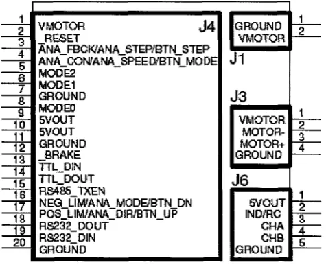
• Motor Driver Configuration

A PWM controlled driver board is used for bi-directional control of the DC motor

connected to the EGR valve. The control signal from the DSP is applied to the driver

control pins, J4 in Fig. 3.4, and the equivalent voltage is applied to the valve motor

through pins 2 and 3 of J3. All connectors of the motor driver used in this development

are shown in Fig. 3.4.

1 2 3 4 5 e 7 8 9 10 11 12 13 14 15 16 17 18 19 20

VMOTOR J 4 RESET

ANA FBCK/ANA STEP/BTN STEP ANA CON/ANA SPEED/BTN MODE MODE2 MODE1 GROUND MODE0 5VOUT 5VOUT GROUND BRAKE TTL DIN TTL DOUT RS4fl5 TXEN

NEG LIWANA MODE/BTN DN POS LIM/ANA OIR/BTN UP RS232 DOUT RS232 DIN GROUND GROUND VMOTOR J1 J3 VMOTOR MOTOR-MOTOR+ GROUND J6 5VOUT IND/RC GHA GHB GROUND 1 2 1 2 3 4 1 2 3 4 5

Fig. 3.4 Motion Mind driver

There are different operating modes for the driver. Here the bi-directional analog mode is

used to control the valve in both directions. In this mode the 0-5 V signal present at

ANASPEED (J4 P4) is translated into the motor speed while a dead-band centered at

2.5 V exists (2A3V-2.57V). If the analog input falls within this range then the motor is

stopped. The relationship between the analog input to the driver board and its output is:

where Vjn is the control signal sent by the DSP and Vout is the voltage applied to the motor.

• Dynamometer

A 5hp, 3 phase, 240 V, 22Amp Baldor induction motor is used as the dynamometer. This

dynamometer produces a torque of 0.5 N.m on the torque sensor shaft. The maximum

torque the motor can produce is 20.18 N.m and the minimum torque is 0.1 N.m.

• Dynamometer Controller Configuration

A vector drive is used to control the torque of the dynamometer. The configuration used

by the dynamometer is as follow:

Operating Mode: Bipolar, Open loop vector mode

Operating zone: Quiet variable torque, 8kHz PWM

Command source: Analog Input 2

Analog Input 1: Current limit source, 0 to \QV

Analog Input 2: Torque signal, -lOFto 10F

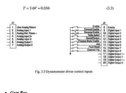
The drive control is operated by the opto-isolated digital inputs J2-8 to J2-20 shown in

Fig. 3.5. The opto inputs can be switches or logic signals. In this case transistors were

used to switch the inputs on and off, as they can be controlled by analog signal from

Opal-RT.

The torque produced by the dynamometer is controlled by Analog Input 2 and the

direction is controlled by the digital switches FWD and REV. For a positive torque, a +ve

a -ve signal is sent through Analog 2 and the REV direction is selected. The relationship

between the control signal, V sent to the dynamometer and the torque, T (in Nm) is:

r = 3.6F + 0.036 (3.2)

J1 1 2 3 4 5 6 7

User Analog Return Analog Input 1 Analog Ref. Power + Analog Input 2+ Analog Input 2-Anatog Output 1 Analog Output 2

Enable Forward Enable Reverse Enable Table Select Speed/Torque

Y-o^h-Process Mode Enable

Jog Fault Reset External Trip

J2

Fig. 3.5 Dynamometer driver control inputs

8 9 10 11 12 13 14 15 16 17 18 19 20 Enable Digital Input 1 Digital Input 2 Digital Input 3 Digital Input 4 Digital Input 5 Digital Input 6 Digital Input 7 Digital Input 8 Digital Output 1 + Digital Output 1 -Digital Output 1 + Digital Output 2

-• Gear Box

Since it is expected that the spring torque be estimated as a very small value, a gearbox is

used to amplify the valve (DC motor) torque. The ratio of the gear box is 1:20 which

means the valve torque is magnified 20 times. The gearbox is designed such that the

torque flow is permitted in only one direction from the high speed (low torque-input) side

to low speed (high torque-output) side. This design is for safety reasons to ensure that the

• Torque Sensor

A torque sensor is used to validate the estimation result of the spring torque. The torque

sensor operated as any other strain gage sensor. When the motor is operated with no load

torque acting on the gear box shaft, dynamometer in off condition, the output of the

sensor is zero as there is no torsion force on the torque sensor shaft. When the

dynamometer is in on condition, the torque sensor shows sum of the total torque acting on

its shaft.

• Opal-RT Configuration

The Opal-RT is configured to run a 1ms step size and the data is stored by using the

Op-write data logging block. Opal-RT is used in both the development to control the EGR

valve and to estimate the spring torque. In the first development, since the control

algorithm is implemented by the DSP the Opal-RT is only used to apply the reference

signal, plot and store the control results. In the second development, the Opal-RT is used

to get the current and voltage samples of the system and run the observer model at the

CHAPTER 4

Modeling EGR Valve

4.1 Modeling of EGR Valve

The electric throttle valve modeled in this study is a two plate butterfly valve driven with

a low power DC motor. The DC motor mounted on top of the plate body is connected to

the plate shaft through the gears. So the motor torque is magnified through these gears

when applied on the plate shaft. The other side of the plate shaft is connected to a position

sensor. This sensor is in fact a potentiometer converts the plate angular position into a DC

voltage used for the plate position control. This output voltage varies in the range from

1.4 Vto 3.2 V. The voltage 1.4 Vshows the valve fully close position and 3.2 Vshows the

fully open position of the EGR valve.

Also there is a spring connects the plate shaft to the motor shaft. This spring adds an extra

torque to the plate which helps the valve in closing direction and acts against it in opening

movement. In Fig. 4.1 the EGR valve modeled in this study and the motor gearing part to

Position

Sensor Motor

I

I

Motor shaft is geared

to the plate shaft

Fig. 4.1 The EGR valve and motor gearing to the plate shaft

^m->"m

i

Fig. 4.2 The schematic diagram of the EGR valve

In order to model the EGR valve, first the DC motor which drives the valve is modeled,

additional torque added on the motor shaft. So the full model of the valve could be

derived.

The armature controlled DC motor provides the motor torque to drive the plates. It is

noted that the motor torque is amplified through the gearbox before applying the plate

shaft. The following equations can be established to model the motor drive.

V = RJa+La-jj^ + ea (4.1)

ea=Ke6m (4.2)

Tm=Ktia (4.3)

Tm-Tf=jJm+Djm (4.4)

The electrical model of the motor is shown in equation (4.1) where Ra and £aare

resistance and inductance of the motor armature winding, ia is the armature current, and

ea is the internally generated voltage which is proportional to the motor velocity. 6m is

the motor angular position. Ke and Kt are the voltage and torque constants which in SI

units have the same value. In equation (4.4) the motor dynamic parameters, inertia and

viscous damping factor, are denoted as Jm and Bm, while Tj is the friction torque on the

motor.

The torque equation for the whole EGR system is shown in the following equation:

Tp=J0p+Wp+nks0p (4.5)

Where J and B are the total moment of inertia and viscous damping factor of the system

in which both motor and plate dynamic parameters are considered, n is the gear ratio and

nkfi presents the stiffness of the spring which is actually ignored in the control design.

With equations (4.1) to (4.5), the electric throttle valve can be modeled in single shaft as

follow:

V = Raia+La^ + Ken6p

Tm = Ktla

Tp=JOp+D0p

(4.6)

(4.7)

(4.8)

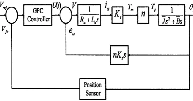
The model derived above can be presented using Laplace transfer function in the block

diagram shown in Fig. 4.3:

'+i

Y.

J

'ea

1

^«+V

la

— »

K,

T

m

»

M T^ C

1

l^t°

n

1

Js

+Bs

8

Fig. 4.3 The block diagram of EGR valve

In this block diagram Tm is the motor torque produced by the armature current. This

torque after magnifying through gears drives the valve. The plate position is the output of

The state space model of the EGR system can be derived by considering armature current,

plate angular position and plate angular speed as three states of the plant:

x = Ax + Bu y = Cx

x-r _

xx

Xj

3.

=

-la

°

P

K.

u = V

(4.9)

y=o

Using the system model the A, B and C are derived as:

A = -R

nL„

0 0 1

& 0 I

J J

B = 0 0

C = [0 1 0]

In order to complete the model of the EGR valve the system parameters such as Ra, La,

J , B, Kt should be identified. Since the system parameters for this development are not

available, it is required to determine these values experimentally to obtain the complete

EGR valve model. In order to determine the motor parameters Ra, La and Kt the

experiments are conducted on the motor itself when it is disconnected from the plate.

Two mechanical parameters J and B are obtained through the experiments on the whole

1. Armature Resistance

A very small voltage, Vt, is applied to the motor terminals, the rotor is blocked for few

seconds. Using a very small resistance, rshmt, the current, ia, is read quickly when it

reaches the steady state. Since the rotor may heat up slightly it should not be blocked for a

long time. The armature resistance can be calculated as:

Ra = Vt~rshuntla ( 4 1 0 )

shunt

Since the armature resistance highly depends on the shaft position, the experiment is

conducted several times on the motor and the final value is obtained by taking the average

of the calculated values.

2. Armature Inductance

The armature inductance, La, could be calculated by measuring the phase lag between the

motor low amplitude voltage and current when the motor rotor is blocked. Since the result

of this experiment is too noisy in this case, the motor inductance is simply measured by

using an inductance meter.

3. Electrical and Mechanical Constants

In a DC motor considering the SI units the electrical constant, Kv (V/rad/s) is equal to the

mechanical constant, Kt (Nm/A). In this case the motor internally generated voltage is

measured and used to calculate these two constants. For this experiment the valve is

constants are calculated by measuring the voltage internally generated across the motor

terminals, motor speed and the gear ratio.

So the motor constants are measured as follow:

Kv=Kt=— (4.11)

<nm

where v is the motor internally generated voltage, a>m is the motor speed in RPM.

4. System Viscous Damping Factor and Inertia

Since the system is modeled using the total viscous damping factor and total inertia, these

two parameters are calculated by conducting couple of experiments on the whole valve.

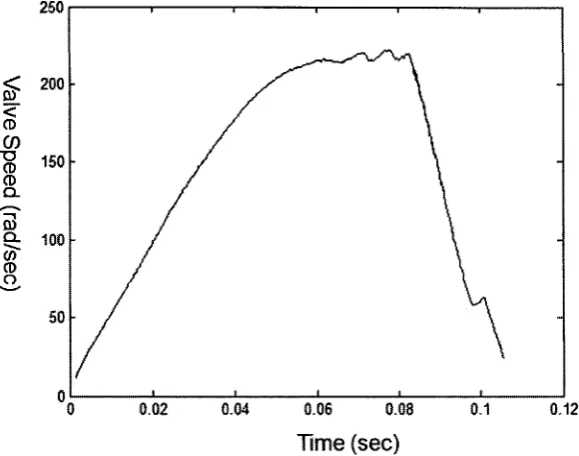
In order to find system moment of inertia and viscous damping factor, 8 different step

voltages in the range of 2-10V are applied to the EGR valve and the corresponding speed

and current responses are analyzed. Fig. 4.4 shows the speed response of the system when

a voltage of 10 V is applied to the system. The acceleration period is divided into 6 small

periods; the system acceleration, speed and current are measured in these small periods

and used to calculate the system inertia and damping factor.

Zal

*a2

*a3

*a4

la5

Ja6j

=

Jx

a\ a2

a3

a4

a5 .a6_

+ B cox 0)2

0)3

(04

(D5

Using the above equation, two mechanical parameters of the system are calculated.

0.06 0.08

Time (sec)

Fig. 4.4 Plate speed response for the applied 10 V

0.12

As can be seen in the Fig. 4.4 after 0.08 seconds the system speed drops suddenly to zero,

which shows the valve is blocked at this time. This is also observable from the current

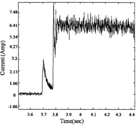
response of the system when the same voltage of 10 Fis applied to the system, Fig. 4.5.

As can be seen, immediately after the current reaches the steady state value of 1.06Amp,

there is a sudden jump to 7.4 Amp, and then it reaches another steady condition. The

reason for this jump is that after almost 0.08 seconds the plates reach the block, the EGR

valve in this experiment can only open 90°, cannot go further. So, only the data within the

7.48-6.41

5.34 4.27

O 2.13

1.06

0

-1.06

kw*<Nw

i t i i i i i

J i i_

3.6 3.7 3.8 3.9 4 4.1 4.2 4 3 4.4

Time(sec)

Fig. 4.5 Plate current response for the applied 10 V

Each experiment is repeated 2-3 times and the average taken to get more accurate values.

4.2 Validation of Model Parameters

Through more investigation by evaluating the identified parameters with a Simulink

model, it was found that the system viscous damping factor identified through

experimentation, slightly changes when the applied voltage varies between 0 to 10 V. This

slight difference can be due to the nonlinearity of the system. So in the open loop

experiment, the full operating range is treated as a series of narrow operating range

problems and 2 different linear models, each valid for a range of operation, is developed.

uncertainty is compensated and only the first set of parameters is accurate enough to show

the system model.

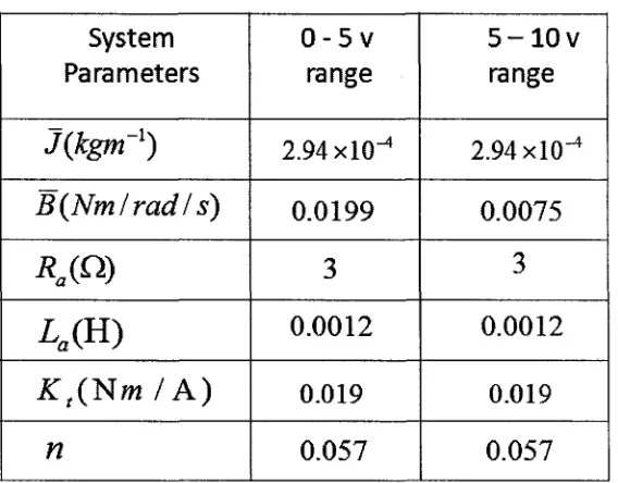
Table 4.1 shows the identified parameters for two operating ranges:

Table 4.1. EGR valve identified parameters

System Parameters

Jikgm'

)

B{Nmlradls)

R

{&)

4(H)

^(Nm/A)

n

0 - 5 v range

2.94x10^

0.0199

3

0.0012

0.019

0.057

5 - l O v range

2.94 xlO-4

0.0075

3

0.0012

0.019

0.057

The model obtained in this section is used in both control algorithm and in observers

CHAPTER 5

Control Design for EGR Valve and Experimental

Validation

5.1 GPC Algorithm for Control of the EGR Valve

In order to control the EGR valve using the GPC algorithm, the input and output of the

system are allowed to be U{t) and 0 ( 0 . In the close loop system when there is a

feedback in the system, the uncertainty in the viscous damping factor of the valve is

compensated. So only the first set of model parameters identified in Chapter 4 is accurate

enough to use in the GPC algorithm.

Since in the GPC method the transfer function of the system is used, the EGR valve is

modeled as:

u(t) U(t) 3.5282 x 1 0_V + 9.0594 x l O ~ V + 0.16835

A and B polynomials in equation (2.1) can be obtained when the transfer function of the

system is transferred to the Z domain:

A(z~x) = 1 - 1 . 9 l z- 1 + 0.988z-2 - 0.0767 l z- 3

5(z"1) = 2.48xl0"5+1.818xl0~4z"1+1.119xl0~4z"2+5.414xl0~6z"3

Via applying equationA(z~l) = AA(z~1), the plant model is used to obtain the A(z~l)

A(z-y) = AA(z~l) = l - 2 . 9 1 z_ 1 + 2.898z-2 -1.0647z- 3 + 0.07671Z-4

In order to calculate the future outputs of the plant, the two Controller Auto Regressive

Integrated Moving Average and Diophantine equations are used. When ^(z_1)is

calculated the E and F- polynomials in equation (2.5) for a 4 control horizon are

obtained by dividing 1 over the A(z~l) to the point that the remainder can be factorized

as z~JF(z~l). So theses polynomials are calculated as:

£1=1

E2= 1 + 2.9 lz_ 1

£3= l + 2.91z_1 +5.570 \z~2s

£4= l + 2.91z_1 +5.570 lz_ 2+8.8405z- 3

Fx = 2.91 - 2.898z_1 +1.0647z"2-0.07671z"3

F2 = 5.5701-7.3685z_1 +3.0216z- 2 -0.2232z- 3

F3 = 8.8405-13.1205z_1 + 5.7073z~2 -0.4273z- 3

F4 = 12.6054 -19.9125Z"1 +8.9852z"2 -0.6782z- 3

The future output of the plant is calculated using the following equation:

Notice that the last two terms in equation (5.2) only depend on the past and can be

grouped into f leading to:

y =

Gu

+ f

where:

y =

y(t + \\t)

y(t + 2\t)

y(t + 4\t)

G(z-1) = E(z~1)B(z-1) =

' 2.495 xlO- 5

2.5725 xlO- 5

7.9566 xlO- 4

1.5xl0"3

1/ —

ft —

Au(t)

Au(t +1)

Au(t + 2)

Au(t + 3)

0 0

2.495 xl(T5 0

2.5725 xl(T5 2.495 xlO- 5

7.9566x10 ~* 2.5725 xlO- 5

0

0

0

2.495x10

/ =

1 . 8 4 x l 0 "4A ^ - l ) + 1 . 1 4 x l 0 ~4A ^ - 2 ) + 5.541xl0"6Aw(r-3)

+2.936y(t) - 2.95 \y{t - 1 ) + 1 . 0 9 3 9 ^ - 2) - 0 . 0 7 8 9 1 ^ - 3)

6.5422 x 10- 4 Au(t -1) + 3.4024 x lO~4Au(t- 2) + 1.6268 xlO~5Au(t- 3)

+5.669ly(t)-7.5702y(t-l) + 3A328y(t-2)-0.2317y(t-3)

1.3xl0~3Aw(f-l) + 6.6255xl0"4Aw(f-2) + 3.1412xl0~5Aw(?-3)

+9.0743^(0 -13.5967 y(t - 1 ) + 5.9697 y(t - 2) - 0 . 4 4 7 3 ^ - 3)

2.4xl0~3Au(r-l) + 1.03xl0~3Att(/-2) + 5.0281xl0~5Aw(*-3)

Now that the future outputs of the plant are obtained, the objective function J can be

calculated:

J = —uTHu + bTu + f0s (5.4)

where:

H = 2(SGTG + ZI)

bT =2S(f-wfG

f0 = S(f-w)T(f-w)

By making the gradient of J equal to zero, the minimum of J is obtained:

u = -H~lb = (SGTG + Aiy1SGT(w-f) (5.5)

The control signal sent to the plant is the first element of the vector u which is given by:

Au(t) = K(w-f) (5.6)

Where K is the first row of matrix (SGT G + AT)'1 SGT and w is the defined reference

trajectory.

It is observed that the set of weights A,(j) = IxlO~ and S(j) = 35gives the best

performance.

The reference trajectory is defined as a smooth approximation from the current value of

the output towards the known reference by means of the first order system:

a is a parameter between 0 and 1. This parameter is chosen as 0.3 in this case to give a

smoother approximation of the real reference.

After all the calculations the matrix K and the control input of the EGR valve is

calculated as:

^ = [88.2 725.8 938.3 -22.5]

A«(0 = 88.2w(7 +1) + 725.8w(7 + 2) + 938.3w(f + 3) - 22.5w(t + 4)

- 1 JQ7SAu(t - 1 ) - O.S26SAu(t - 2) - 0.0392Au(t - 3)

- 1 . 2 5 9 4 x l o V ( 0 + l - 8 0 4 4 x l 04^ - l ) - 7 . 7 5 8 4 x l 03j ; ( r - 2 ) + 5 7 8 . 7 1 7 1 ^ - 3 )

(5.8)

The final block diagram of the EGR valve controlled by the GPC controller is shown in

Fig. 5.1:

T>

h

GPC Controller

Wrf

T

1

Rtt+Las

ea

Position Sensor

I.—, f .—.T

a T. Am r

_K

— ,

_

- nK

s

1 «4

J$2+Bs

Fig. 5.1 The block diagram of the EGR valve controlled by GPC

The input of the system is a voltage applied from the Opal-RT output. The GPC controller

the system error. Plate position is the output of the system which converts to a DC voltage

by the position sensor. This signal is fed back to update the controller with new data on

position of the valve.

5.2 Experimental Validation

The experimental results for the bi-directional control of the EGR valve are shown in the

first part of this section. The performance of GPC method for controlling the EGR valve

is shown for different reference voltages. The valve is controlled according to the plate

angular position, so in all the results the reference voltage applied to the valve is

converted to the plate angular position. Since the spring applies an additional force in

closing direction of the plates, the valve response in this direction is faster than the

opening condition. Here the model obtained in the model identification part is used. The

GPC algorithm in the first experiment is implemented by the DSP with the sampling time

of 25 ns.

Fig. 5.2 illustrates the control result for the case when the valve is currently 27.77 degrees

open and a reference position of 83.32 degrees is applied to the system. As can be seen in

• T 1 1 r

-Reference

Valve position

1 2 3 4 5 7 8 9

Fig. 5

Time (sec)

.2 EGR valve response for an 83.32 ° opening reference

2 GO a w S o ;.3 "55 o £X o 9443 83.32 72.21 611 49.99 38.88 •

'M

3 3.5 A \ 4.5 5 5.5 6 6.5 7

Time (sec) , |

I

Fig. 5.3 Magnified view of EGR valve response for an 83.32 ° opening reference

The magnified figure for closing direction, Fig. 5.5 , shows that the valve can position

•m 38.88

O

5*

-

3 4 5 6 7

Time (sec)

8 9

Fig. 5.4 EGR valve response for a 27.77° closing reference

3 3,2 3.4 3.6 3.8 4 4.2 4.4 4.6 4.8

Time (sec)

Fig. 5.5 Magnified view of EGR valve response for a 27.77° closing reference

Fig. 5.6 and Fig. 5.7 compare the result of the GPC controller with a PID controller. It can

be seen that the GPC controller gives a faster response than the PID controller in both

94.43

83.32

g 72.21

OB

M m1

g 49.99

• l | 38.88 O

a, 2 7 7 7

J 16.6 &

5.55 "

] | i

i l l jmpw^i J ^PTHfln^m

0 w . j i M i KifjiiiflW

p f is «f *1 J wajfiK Ijp W P

0 1 2 3 4 5 6 7 8 9

Time (sec)

Fig. 5.6 Comparison of the responses of GPC and PID controller in opening direction

94.43 83.32 g 72.21 J | 61.1

g 49.99 •fj 38.88 o p, 27.77 5.55 .

1 t i 1

11 I h jik.

I^W^-PID results — —

i i i .

0.5 1.5 2 2.5

Time (sec)

3.5

Fig. 5.7 Comparison of the responses of GPC and PID controller in closing direction

Fig. 5.8 shows the control result for the case when a variable reference, sine reference, is

applied to the valve. As can be seen the valve is positioned accurately according to the

20 30 40

Time (sec)

60

CHAPTER 6

Estimation of Spring Torque

6.1 Spring Torque Estimation for EGR Valve

The observer for the EGR valve model is designed by considering the state space model

of system.

• Observer Design

The required variable to be estimated is the spring torque which is treated as a disturbance

torque acting on the motor shaft, and a law which relates it with the state variables is

used:

_ dd)p - ^

disturbance = J ""T" + B(Dp ~ Ktia (6A)

In this case the estimated disturbance torque includes all the external disturbances

including the spring torque. So the spring torque should be calculated out. For this

purpose, the dynamometer inertia and viscous damping factor should be added in the

above model:

_ dcbn

-TS={J -Jay^—^ + iB-B^^-K^ (6.2)

Since, in this case the dynamometer parameters are unknown, the spring torque is

spring. The disturbance torque for the case with spring is in fact the sum of spring torque

and the dynamometer disturbances, equation (6.3), and when the spring is disconnected

there is only the dynamometer torque, equation (6.4). In order to calculate the spring

torque the data from these two experiments are subtracted and the result is considered as

the spring torque (6.5):

^disturbances (ws) ~^s+ ^dyno (6-3)

Tdisturbances (WOS) = Tdyno (6-4)

Ts = Tdisturbances (WS) ~ Tdisturbances (™OS)s ( 6 . 5 )

In order to estimate the spring torque, two state variables, motor armature current and

plate speed, are considered in the filter model. Even though the filter gives the estimation

of the current, the motor armature current is measured in practice and will be used to

calculate the estimation of the spring torque. Note that all three filters carry the same

model structure and the only difference among them is the filter gain.

The observer model is a replica of system model with faster dynamics. The following

Table 6.1 State space model of a general system and its observer

System Model

(excludingthe external disturbances)

x = Ax + Bu

y = C2x

Observer Model

x = Ax + L(y -y) + Bu

Z — K-*-iX

y = C2x

where x

J\/-y CQr

are the estimation of state variables, z is the desired output, y

is measured output, and L is the filter gain.

The observer model used to estimate the spring torque is shown in Fig. 6.1:

x = Ax + L(y - y) + Bu

dco

-Fig. 6.1 Observer model for spring torque estimation

Here the disturbance torque is estimated and fed back to updates model dynamics. This

feedback loop updates the system states considering the last obtained disturbance torque