A Virtual Shaker Table for Predicting Loads in Automotive Powertrain Mounts

Scholarship at UWindsor

Scholarship at UWindsor

Electronic Theses and Dissertations

Theses, Dissertations, and Major Papers

2014

A Virtual Shaker Table for Predicting Loads in Automotive

A Virtual Shaker Table for Predicting Loads in Automotive

Powertrain Mounts

Powertrain Mounts

Xiaowu Yang

Follow this and additional works at: https://scholar.uwindsor.ca/etd

Recommended Citation

Recommended Citation

Yang, Xiaowu, "A Virtual Shaker Table for Predicting Loads in Automotive Powertrain Mounts" (2014). Electronic Theses and Dissertations. 5185.

https://scholar.uwindsor.ca/etd/5185

This online database contains the full-text of PhD dissertations and Masters’ theses of University of Windsor students from 1954 forward. These documents are made available for personal study and research purposes only, in accordance with the Canadian Copyright Act and the Creative Commons license—CC BY-NC-ND (Attribution, Non-Commercial, No Derivative Works). Under this license, works must always be attributed to the copyright holder (original author), cannot be used for any commercial purposes, and may not be altered. Any other use would require the permission of the copyright holder. Students may inquire about withdrawing their dissertation and/or thesis from this database. For additional inquiries, please contact the repository administrator via email

IN

A

P

M

by

Xiaowu Yang

A Thesis

Submitted to the Faculty of Graduate Studies

through the Department of

Mechanical, Automotive, & Materials Engineering

in Partial Fulfilment of the Requirements for

the Degree of Master of Applied Science at the

University of Windsor

Windsor, Ontario, Canada

2014

by

Xiaowu Yang

APPROVED BY

Dr. X. Chen

Department of Electrical & Computer Engineering

Dr. J. Johrendt

Department of Mechanical, Automotive, & Materials Engineering

Dr. B. Minaker, Advisor

Department of Mechanical, Automotive, & Materials Engineering

Declaration of Co-Authorship

I hereby declare that this thesis incorporates material that is result of joint research, as follows:

This thesis also incorporates the outcome of a joint research undertaken in collaboration with Sida

Li under the supervision of Dr. Bruce Minaker. The collaboration is covered in Chapter 6 of the thesis. In

all cases, the key ideas, primary contributions, experimental designs, data analysis and interpretation,

were performed by the author, and the contribution of co-authors was primarily through the provision

of modeling configuration and data exchange.

I am aware of the University of Windsor Senate Policy on Authorship and I certify that I have properly

acknowledged the contribution of other researchers to my thesis, and have obtained written permission

from each of the co-author(s) to include the above material(s) in my thesis.

I certify that, with the above qualification, this thesis, and the research to which it refers, is the

Abstract

In the automotive industry, multi-axis shaker tables are often used to study the damage caused by

motion-induced inertia loads to components such as engine mounts or fuel tank strips. To assess the

component durability characteristics using this approach, prototype parts must be built and a test rig

must be installed. This process is both time and budget consuming, so there is an incentive to reduce

the number of physical shaking tests. To that end, this thesis introduces a set of software tools that are

capable of conducting virtual shaking simulations with quality output results, i.e., a virtual multi-axial

shaker table (VMAST). By refining and reproducing vehicle body acceleration signals collected from the

proving grounds, the VMAST is able to replay the body motion of a vehicle. The reproduced motion

(drive file) can then be used to drive the virtual dynamic shaking. With the additional consideration of

vehicle body local flexibility, the flexible motion can be added to the rigid body motion to improve the

simulation accuracy. The dynamic shaking simulation can be done natively in MATLAB®, or the drive files derived from MATLAB® can be used by other commercial software, such as Altair® MotionView®. The virtual load data acquisition of the engine bushing mount is implemented during the simulation to

predict the fatigue index, which can be referenced in the design procedure. This VMAST provides the

automotive engineer with a cost effective tool for analysis, and optimizes the testing process, allowing

Acknowledgements

First, I would like to thank my supervisor Dr. Bruce Minaker for his guidance and patience over the last

two years. His encouragement and extensive knowledge when the project proved to be the most difficult

allowed me to overcome the difficulties and accomplish my goals.

Furthermore, I would like to thank the Chrysler Group LLC, Connect Canada, the Ontario Centres

of Excellence, and the University of Windsor–Chrysler Canada Automotive Research and Development

Centre for the funding and research facility that allowed me to pursue my research goals.

I would also like to express my thanks to my colleague Sida Li, who I have shared many theoretical

thoughts and laughs with over the years.

Contents

Declaration of Co-Authorship iii

Abstract iv

Dedication v

Acknowledgements vi

List of Tables x

List of Figures xi

List of Abbreviations xiii

Nomenclature xiv

1 Introduction 1

1.1 Motivation . . . 1

1.2 Virtual Multi-Axis Shaker Table . . . 2

1.3 Virtual Dynamic Shaking . . . 3

1.4 Research Objectives . . . 3

1.5 Structure of the Thesis . . . 4

2 Literature Review 5 2.1 Multi-Body Dynamics . . . 5

2.2 Virtual Simulation . . . 6

2.2.1 Modeling Techniques . . . 6

2.2.2 Solving Algorithm . . . 7

2.2.3 Data Processing . . . 11

2.3 Previous Work . . . 12

2.3.2 Full Vehicle Test Rig . . . 13

3 Theory 16 3.1 Rigid Body Kinematics . . . 16

3.2 Coordinate Transformation . . . 18

3.3 Equations of Motion . . . 20

4 Drive File Development 22 4.1 Displacement Driven Simulation . . . 22

4.2 Drive File Development . . . 22

4.3 Validation . . . 36

4.3.1 Validation Against Artificial Data . . . 36

4.3.2 Validation Against Test Data . . . 40

4.4 Discussion . . . 40

4.4.1 Filtering . . . 41

4.4.2 Reproduced Chassis Orientations . . . 41

4.4.3 Flexibility Recovery . . . 42

4.4.4 Drive File . . . 42

4.5 Software Application . . . 43

5 Dynamic Shaking Model 47 5.1 MATLAB Dynamic Shaking Model . . . 47

5.1.1 Limitation . . . 50

5.1.2 Software Application . . . 50

5.2 MotionView Shaking Model . . . 51

6 Dynamic Simulation Result Validation and Discussion 55 6.1 Simulating the Models . . . 55

6.2 Validation . . . 57

6.2.1 MATLAB®_{Simulation Result Validation . . . . 57}

6.2.2 MotionView®Simulation Result Validation . . . 65

6.3 Discussion . . . 70

6.3.1 Bushing Modeling†. . . 70

6.3.2 Powertrain Modeling . . . 72

6.3.3 Data Collection and Solving . . . 72

6.3.4 Design Application . . . 72

7 Conclusions and Recommendations 74

7.1 Conclusions . . . 74

7.2 Recommendations . . . 75

References 77

Appendix A Permission to Include Joint Research Results 80

Appendix B Fatigue Data Comparison 81

Appendix C Hydro Mount 83

List of Tables

4.1 Vehicle chassis parameters. . . 23

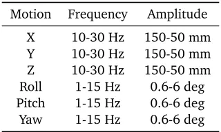
4.2 Road test parameters. . . 24

4.3 Rigid motion velocity scale factors for event CPG010. . . 30

4.4 Artificial motions. . . 36

4.5 Body CM and virtual accelerometer locations. . . 36

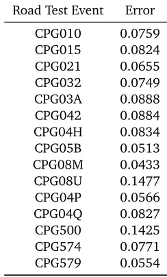
4.6 Drive file corresponding accelerations error for 15 events. . . 40

4.7 Drive file generation inputs. . . 44

4.8 Drive file generation outputs. . . 46

5.1 MATLAB®dynamic shaking inputs. . . 51

5.2 MATLAB®dynamic shaking outputs. . . 51

5.3 Powertrain-side accelerometer locations. . . 52

5.4 Powertrain inertia. . . 53

6.1 Linear bushing parameters. . . 56

6.2 Bushing rotational stiffnesses, MotionView®_{advanced model. . . . 56}

6.3 Bushing damping coefficients, MotionView®_{advanced model. . . . 56}

6.4 MotionView®_{DSTIFF Solver parameters. . . . 56}

6.5 Fatigue numbers of the six road test events, MotionView®_{and test. . . . 69}

6.6 Fatigue numbers of the front bushing vertical forces with ABM. . . 72

List of Figures

1.1 Multi-Axis Shaker Table. . . 2

1.2 Virtual Multi-Axis Shaker Table. . . 3

2.1 Vehicle simulated by Minaker and Rieveley[2]using their proposed method. . . 5

2.2 Virtual prototyping process by SBEL_[5_]. . . 6

2.3 Full vehicle test rig and basic test rig mechanics[23]. . . 15

3.1 Yaw, pitch and roll angles. . . 18

4.1 Schematic of chassis-side mount and accelerometer locations. . . 23

4.2 Drive file generation procedure. . . 25

4.3 Comparison between rigid and measured accelerations. . . 28

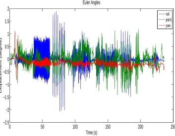
4.4 Euler angles of vehicle chassis derived for event CPG010. . . 31

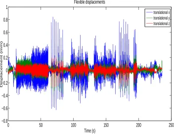
4.5 Flexible displacements on accelerometerAlocation. . . 32

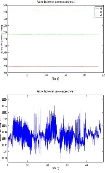
4.6 Relative displacements between accelerometers (above) and partial magnification (below). 33 4.7 Comparison between flexibility-considered and measured accelerations. . . 35

4.8 Comparison between simulated and artificial accelerations. . . 38

4.9 Comparison between flexibility-considered and measured displacements. . . 39

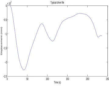
4.10 Typical drive file. . . 43

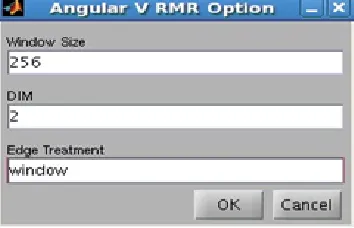
4.11 Angular velocity running mean removal dialog box. . . 44

4.12 RMS recovery dialog box. . . 45

5.1 Schematic of the VMAST and powertrain dynamic shaking model. . . 47

5.2 Side views and isometric view of the MotionView®model. . . 52

6.1 Roll angles of the powertrain, MATLAB®_{and MotionView}®_{. . . . 58}

6.2 Pitch angles of the powertrain and chassis from MATLAB®_{. . . . 59}

6.3 Powertrain CM translationalxacceleration, MATLAB®_{and MotionView}®_{. . . . 60}

6.5 Translationalx, yandzaccelerations on accelerometerA, MATLAB®_{and MotionView}®_{. . 61}

6.6 zaxis deflection of left front bushing, MATLAB®_{and MotionView}®_{. . . . 62}

6.7 zaxis deflection of right front bushing, MATLAB®and MotionView®. . . 63

6.8 zaxis load of left front bushing, MATLAB®and MotionView®. . . 64

6.9 zaxis load of right front bushing, MATLAB®and MotionView®. . . 64

6.10 Powertrain-side accelerations, MotionView®and test. . . 66

6.11 Left front bushingzaxial force, MotionView®and test. . . 67

6.12 Right front bushingzaxial force, MotionView®_{and test. . . . 67}

6.13 Rear bushingxaxial force, MotionView®_{and test. . . . 68}

6.14 Bushing forces fatigue data comparison for six events. . . 69

6.15 Left frontzaxial bushing force, ABM and test. . . 71

B.1 Bushing forces fatigue data comparison for nine events. . . 82

List of Abbreviations

All abbreviations used in this work are described in this section.

Abbreviation Meaning

ABM Advanced Bushing Model

ARDC Automotive Research and Development Center

BDF Backward Differentiation Formula

CM Center of Mass

DAE Differential Algebraic Equation

DOE Design of Experiments

DOF A Degree of Freedom

EOM Equation of Motion

FE Finite Element

FEA Finite Element Analysis

FWD Front Wheel Drive

GA Genetic Algorithm

GUI Graphical User Interface

LHS Left Hand Side

MAST Multi-Axis Shaker Table

MBD Multi-Body Dynamics

MBS Multi-Body System

NVH Noise Vibration Harshness

ODE Ordinary Differential Equation

RHS Right Hand Side

RMS Root Mean Square

VMAST Virtual Multi-Axis Shaker Table

Nomenclature

Mathematical nomenclature throughout this work is listed below, separated by the chapter in which it

first appears.

Literature Review

Label Description

f Vector of applied forces in global reference frame

h step size

K Kinetic energy

m Running mean removal window size

n number of points defined for running mean removal

~

n Applied torque vector in global frame

p₀ First data point in running mean removal

q Generalized coordinates

Q Generalized forces

t time

u Translational velocity

vp Velocity of the point of application of the external force F

x x coordinate

y ycoordinate

∆ Correction factor

Φ Constraint equations

λ Lagrange multiplier

~

ω Angular velocity vector

Theory

Label Description

~

aA Acceleration vector at locationA

~

aB Acceleration vector at locationB

~

aB/A Relative acceleration vector fromAtoB

~

aG Translational acceleration vector at the center of mass

a_xA,aA_y,a_zA Translationalx, y,zacceleration at locationA

~

F Total force vector acting on the center of mass

~

HG Angular momentum vector

I_{x x} Moment of inertia aroundx

I_{y y} Moment of inertia around y

I_zz Moment of inertia aroundz

Ix y Product of inertia aroundxandy

Ixz Product of inertia aroundxandz

Iyz Product of inertia aroundyandz

IG Inertia tensor

m Mass of the rigid body, a three by three diagonal matrix

~

MG Total torque vector acting about the center of mass

~r Coordinate vector of the global frame

~r_B/A Distance vector fromAtoB

~r₃ Coordinate vector of the rotating frame aroundx, yandz r_x Distance alongx

ry Distance along y

rz Distance alongz

R Transformation matrix from global to rotating frame

R₁ Transformation matrix from global to rotating frame (xonly) R₂ Transformation matrix from global to rotating frame (xandy) R₃ Transformation matrix from global to rotating frame (x, yandz)

~vA Velocity vector at locationA

~v_B Velocity vector at locationB

~v_B/A Relative velocity vector fromAtoB

~v_G Translational velocity vector at the center of mass

vx Translationalxvelocity in the rotating frame

vy Translational yvelocity in the rotating frame

x,y,z Coordinates of the global frame

x₁,y₁,z₁ Coordinates of the rotating frame aroundx only

x₂,y₂,z₂ Coordinates of the rotating frame aroundx andy x₃,y₃,z₃ Coordinates of the rotating frame aroundx,yandz

~α Angular acceleration vector in the body reference frame

αA x,α

A y,α

A

z Rotationalx,y,zacceleration at locationA

φ Euler angle aroundxaxis

θ Euler angle aroundy axis

~

ω Angular velocity vector of the body reference frame

ωx Euler angle rates aroundxaxis

ωy Euler angle rates around yaxis

ωz Euler angle rates aroundzaxis

ψ Euler angle aroundzaxis

Drive File Development

Label Description

~aA Acceleration vector at accelerometerA

~aB Acceleration vector at accelerometerB

~a_C Acceleration vector at accelerometerC I 3×3 identity matrix

˜

rA/G Skew-symmetric matrix representing distance from CM toA

˜

rB/G Skew-symmetric matrix representing distance from CM toB

˜

rC/G Skew-symmetric matrix representing distance from CM toC

v_{C M}s Filtered and scaled velocities at center of mass

vC M Filtered velocities at center of mass

aC M Accelerations at center of mass

vr x Rotational velocity aroundx

vr y Rotational velocity around y

v_rz Rotational velocity aroundz

a_m Measured accelerations

a_r Reproduced accelerations

Dynamic Shaking Model

Label Description

~a Powertrain translational acceleration vector at CM

C Bushing damping coefficient

E Euler angles

~

F Total force vector at powertrain CM

~

F_B Bushing force vector

g Gravitational constant

K Bushing stiffness

~

MG Total moment vector at powertrain CM

~

MH Half-shaft torque vector

~r Distance vector from powertrain CM to powertrain-side mount loca-tions

~v Powertrain translational velocity vector at CM

~v_e Powertrain-side mount location velocity vector in the local frame

~v_f Chassis-side mount location velocity vector in the global frame

~

x Powertrain CM location vector in the global frame

~

xe Powertrain-side mount location vector in the global frame

~xf Chassis-side mount location vector in the global frame

~α Powertrain angular acceleration vector at CM

~

Chapter 1

Introduction

1.1

Motivation

The multi-axis shaker table (MAST) (Figure 1.1), has been widely used in the automotive industry in

order to test vehicles or vehicle components specifically under high frequency excitation for various

purposes, such as fatigue analysis, ride quality and noise vibration harshness (NVH). As one of the major

tasks of the MAST, the fatigue test is vital for vehicle design engineers in carrying out quality products

while maintaining minimum cost. One common example is the powertrain (engine and transmission

assembly) mount durability test, in which the powertrain is mounted on the vehicle frame through

bushings; the whole assembly is then fastened to the shaker table platform, which is driven by hydraulic

cylinders. Acceleration data collected on the vehicle frame during the road test is used as the target

output for the shaker to match, and the feedback loop control algorithm is implemented to automatically

adjust the actuation force. However, conducting such a test requires both hardware and time: prototype

vehicles have to be built, the test rig must be set up, and the test cycle lasts for hours and hours.

To this end, the Chrysler Automotive Research and Development Center (ARDC) and University of

Windsor have worked together in a research project to develop a virtual simulation tool that could

numerically simulate the shaking process of a vehicle powertrain and predict the powertrain mount

loads. The ultimate goal of this project is to replace the physical shaking test with virtual shaking

simulation that could precisely predict the vehicle chassis and powertrain motion, as well as mount

loads. By virtually changing the powertrain and mount parameters, new simulation results would be

Figure 1.1:Multi-Axis Shaker Table.

1.2

Virtual Multi-Axis Shaker Table

The virtual multi-axis shaker table (VMAST) is a simulation tool developed to numerically simulate the

vehicle powertrain behavior under real road input profiles in order to acquire powertrain mount load

data. The simulation result can be used to predict the fatigue of the bushing mount. It is a user friendly

software package, and it has the advantage of changing the physical properties with ease, which allows

rapid design iterations.

Designed to function the same as the physical shaker table, the VMAST is able to cover full six

de-grees of freedom (DOF) rigid motions of the shaker platform (three translational and three rotational).

In addition, it has the capability to recover local deformation on the vehicle frame by introducing extra

translational degrees of freedom. The VMAST reads in acceleration data of the vehicle frame collected

from the proving ground, and transfers it to displacement for the purpose of driving the dynamic

shak-ing. Mathematically, the total number of degrees of freedom that the virtual shaker can produce is

identical to the number of input accelerations. For example, a vehicle frame that has three

accelerom-eters on distinct locations will give nine translational accelerations. The shaker can then solve for nine

displacements. The combined motion of the nine displacements contains the chassis rigid motion and

the local deformation. A schematic of the VMAST is shown in Figure 1.2; the red arrows represent the

rigid motion that the shaker could produce, and the yellow arrows demonstrate the overall degrees of

freedom the shaker generates, which consist of rigid and flexible.

The VMAST reproduced time history coordinate data is called the ‘drive file’, as it is used to drive the

dynamic shaking. The generation of the drive file will be explained in detail later in the thesis, and is

Figure 1.2:Virtual Multi-Axis Shaker Table.

1.3

Virtual Dynamic Shaking

After the drive files are developed, the next step is to conduct the dynamic shaking and collect the

result. There are two components to make up the dynamic shaking model: the powertrain and bushing

mounts. This model treats the powertrain as a single rigid body with moments and products of inertia,

that is connected to the bushing mounts. The model can be built and simulated using MATLAB®_{. In}

case a more complex powertrain model is needed, commercial software such as MSC® Adams® or Altair®MotionView®can be used to construct the advanced model where, for example, the powertrain model may be equipped with additional linkages. Both simple and complex models are able to generate

simulation results such as the powertrain local acceleration, velocity and displacement, as well as the

bushing travel for powertrain motion study, and the bushing force for fatigue analysis.

Depending on the requirements of the simulation, either a simple or sophisticated bushing model can

be used. The simplest bushing model uses linear stiffness and damping based on a reasonable estimation,

which is computationally fast. The advanced bushing model (ABM) can be applied in the simulation

where the most accuracy is needed. It is a virtual bushing model with a parameter identification tool,

which identifies the virtual bushing parameters based on real bushing test data. However, it is relatively

time consuming.

1.4

Research Objectives

The first objective is to develop a set of MATLAB®_{codes that generate the desired motion to drive the}

powertrain. The codes must be able to read the acceleration data collected on the vehicle frame during

the road test and reproduce the motion of the vehicle frame. The process should virtually replay the

vehicle frame motion due to excitation from the road in the real case.

of the powertrain. The model reads in the motion produced in the first step, simulates and generates the

time history output. This numerical model is compiled to be a user friendly design tool in cases where

the powertrain mechanism is simple. It is easy to implement and is capable of running in batch mode.

The last objective is to use MBD software for complex powertrain mechanism modeling and

simula-tion. In this case, the shaker and powertrain models need to be built with commercial software.

1.5

Structure of the Thesis

The thesis consists of seven chapters. The first chapter introduces and describes the motivations and

goals of the research, as well as the research product and its function. The second chapter is a review

of the literature, which includes a review of the virtual simulation tools and their corresponding solving

algorithms, as well as the previous research in the relevant area. In Chapter 3, the theory used to develop

the virtual shaker will be addressed.

In Chapter 4, the drive file development approach is introduced, which includes five detailed steps

of the numerical approach to reproduce the vehicle frame motion from accelerations in order to drive

the dynamic shaking. The chapter will focus on the application of relevant mathematical algorithms,

as well as the data processing method, e.g., the data filtering. In addition, a validation is included,

and the assumptions and limitations are also discussed. Lastly, the software application of the drive file

development process is described.

In the first half of Chapter 5, the MATLAB®dynamic shaking model is presented. The kinematic and dynamic equations used to solve the model are introduced. The limitation of the MATLAB®model is also discussed. In addition, the software application of the MATLAB® model is described. The second half of this chapter is focused on the model built using MBD commercial software. An Altair®MotionView® shaker and powertrain model is presented. The physical parameters of the vehicle and powertrain model

are from the Chrysler PF platform with a 2.4L engine.

In Chapter 6, the simulation and results of both MATLAB® _{and MotionView}®_{models are discussed.}

The validation of the simulation results is done through the following: a check on the plausibility of the

simulation results in the real world; comparison of the simulation results between the virtual models;

comparison of the simulation results against test data.

In Chapter 7, conclusions on the development and application of the VMAST are presented. Potential

Chapter 2

Literature Review

2.1

Multi-Body Dynamics

The use of multi-body dynamics (MBD) is essential in vehicle design and testing. According to Schwerin[1],

multi-body systems (MBS) play an important role in computer aided technical mechanics, and vehicle

dynamics is the major area of application. The ability to design and optimize such technical multi-body

systems gives a company working in this area the competitive edge on the market. The equations of

motion (EOM) are well known to describe the behavior of a multi-body system as a set of mathematical

functions in terms of dynamic variables. Much work has been done on studying multi-body systems for

automatic generation of the equations of motion, for example, see Minaker and Rieveley_[2_]. A method

was developed for automatic generation of linearised equations of motion that allows for easy

inclu-sion of nonholonomic constraints, and the method presents equations of motion well suited for vehicle

stability analysis. They stated that the use of mathematical models in vehicle system design has grown

immensely in recent history, leading to the development of models with increasing size and complexity.

2.2

Virtual Simulation

As Grote and Sharp[3]stated, the past decades have seen a rapid advance in computer based prediction

and analysis tools. These tools allow for parts and assemblies to be constructed and their behavior

predicted in the virtual world of computer simulation. Becker, Salvatore and Zirpoli[4]pointed out that

virtual simulation tools now play a very important role in new product development. They have been

widely hailed to significantly cut development time and costs. They argued that the contribution of

virtual tools to experimentation goes well beyond the incremental improvement of the results obtained

with physical experimentation. “Virtual simulation techniques can do much more than just reduce the

cost and increase the speed of problem solving,” they mentioned.

2.2.1

Modeling Techniques

ADAMS

The Automated Dynamic Analysis of Mechanical Systems (ADAMS) software marketed by MSC® Soft-ware has been proven as very beneficial to virtual prototype development (VPD) by reducing product

time to market and product development costs.

As proposed by the Simulation Based Engineering Lab (SBEL)[5], the virtual prototyping process of

ADAMS®_{includes four steps. The first step is building a model using bodies, joints, contacts and forces.}

The next step is testing the design using measures, simulations, animations and plots; the simulation

result can be validated by importing test data and superimposing it. Next, one should review the design

by adding friction, forcing functions, flexible parts and control systems, and iterate it through parameters

and design variables. Lastly, the design is improved using DOEs (Design of Experiments) or optimization.

The design process can be automated by using custom menus, macros or custom dialog boxes. This

modeling strategy is not only valid in ADAMS®, but also in other multi-body codes as well.

Figure 2.2:Virtual prototyping process by SBEL[5].

MotionView

has the advantage of a particularly user friendly GUI (Graphical User Interface), and better graphical

representation when comparing with ADAMS®_{. Its capability in handling nonlinear elements, such as}

flexible beams or bushings, as well as modeling complex multi-body system, like a vehicle chassis

as-sembly is competitive with ADAMS®. It has been gaining popularity among engineering companies and academic institutions, especially for those who want to model and simulate multi-body systems

with-out much proficiency or experience. The modeling technique described above is well suited for the

MotionView®application.

The MotionView® _{default solver—MotionSolve}®_{, is a system level, multi-body solver that is based}

on the principles of mechanics_[7_]. Using a multi-body system built in MotionView®_{, MotionSolve}®

automatically formulates the equations of motion and numerically solves them. MotionSolve®_provides

four types of simulation: transient, static, quasi-static and linear, among which transient is used to

dynamically simulate the system with more than zero degrees of freedom. The names of the solvers

used for solving differential algebraic equations (DAEs) in transient simulation are: ABAM, VSTIFF,

MSTIFF and DSTIFF. The default solver is DSTIFF. It is claimed in the research that the DSTIFF solver

is more robust than the solvers in ADAMS® in dealing with high frequency excitation as an input to multi-body systems.

MATLAB

According to Hanselman and Littlefield[8], MATLAB®was initially developed by a lecturer in the 1970’s to help students learn linear algebra. Later, it was marketed and further developed under MathWorks® Inc. MATLAB® is a software package that can be used to perform analysis and solve mathematical and engineering problems. It has excellent programming features and graphics capability that are easy to

learn and provide the user with great flexibility. SIMULINK®—a data flow graphical programming tool, is used for modeling, simulating and analyzing dynamic systems. It has a comprehensive library that can

be used to simulate linear, non-linear or discrete systems. The programming features and comprehensive

mathematical functions enable the modeling of complex MBS in the MATLAB®_environment.

Other commercial software such as MapleSim® _{and CarSim}® _{might be applicable for the research}

presented in this thesis. However, due to the adequate number of approaches already available, the

software is not further studied.

2.2.2

Solving Algorithm

After the MBS is built in the pre-processor, the next step is to simulate the system. Once the simulation is

initiated, the MBD software will analyze the information that the user imports, such as the generalized

coordinates, constraints, motions and initial conditions. Depending on the simulation type chosen, the

next step is to formulate the corresponding equations of motion of the system. In terms of dynamic

Negrut and Dyer[9]. According to them, the Lagrange formulation of the equations of motion is shown

as the following second order differential equations

d d t

–_∂K

∂˙q T™

− ∂_K

∂q T

+ ΦT

qλ=Q (2.1)

where:

K=kinetic energy

q=generalized coordinates

Φ =constraint equations

λ=Lagrange multiplier

Q=generalized forces

The second order equations can be further reduced to first order considering the choice of the

gen-eralized coordinates q=    p "    (2.2)

wherepis the positon and"is the orientation (Euler angles). The first order equations are shown as:

d d t



 

€_∂K

∂u ŠT _∂ K ∂ ζ T   −    ∂K ∂p T

€_∂K

∂ " ŠT   +    ΦT pλ ΦT "λ   =    (Q p)T_f (Q

R)T_¯n 



 (2.3)

The projection operators in the generalized forces term are computed as:

Y p=∂v

p

∂u (2.4)

Y

R= ∂ ~ω

∂ ζ (2.5)

where:

u=translational velocity

ζ=Euler angle rates

f =vector of applied forces in global reference frame

n=applied torque in global frame

vp=velocity of the point of applicationPof the external forceF

~

Since d d t ∂_K ∂u T

=Mu˙ (2.6)

∂_K

∂p T

=0 (2.7)

with the angular momentum defined as:

Γ =∂_{∂ ζ}K =BT~J Bζ˙ (2.8)

the EOM of Eq. (2.3) are reformulated as:

Mu˙+ ΦT_pλ=Yp T

f (2.9)

Γ−∂K

∂ " + Φ

T

"λ=

Y R

T

¯

n (2.10)

The first order differential equations above are called in what follows kinetic differential equations,

and they indicate how external forces determine the time variation of the translational and angular

momentum.

At last, the time variation of the generalized coordinates is related to the translational and angular

momentum by means of thekinematic differential equations. By assembling the kinetic and kinematic

differential equations, a set of equations for each rigid body in the MBS are derived as follows:

Mu˙+ ΦT_pλ₋Yp T

f =0 (2.11)

Γ−BT~J Bζ=0 (2.12)

Γ−∂K

∂ " + Φ

T

"λ−

Y R

T

¯

n=0 (2.13)

˙

p₋u=0 (2.14)

˙

"−ζ=0 (2.15)

It is notable that the solution to the above differential equations must also satisfy the kinematic constraint

equations of the system. The equations are:

Φ q,t

=0 (2.16)

Φq q,t ˙

q=−Φt q,t

(2.17)

Φq q,t ¨

q=−€Φq˙qŠ

q˙q−2Φqtq˙−Φt t q,t

This set of differential and constraint equations from Eq. (2.11) to Eq. (2.18) are called the

Differ-ential Algebraic Equations (DAEs). In many cases, the DAEs of the MBS cannot be solved symbolically.

Therefore, a numerical solution is used find a close approximation. As Negrut and Dyer stated[9], the

most common DAE solver that ADAMS®uses is the GSTIFF-I3. Here the GSTIFF stands for the solution of stiff differential equations, and I3 means the index of the DAEs is three, which means the number

of times the constraints in the system must be differentiated to get the system into ODEs is three. It is

always index three for a mechanical system. In mathematics, a stiff equation is a differential equation

for which certain numerical methods for solving the equation are numerically unstable, unless the step

size is taken to be extremely small. Lambert_[10_]described stiffness as: “If a numerical method with a

finite region of absolute stability, applied to a system with any initial conditions, is forced to use in a

cer-tain interval of integration a step length which is excessively small in relation to the smoothness of the

exact solution in that interval, then the system is said to be stiff in that interval.” According to Gear and

Skeel[11], the earliest paper on stiff differential equations was given by Curtiss and Hirschfelder[12],

in which they developed the method using backward differentiation formula (BDF) in solving

differ-ential equations that failed to come up with stable numerical solutions with other methods. The next

significant development was the definition of A-stability by Dahlquist[13]. The theory was extended

by Daniel and Moore[14], mentioning that the order of an A-stable method cannot exceed twice its

number of derivatives involved implicitly in each step. Later approaches including Widlund_[15_]and

Gear[16][17] focused on breaking through the order limitation implied by A-stability. Both of them

explored non-A-stable methods, which were realized to be most effective for general stiff problems.

When solving the DAEs, GSTIFF-I3 will first apply an order one implicit integration formula, in order

to convert the DAEs into a set of algebraic equations. The one step, A-stable BDF replaces the derivative

˙

y₁at timet₁with

˙y₁=1 hy1−

1

hy0 (2.19)

Then the derivative in the above equation can be ‘discretized’ by replacing ˙y₁with a nonlinear function

g(y,t). The equation becomes:

1

hy1−

1

hy0−g(t1,y1) =0 (2.20)

To retrieve y₁, this ‘discretization equation’ is solved using a Newton-Raphson type iterative algorithm as follows:

x(1)=x(0)₋ f(x

(0)₎

f0_(x(0)₎ (2.21)

The algorithm continues by settingx(0)withx(1).

By applying the discretization approach to Eq. 2.11 to 2.15 and the position constraint equation form

At this stage, the unknowns in the nonlinear equations are defined as:

yT=h u Γ ζ p " λ f n¯ iT

(2.22)

the nonlinear system is rewritten as:

Ψ(y) =0 (2.23)

The Newton-Raphson method is then used to solve the system. Once the initial value of y(0)is predicted, the iteration runs as:

Ψy(y0)∆(j)=−Ψ(y(j)) (2.24)

y(j+1)= y(j)+ ∆(j) (2.25)

until the correction∆(j)_{are small enough (the value of∆is set by the user).}

Competitive with the ADAMS® solver, MotionSolve® dynamic simulation accounts for all inertia effects, all applied forces and internal constraints. In dynamic simulations, the MotionSolve® solver analyzes the MBS and generates a set of DAEs. It solves the equations of motion in their most general

form, including nonlinear effects[7]. The default DAE solver that MotionSolve®uses is DSTIFF, and the default setting for the DAE index is 3, which means the position constraint is included. According to

the MotionSolve®_{reference guide[18], it solves a system of differential/algebraic equations of the form}

G(t,y,y0) =0, using a combination of BDF methods. This method is based on the available integrator DASPK, which is developed by Brown, Hindmarsh and Petzold[19].

2.2.3

Data Processing

Virtual simulation uses the data collected externally to reproduce the real case. However, as mentioned

by Pyle[20], the data-gathering methods are often loosely controlled, resulting in out-of-range values,

impossible data combinations, missing values, etc. Analyzing data that has not been carefully screened

for such problems can produce misleading results. Thus, the representation and quality of data is

im-portant.

The acceleration data that VMAST reads in is a high frequency, time-history signal collected from

tests in the proving grounds. The data sometimes has undesired high frequency content that could

lead to a nonsensical outcome if further processed. Another source of data error faced in the shaker

developing process is the integration constant, which is an ambiguity inherent in the construction of

antiderivatives. It is an arbitrary constant that affects the accuracy of the integration result.

In order to obtain accurate and meaningful simulation results, the input data and intermediate results

must be properly processed. Two methods are studied and found effective in eliminating the numerical

Butterworth Filter

The Butterworth filter is a type of signal processing filter designed to have as flat a response as possible

in the passband. It is also referred to as a maximum flat magnitude filter. The filter was first described

by Butterworth[21] stating: “An ideal electrical filter should not only completely reject the unwanted

frequencies but should also have uniform sensitivity for the wanted frequencies.”

The frequency response of the Butterworth filter is maximally flat in the passband and rolls off

towards zero in the stopband. The advantage of the Butterworth filter is that it is very good at simulating

the passband of an ideal filter. In other words, it gives the minimum distortion in the passband. However,

as it goes to zero gradually, some parts of the stopband are still kept. As the design characteristic of the

Butterworth filter, the filter order, which is defined as the maximum delay (in samples) used in creating

each output sample, can be increased to enable a better filtering performance.

As a result, the low pass Butterworth filter is a good choice for eliminating the high frequency content

buried in the acceleration data while preserving the desired frequencies in order to gain maximum

accuracy in the simulation.

Running Mean Removal

The running mean is a calculation to analyze data points by creating a series of averages of different

subsets of the full data set. Commercial software, such as nCode GlyphWorks®[22] and MATLAB® provide the function of auto generation of the running mean on each data point. It works based on

the user selected number of pointsn. Starting from the first data point p₀, this function calculates the average of a ‘window size’m, wherem=2n+1, and the length of the window being calculated ranges

fromp₀−ntop₀+n. Then the calculation proceeds to the next data point until it reaches the last one. When calculating the first or the last group ofndata points, the size of the window exceeds the size of

the data points available. Thus, there are several options of padding the edge of the data. They are:

‘edge’, which pads the data with the first and last values; ‘zero’, which pads the data with zeros; ‘mean’,

which pads the data with the mean of the subset; ‘window’, which pads the data with the first half and

last half window.

Once the mean is obtained, the next step is to subtract it from each data point. This function is to

remove the trend from the signal, which appears as the integration constant on the intermediate result

during the ‘drive file’ generation procedure.

2.3

Previous Work

As Dressler, Speckert and Bitsch mentioned_[23_], in recent years so-called ‘virtual test rigs’ have become

more and more important in the development of cars and trucks. Originally, the idea was to substitute

cooperative usage of numerical and laboratory rig simulation. In the early development stages, when no

physical prototypes are available yet, numerical simulation is used to analyze and optimize the design.

2.3.1

Quarter-Car Test Rig

Many papers have been published on the development of virtual test rigs for vehicle component tests.

One of them was by Sandu, Andersen and Southward[24], in which they developed a multi-body

dy-namics model of a quarter-car test rig equipped with a McPherson strut suspension. Both linear and

nonlinear models were developed in order to predict the dynamic response of a quarter car suspension.

The linear model consists of a sprung mass, an unsprung mass, and wheelpan actuator plate bodies.

The sprung mass is supported by the primary-ride spring and included mass from the sprung mass plate

and strut tower. The assumptions made for the linear model is that the motion of the masses could be

approximated as linear translational. Also, the springs used in the system are assumed to have linear

behavior. The equations of motion of the model are formulated by using the Lagrange multiplier to

assemble the constraint forces with the inertia forces.

The major difference between the linear and nonlinear models is that the nonlinear model accounts

for the kinematic joint constraints. Instead of positioning the sprung and unsprung mass in the uniform

vertical direction, the unsprung mass is connected to the sprung mass through control arms, which

breaks the geometrical linearity. The structure is assumed to be rigid. The same algorithm was used to

formulate the nonlinear system equations.

The HHT method integrator was used to solve the DAEs of both the linear and nonlinear models,

and the simulation results were compared against experimental data. The performance metric chosen

to judge how well the mathematical model predicts reality is the ratio of the root-mean-square (RMS)

of the error between simulation and experimental results to the experimental RMS. It is shown in the

paper that both linear and nonlinear models predict the dynamic response of the quarter car model,

such as the accelerations of both the sprung and unsprung masses, and the nonlinear model has better

performance. The simulation result can be further implemented in studying the dynamic behavior of

other nonlinear components, like dampers and bushings.

2.3.2

Full Vehicle Test Rig

The virtual test rig brought by Mántaras and Luque[25]focused on investigating the three-dimensional

position of the vehicle body (i.e., roll, pitch and height of the center of gravity) and the main parameters

(e.g., caster, camber, steer angle, kingpin inclination, toe in/out, roll axis, bump steer, Ackerman angle),

that influence the handling of the vehicle. They proposed a three-dimensional kinematic model of the

front and rear suspension and the steering system, in order to predict the vehicle positions as well as the

First of all, the coordinate frames are determined. One reference frame is attached to each wheel,

plus a reference frame for the vehicle and a global reference frame (non-moving or inertial). The

orientation of the vehicle is defined using Cardan angles. The next step is to determine the kinematic

equations of each component. The kinematic equations of each wheel are determined using the

three-dimensional constraint equations for the point of origin of the reference frame. The movement of the

rear axle, in spite of being a three-dimensional movement, is considered as a combination of two plain

movements. The vehicle kinematic model is built based on the assumption that the road is a plane, so

the calculation of a plane tangent to the wheels can be used. At this stage, the full vehicle model is

developed and ready for a virtual test.

The virtual test rig was set up using MATLAB® _{and Simulink}®_{. The geometric parameters of the}

vehicle components are pre-defined by the user. The inputs to the test rig are, as a function of time, the

roll angle and pitch angle of the vehicle body, the vehicle center of gravity height and the steering angle.

The outputs of the simulation are the vehicle camber, caster, etc., which can be fed back to the system to

optimize the vehicle geometry.

The author validated the virtual test rig simulation result against a measured result, where a small

difference can be anticipated in the comparison, this being essentially a function of errors of

measure-ment associated with the instrumeasure-ments used. Also, a MBS vehicle model was built in ADAMS®to validate the virtual test rig.

Another full vehicle virtual test rig was introduced by Dressler, Speckert and Bitsch[23]. In their

paper, the numerical simulation models of complex servo-hydraulic test systems and their test specimen

were demonstrated. The full vehicle test rig is composed of four hexapod-based suspension test rigs.

The hexapod technology was illustrated by driving a platform that is connected to the wheel hub using

six actuators; thus, the platform supports all six DOF of the hub. At a closer look, the hexapod consists

of a base and a top platform, which are connected via six identical actuators. The joints between the

actuators and the platforms have two rotational DOF. One actuator contains the piston and the cylinder,

which in turn are connected using a cylindrical joint. This construction contains six DOFs. The force

and torque balance equations of the construction are listed and imported into MATLAB®to calculate the actuator forces for certain suspension tests. The full vehicle model has one hexapod test rig connected to

each wheel hub. Besides, each individual test rig is upgraded to have an additional six DOF, representing

the tire model.

The research team also carried out physical test track simulations to compare with virtual

simula-tion in results on forces, accelerasimula-tions and displacements, as well as damage-related histograms, e.g.,

rainflow counting, range pair counting and damage values.

As a conclusion, current virtual test rigs are capable of producing quality simulation results that

can be used in accelerating the design process and to contribute to a more cost and time efficient test

Figure 2.3:Full vehicle test rig and basic test rig mechanics[23].

behavior, and virtual simulation studies of the vehicle powertrain’s (engine and transmission assembly)

dynamic behavior under external excitation have been sparse. The research presented in this paper

aimed to build a virtual test rig to simulate the vehicle powertain dynamic response under road input

Chapter 3

Theory

A series of kinematic and dynamic theories used in the drive file generation procedures and virtual

shaker model development are introduced in this chapter, including the rigid body kinematics,

coordi-nate transformation and equations of motion.

3.1

Rigid Body Kinematics

In physics, a rigid body is an idealization of a solid body in which deformation is neglected. In other

words, the distance between any two given points of a rigid body remains constant in time regardless

of external forces exerted on it. In this way, the kinematic relationships between any two points are

studied.

There are two important relationships. First, the relationship of translational velocity between two

points is formulated as:

~vB=~vA+~vB/A (3.1)

where_~vB/Ais the is the relative velocity, and it can be represented as:

~v_B/A=ω~_×~r_B/A+~˙r_B/A (3.2)

where:

~

ω=angular velocity of the body reference frame

~rB/A=distance vector fromAtoB

It is worth pointing out that the angular velocity is the same for any point fixed to the body. If pointA

and pointBare both fixed to the same body, then~˙rB/A=0.

The equation of acceleration between two points is:

~

aB=~aA+~aB/A (3.3)

where~aB/Ais the is the relative acceleration, and it can be represented as:

~

a_B/A=~α_×~r_B/A+ω~_׀ω~_×~r_B/AŠ+2ω~×~˙r_B/A+~¨r_B/A (3.4)

where:

~α=angular acceleration of the body reference frame

~

ω=angular velocity of the body reference frame

~r_B/A=distance vector fromAtoB

~˙rB/A=rate of change of~rB/Ain the rotating frame

~¨rB/A=rate of change of~˙rB/Ain the rotating frame

The four terms in the RHS following the sequence are called the tangential acceleration, the centripetal

acceleration, the Coriolis acceleration and the radial acceleration. For a rigid body whose angular

veloc-ity is very small, the centripetal acceleration term can be neglected as the square product of the angular

velocity approximately equals to zero. The Coriolis acceleration is generated by the Coriolis effect, which

is a deflection of moving objects when they are viewed in a rotating reference frame. So if observed from

the rigid body local frame, the point on the rigid body has no Coriolis effect and the Coriolis acceleration

term can be neglected. Also, the last term is zero for a rigid body. Thus, Eq. (3.3) can be rewritten as:

~

a_B=~a_A+~α_×~r_B/A (3.5)

In the three dimensional coordinate system, the acceleration of point A forms the vector as:

~a_AT= [ aA_x aA_y aA_z ]T (3.6)

Also, the angular acceleration is written as:

~αT

A = [ αAx α A y α

A z ]

T

(3.7)

Similarly, the acceleration at pointB can also be written as a vector form. If the LHS of Eq. (3.5) is

third point on the rigid body is known, then there are six known value against six unknowns. The number

of knowns is equal to the number of unknowns, and the system seems determined. However, there is

redundancy in the equations. Thus, the accelerations of at least one additional point are required to solve

the system, but there will be nine knowns against six unknowns, and the system is overdetermined. The

least squares method is then used to approximate the solutions.

3.2

Coordinate Transformation

The rotation of a rigid body is often described using an angular parameter such as angular displacement,

velocity and acceleration, with respect to the body reference frame. Yet, the pure translational motion

is described with respect to a coordinate frame that is fixed. So when there is both translational and

rotational motion, a method is applied to transfer the coordinates from a rotating frame into a fixed

frame. In order to describe the method, the concept of Euler angles is first introduced. The Euler angles

Roll

Yaw Pitch

Figure 3.1:Yaw, pitch and roll angles.

are three angles introduced by Leonhard Euler to describe the orientation of a rigid body. They are

typically denoted asψ, θ andφ. The three angles represent a sequence of three elemental rotations, i.e., rotations about the axes of a coordinate system. In the automotive industry, the yaw-pitch-roll angles

are often used to describe vehicle orientation (Figure 3.1). When calculating the orientation, the Euler

angles work in the selected sequence. In a three dimensional coordinate system, the yaw-pitch-roll (also

called 3-2-1) sequence transforms the coordinate in the following way: first, the frame rotates aroundx

axis with an angle_φ. The geometric relationship between the new coordinates and the old ones is:

     x₁ y₁ z₁      =      

1 0 0

0 cosφ sinφ 0 −sinφ cosφ

wherex₁, y₁andz₁are the new coordinates. The next step is to rotate around y axis with an angleθ. The coordinates derived in the last step are used as the datum in this rotation, and the formulation is:

     x₂ y₂ z₂      =      

cosθ 0 −sinθ

0 1 0

sinθ 0 cosθ            x₁ y₁ z₁      (3.9)

In the last step, the reference frame rotates aroundzaxis with an angleψ, whose equation is as follow-ing:      x₃ y₃ z₃      =      

cosψ sinψ 0

−sinψ cosψ 0

0 0 1

           x₂ y₂ z₂      (3.10)

The equations above can be written in the form:

~r₃=R₃R₂R₁~r (3.11)

where R₁,R₂ and R₃ are the transformation matrix in Eq. (3.8), (3.9) and (3.10) respectively. The product of the three matrices formulates the final transformation matrix. It describes the rotations

regarding a rotating frame. If the rotations are about space fixed axes, the order of the rotations is

reversed and the transformation matrix becomes the following; see Baruh[26].

R=R₁R₂R₃=      

cψcθ s_ψcθ −s_θ −sψcθ+cψsinθsφ cψcφ+sψsθsφ cθsφ

sψsφ+cψsθcφ −cψsφ+sψsθcφ cθcφ       (3.12)

wheres=sinandc=cos.

Similarly, the Euler angle rates (first derivative of Euler angles) have the following relationship with

the angular velocity:

ωx=φ˙−ψ˙sinθ (3.13)

ωy=θ˙cosφ+ψ˙cosθsinφ (3.14)

ωz=−θ˙sinφ+ψ˙cosθcosφ (3.15)

where:

~

ω=angular velocity expressed in the body fixed frame

     ˙ ψ ˙ θ ˙ φ      =      

0 sinφ/cosθ cosφ/cosθ 0 cos_φ −sin_φ 1 sinφtanθ cosφtanθ

           ωx ωy ωz      (3.16)

If the angular velocities of the rigid body are known, the above equations become ODEs and the Euler

angle rates and Euler angles can be solved using an ODE solver.

3.3

Equations of Motion

The equations of motion are equations that describe the behavior of a MBS in terms of its motion as a

function of time. The equations for translation

X

~

F=m~aG (3.17)

where the subscriptG stands for the center of mass, work equally well in two dimensional and three

dimensional coordinate systems. However, the rotational equations are not so simple. First, the moments

of inertia are defined as:

Ix x = Z

r2_y+r_z2d m (3.18)

Iy y= Z

€

r2_x+r_z2Šd m (3.19)

I_zz= Z

r2_x+r2_yd m (3.20)

whereri(i=x,y,z)is the length along the coordinate axes, andmis the mass of the object. Also, the

cross-products of inertia are defined as:

I_{x y}= Z

r_xr_yd m (3.21)

I_xz= Z

r_xr_zd m (3.22)

I_yz= Z

r_yr_zd m (3.23)

Now the inertia can be written into a matrix from as:

I=      

Ix x −Ix y −Ixz

−Iy x Iy y −Iyz

whereI is called the inertia tensor. The angular momentum is expressed as:

~

HG=IGω~ (3.25)

The combined translational and rotational dynamics of a rigid body can be expressed by the

Newton-Euler equations:

X

~

F=m~˙vG+ω~ ×m~vG (3.26)

X

~

M_G=I_G~α+ω~_×I_Gω~ (3.27)

where:

~

F=total force acting on the center of mass

m=mass of the rigid body, a three by three diagonal matrix

~vG=translational velocity of the center of mass

~˙vG=translational acceleration of the center of mass

~

MG=total torque acting about the center of mass

IG=inertia tensor

~α=angular acceleration

~

ω=angular velocity

The second term on the RHS of Eq. (3.26) is considered if a rotating frame is used for~v. The total torque is the derivative of the angular momentum, and the second term in the RHS is called the gyroscopic

moments.      ˙ x ˙ y ˙ z      =R      vx vy vz      (3.28)

Note thatP~FandPM~ are functions ofx,y,z,ψ,θ,φand their derivatives, thus an ODE solver is also required. In addition, the velocity in the body fixed frame has the relationship with the displacement

in the global frame shown in Eq. (3.28), whereRis the transformation matrix which transforms the

Chapter 4

Drive File Development

4.1

Displacement Driven Simulation

The VMAST resembles the real shaker by matching the test accelerations. However, instead of adjusting

the acceleration magnitude with a feedback loop, it uses time-history displacement signals which are

recovered from the test accelerations, and their corresponding accelerations closely match those from

the test, which promises the accuracy of the simulated inertia load.

It seems more time efficient to drive the dynamic simulation with accelerations directly, as the

dis-placement conversion is omitted. In fact, the experimental results showed that the test acceleration is

not suitable for driving the simulation. First of all, the test accelerations can not be used unprocessed,

as the numerical errors buried in the data are destined to cause faulty results. However, the numerical

processing on the acceleration data is not easily done because there is no criterion as a reference. Unlike

displacements, which represent some physical relationships, such as the chassis rigidity and orientations

that can be easily observed and controlled, the accelerations don’t obviously reveal such relationships.

Thus, it is very challenging to control the numerical processing on the acceleration data, and this is why

the accelerations have to be converted.

The number of driving displacement signals depends on the number of accelerometers that were

used to collect the test accelerations. The accelerometer records data in its own coordinate frame on the

three axial directions (x, yandz). If the vehicle chassis motion was recorded by three accelerometers,

the driving displacement should correspondingly have nine signals.

4.2

Drive File Development

This section describes the details of the conversion from acceleration to displacement. The powertrain

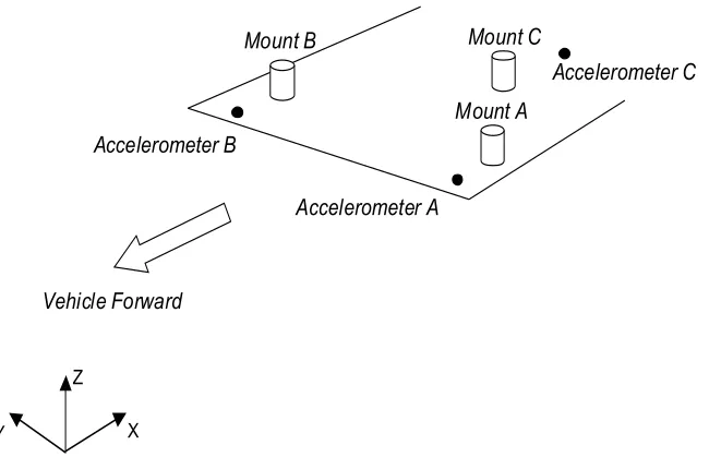
indoor road test data, collected on Chelsea Proving Grounds). This transverse powertrain has three

mounts (each labeled asA, B andC), two of which are in the front, supporting the engine. The left

and right side are defined by the driver’s view while sitting in the driver’s seat. The last one holds the

transmission. The accelerometers are installed on the vehicle chassis right beside the mount locations,

and labeled asA,B andC; see Figure 4.1. The road profile contains nine pieces of acceleration data.

Each three describe the axial translational accelerations of one accelerometer in its local coordinate

frame. The input parameters were measured in a global fixed frame, see Table 4.1 and 4.2 for details.

It is worth pointing out that although the initial location of the accelerometers were measured in a

different coordinate frame than accelerations, there is no conflict as the locations are only used to find

out the relative distance.

$

$

$

$

$

$

$

$ $ $

!!"#"$%&"'"$()_$

($

)$ *$

!!"#"$%&"'"$( _$ *%+,'()_$

*%+,'( _$ *%+,'(-_$

!!"#"$%&"'"$(-_$

."/0!#"(1%$23$4_$

Figure 4.1:Schematic of chassis-side mount and accelerometer locations.

Table 4.1:Vehicle chassis parameters.

Item Name Location_[x,y,z] [mm_] Item Name Location_[x,y,z] [mm_]

Left Front Mount A [-182,-453,370] Left Front Accelerometer A [-590, -455, 280] Right Front Mount B [-200, 492, 391] Right Front Accelerometer B [-590, 490, 280]

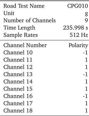
Table 4.2:Road test parameters.

Road Test Name CPG010

Unit g

Number of Channels 9 Time Length 235.998 s Sample Rates 512 Hz

Channel Number Polarity

Channel 10 -1

Channel 11 1

Channel 12 1

Channel 13 -1

Channel 14 1

Channel 15 1

Channel 16 -1

Channel 17 1

Channel 18 1

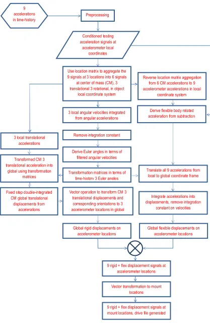
The drive file development process can be outlined using a flowchart, see Figure 4.2. A five-step

pro-cess describes the generation of the final displacement signals (drive file). This algorithm is programmed