Impacts of Ice Nucleation on Regional Climate and Air Quality Using WRF-CAM5: Application, Evaluation, and Sensitivity Study.

(1)

Zhang).

Aerosol particles serve as a source of ice nuclei (IN); they therefore, affect cloud

microphysical properties. However, large uncertainties exist in ice nucleation processes and

mechanisms. In order to investigate the impact of heterogeneous deposition/condensation ice

nucleation on air quality and climate modeling, the sensitivity of the model predictions to

different ice nucleation parameterizations is examined. In this study, the simulations using

the Weather Research and Forecasting model coupled with the physics and aerosol package

from the Community Atmosphere Model version 5 (WRF-CAM5) are conducted over the

East Asia for two full years (2006 and 2011), with two different heterogeneous

deposition/condensation ice nucleation schemes. The default scheme parameterization,

developed by Meyers et al. in 1992, only links the IN concentration to ice supersaturation,

whereas the new scheme of Niemand et al. (2012) parameterizes the IN concentration as a

function of temperature and dust surface areas. Comprehensive model performance

evaluations of the simulations with two different schemes for 2006 and 2011 are performed

using available satellite data, reanalysis data, and surface observations. The model shows a

comparable performance for meteorological variables at surface (i.e., temperature at 2 m

(T2), wind speed at 10 m (WS10), and radiation at ground), but large differences exist in

cloud variables and radiative forcing at top of the atmosphere (TOA), indicating large

uncertainties in cloud microphysics parameterizations. Significantly low biases exist in the

(2)

in CAM5.

The new scheme produces significantly higher IN concentrations in the northern

domain where dust source and downwind regions are located, leading to significantly higher

ice number concentrations in these regions, but significantly lower IN concentrations in the

southern domain. The larger IN concentrations lead to an increase in ice water path (IWP)

and a decrease in cloud liquid water path (CWP) caused by the enhancement of

Bergeron-Findeisen process in mixed-phase clouds. Despite the overall similar domainwide predictions

of IWP, CWP and cloud optical thickness (COT) for the two simulations with different ice

nucleation schemes, significant differences are found in their spatial distributions. Overall,

N12 gives relatively lower domainwide IWP and relatively larger CWP and COT. The

increase in COT results in a stronger shorwave radiation, longwave radiation, and cloud

forcing (net cooling) at top of atmosphere and a subsequent decrease in T2. The decreases in

T2 and radiation are associated with the decreases in mixing ratios of oxidants (i.e., OH and

O3) and mass concentrations of aerosol particles at surface (i.e., sulfate, PM2.5, and PM10).

Considerable improvements are found in the simulated CWP, COT, column SO2, and surface

mixing ratios of O3 in the simulations with the new ice nucleation scheme. Results of this

research provide information on the uncertainties of deposition and condensation ice

nucleation in WRF-CAM5 and identify regions that show increased sensitivity to the

(3)

(4)

by Ying Chen

A thesis submitted to the Graduate Faculty of North Carolina State University

in partial fulfillment of the requirements for the degree of

Master of Science

Marine, Earth, and Atmospheric Sciences

Raleigh, North Carolina

2015

APPROVED BY:

_______________________________ ______________________________

Dr. Yang Zhang Dr. Viney P. Aneja

Committee Chair

(5)

BIOGRAPHY

Ying Chen was born and raised in Haikou, China where from a young age she had

developed an interest in environmental protection. Upon graduating from high school in

2008, she entered Peking University to study Environmental Science. Her first research

experience was in the atmospheric chemistry research group in Peking University working

under her undergraduate advisor, Dr. Min Hu, where she assisted with the work on

atmospheric pollutant monitoring and composition analysis. After she graduated from Peking

University, she entered the M.S. Atmospheric Sciences program at NC State in fall 2012 and

worked on the regional atmospheric modeling over East Asia in Dr. Yang Zhang’s Air

(6)

ACKNOWLEDGMENTS

First, I would like to thank my committee members, Drs. Yang Zhang, Viney P.

Aneja, and Anantha R. Aiyyer. I am extremely grateful to Dr. Zhang for giving me the

opportunity to work on this project and giving me numerous opportunities for academic

growth throughout the entire process. I also greatly appreciate the scientific knowledge and

guidance provided by Drs. Viney P. Aneja and Anantha R. Aiyyer to take my M.S. research

to its full potential.

Second, I would like to thank collaborators from the Pacific Northwest National

Laboratory (PNNL), Drs. Jiwen Fan and Ruby Leung, for developing and implementing the

new ice nucleation scheme in the WRF-CAM5 model, members of Tsinghua University for

providing the emissions for 2006 and 2011. Thanks are due to the following people for their

scientific contributions: Dr. Kai Wang, Jian He, Xin Zhang, and Changjie Cai. I also wish to

thank the DOE climate modeling program (DE-SC000695) for supporting this research.

I wish to extend special thanks to all the members of the Air Quality Forecasting Lab

(past and present). Each has provided endless guidance and assistance in my research process

and even personal life.

Finally, I want to thank those people that served as my unwavering support system.

Enormous thanks are due to my parents, Chengfa and Yumei, and my brother, Wenpeng.

You have been behind me through everything and have given me endless support and

encouragement. To my boyfriend, Yizhou, and the future family, you have given me the

(7)

without you. To my friends in the US and China, thanks for your support through the hard

(8)

TABLE OF CONTENTS

LIST OF TABLES ... vii

LIST OF FIGURES ... ix

ACRONYMS ... xxv

CHAPTER 1. INTRODUCTION ... 1

1.1 Background and Motivations ... 1

1.2 Objectives ... 2

CHAPTER 2. LITERAUTRE REVIEW ... 4

2.1 Ice Nucleation and Its Climate Impacts ... 4

2.2 Mechanisms of Ice Nucleation ... 11

2.2.1 Heterogeneous Classical Nucleation Theory (CNT) ... 11

2.2.2 The Stochastic Description ... 14

2.2.3 The Singular Description ... 16

2.3 Sensitivity to Explicit Ice Nucleation Schemes ... 16

CHAPTER 3. DESCRIPTION OF MODEL, DATABASE, AND METHODOLOGY ... 23

3.1 Modeling System... 23

3.2 Episode Selection ... 28

3.3 Observational Networks ... 28

3.3.1 Meteorological Data... 29

3.3.2 Chemical Data ... 29

3.3.3 Satellite Data ... 30

3.4 Evaluation Protocols ... 32

3.4.1 Spatial Evaluation ... 32

3.4.2 Statistical Evaluation ... 32

3.4.3 Site Specific Evaluation ... 34

CHAPTER 4. EVALUATION OF BASELINE SIMULATION RESULTS ... 35

4.1 2006 Application and Evaluation ... 35

4.1.1 Meteorological Predictions ... 35

4.1.2 Chemical Predictions ... 65

(9)

4.2.1 Comparison of emissions in 2011 with in 2006... 95

4.2.2 Meteorological Predictions ... 99

4.2.3 Chemical Predictions ... 128

CHAPTER 5. SENSITIVITY TO EXPLICIT ICE NUCLEATION SCHEMES ... 142

5.1 Performance Evaluation ... 142

5.2 Sensitivity to Explicit Ice Nucleation Schemes ... 156

5.2.1 Spatial Comparison ... 156

5.2.2 Vertical Comparison ... 167

5.3 Examination of Ice Nucleation Indirect Climate Effects ... 175

5.3.1 Cloud Microphysical Effects ... 177

5.3.2 Radiative and Temperature Effects ... 202

5.3.3 Precipitation Effects ... 212

5.3.4 Chemical Effects ... 217

CHAPTER 6. SUMMARY AND CONCLUSIONS ... 227

(10)

LIST OF TABLES

Table 2.1 Comparison of major features of M92, N12, D10, P08, and C08 ... 22

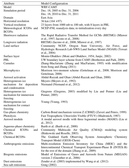
Table 3.1 Model configuration used in the WRF-CAM5 simulations ... 27

Table 3.2 Summary of observational networks ... 31

Table 4.1 Performance statistics for T2, Q2, WS10, P, and precipitation for 2006 ... 42

Table 4.2 Performance statistics for cloud parameters for 2006 ... 46

Table 4.3 Performance statistics for LWCF, and SWCF for 2006 ... 50

Table 4.4 Performance statistics for surface chemical species for 2006 ... 73

Table 4.5 Performance statistics for column chemical species for 2006 ... 78

Table 4.6 Comparison of annual emissions for 2006 and 2011 ... 96

Table 4.7 Performance statistics for T2, Q2, WS10, P, and precipitation for 2011 ... 103

Table 4.8 Performance statistics for cloud parameters for 2011 ... 107

Table 4.9 Performance statistics for LWCF, and SWCF for 2011 ... 111

Table 4.10 Performance statistics for surface chemical species for 2011 ... 133

Table 4.11 Performance statistics for column mass abundances of chemical species for ... 2011 ... 138

(11)

Table 5.2 Performance statistics for T2, P, Q2, WS10, precipitation, and radiation at …

surface for the 2011 simulation with N12 ... 148

Table 5.3 Performance statistics for cloud parameters for the 2006 simulation with N12 ... 150

Table 5.4 Performance statistics for cloud parameters for the 2011 simulation with N12 ... 152

Table 5.5 Performance statistics for column chemical species for the 2006 simulation …..

with N12 ... 154

Table 5.6 Performance statistics for column chemical species for the 2011 simulation …..

(12)

LIST OF FIGURES

Figure 2.1 Representation of different mechanisms of ice nucleation (Hoose et al., 2012) ... 7

Figure 2.2 Schematic diagram of warm cloud effects due to CCN (solid arrows) and …

glaciation effects due to IN (dash arrows) (Lohmann and Feichter, 2005). ... 10

Figure 2.3 Decay of liquid droplet with time for (a) single component model and (b) …

multiple component model (Murray et al., 2012) ... 15

Figure 3.1 modeling domain of WRF-CAM5 ... 26

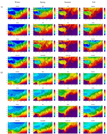
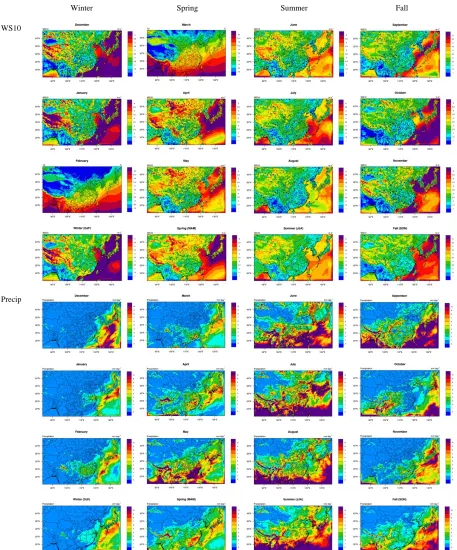
Figure 4.1 Spatial distributions of simulated monthly-average and seasonal-average T2 …

and Q2 overlaid with observations from NCDC. ... 51

Figure 4.2 Spatial distributions of simulated monthly-average and seasonal-average …..

WS10 and Precipitation overlaid with observations from NCDC. ... 52

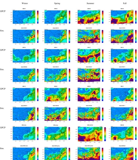
Figure 4.3 Comparison of simulated daily precipitation against GPCP for January, …

February, March, April, May, June, July, August, September, October, …

November, December, Winter, Spring, Summer, and Fall for 2006. ... 53

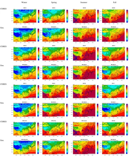
Figure 4.4 Comparison of simulated GLW against CERES for January, February, March, …

April, May, June, July, August, September, October, November, December, …

Winter, Spring, Summer, and Fall for 2006. ... 54

Figure 4.5 Comparison of simulated SWD against CERES for January, February, March, …

(13)

Figure 4.6 Comparison of simulated CCN against MODIS for January, February, March, …

Figure 4.7 Comparison of simulated CDNC in warm clouds against TERRA for January, …

Figure 4.8 Comparison of simulated CF against MODIS for January, February, March, …

Figure 4.9 Comparison of simulated CWP against MODIS for January, February, March, …

Figure 4.10 Comparison of simulated IWP against MODIS for January, February, March, …

Figure 4.11 Comparison of simulated PWV against MODIS for January, February, March, …

(14)

Figure 4.12 Comparison of simulated COT against MODIS for January, February, March, …

Figure 4.13 Comparison of simulated LWCF against CERES for January, February, …

March, April, May, June, July, August, September, October, November, …

December, Winter, Spring, Summer, and Fall for 2006. ... 63

Figure 4.14 Comparison of simulated SWCF against CERES for January, February, …

Figure 4.15 Simulated monthly-average and seasonal-average PM10 overlaid with ……..

API-derived PM10 from MEP China. ... 81

Figure 4.16 Comparisons of simulated and observed monthly-average and seasonal-average

mixing ratios of CO at surface over Taiwan, Japan, and South Korea. ... 82

Figure 4.17 Comparisons of simulated and observed monthly-average and seasonal-…

average mixing ratios of NO at surface over Taiwan, Japan, and South …

Korea. ... 83

average mixing ratios of NO2 at surface over Taiwan, Japan, and South …

(15)

average mixing ratios of NO2 and SO2 at surface over Taiwan, Japan, and …

South Korea. ... 85

average mixing ratios of O3 at surface over Taiwan, Japan, and South …..

Korea. ... 86

average mixing ratios of O3 and PM2.5 at surface over Taiwan, Japan, and …

South Korea. ... 87

Figure 4.22 Comparisons of simulated and observed monthly-average and seasonal-….

average mass concentrations of PM10 at surface over Mainland China, Hong …

Kong, Taiwan, Japan, and South Korea. ... 88

Figure 4.23 Comparisons of simulated and observed seasonal-average and annual-….

average mass concentrations of PM2.5 and its compositions at THU and …

Miyun. ... 89

Figure 4.24 Comparison of simulated column CO against MOPPIT for January, February, …

(16)

Figure 4.25 Comparison of simulated column NO2 against SCIAMACHY for January, …

Figure 4.26 Comparison of simulated column SO2 against SCIAMACHY for January, …

Figure 4.27 Comparison of simulated column TOR against OMI for January, February, …

Figure 4.28 Comparison of simulated AOD against MODIS for January, February, March, …

Figure 4.29 Comparisons of emissions of major gasous species in 2011 with those in ….

2006. ... 97

Figure 4.30 Comparisons of emissions of major aerosol species in 2011 with those in …

2006. ... 98

Figure 4.31 Spatial distributions of simulated seasonal-average and annual-average T2 …

overlaid with observations from NCDC and absolute and percentage …

(17)

Figure 4.32 Spatial distributions of simulated seasonal-average and annual-average Q2 …

differences for 2011. ... 113

Figure 4.33 Spatial distributions of simulated seasonal-average and annual-average WS10 …

differences for 2011. ... 114

Figure 4.34 Spatial distributions of simulated seasonal-average and annual-average PBLH …

and absolute and percentage differences for 2011. ... 115

Figure 4.35 Spatial distributions of simulated seasonal-average and annual-average …

precipitation overlaid with observations from NCDC and absolute and …

percentage differences for 2011. ... 116

Figure 4.36 Spatial distributions of simulated seasonal-average and annual-average SWD …

Figure 4.37 Spatial distributions of simulated seasonal-average and annual-average GLW …

Figure 4.38 Spatial distributions of simulated seasonal-average and annual-average CCN …

Figure 4.39 Spatial distributions of simulated seasonal-average and annual-average CDNC ...

(18)

Figure 4.40 Spatial distributions of simulated seasonal-average and annual-average CF ……

and absolute and percentage differences for 2011...………121

Figure 4.41 Spatial distributions of simulated seasonal-average and annual-average CWP …

and absolute and percentage differences for 2011 ... 122

Figure 4.42 Spatial distributions of simulated seasonal-average and annual-average IWP ….

Figure 4.43 Spatial distributions of simulated seasonal-average and annual-average PWV ….

Figure 4.44 Spatial distributions of simulated seasonal-average and annual-average COT …

Figure 4.45 Spatial distributions of simulated seasonal-average and annual-average LWCF ..

Figure 4.46 Spatial distributions of simulated seasonal-average and annual-average SWCF …

Figure 4.47 Simulated monthly-average and seasonal-average PM10 overlaid with ……..

API-derived PM10 from MEP China....………141

Figure 5.1 Spatial distributions of IND simulated by M92 and N12 for monthly-mean …

and seasonal-mean in 2006 ... 159

Figure 5.2 Spatial distributions of INT simulated by M92 and N12 for monthly-mean and ….

(19)

Figure 5.3 Comparison of month variation of domainwide average INM (top left), INT ….

(top right), IND (bottom left), and CINC (bottom right) simulated by N12 and …

M92 ... 161

Figure 5.4 Spatial distributions of CINC simulated by M92 and N12 for monthly-mean ….

and seasonal-mean in 2006 ... 162

Figure 5.5 Absolute (top) and percentage (bottom) differences for CINC between N12 and …

M92 for 2006 in monthly-mean for (a) January, (b) February, and (c) …

December, and (d) in seasonal-mean for winter ... 163

M92 for 2006 in monthly-mean for (a) March, (b) April, and (c) May, and (d) …

in seasonal-mean for spring ... 164

M92 for 2006 in monthly-mean for (a) June, (b) July, and (c) August, and (d) …

in seasonal-mean for summer ... 165

M92 for 2006 in monthly-mean for (a) September, (b) October, and (c) …

November, and (d) in seasonal-mean for fall ... 166

Figure 5.9 The vertical distributions for IND for M92 and N12 monthly-mean for (a) …

January, (b) February, (c) March, (d) April, (e) May, (f) June, (g) July, (h) …

(20)

seasonal-mean for (m) winter, (n) spring, (o) summer, and (p) fall, and (q) in …

annual-mean in 2006 ... Error! Bookmark not defined.

Figure 5.10 The vertical distributions for CINC for M92 and N12 monthly-mean for (a) …

January, (b) February, (c) March, (d) April, (e) May, (f) June, (g) July, (h) …

August, (i) September, (j) October, (k) November, and (l) December, in …

seasonal-mean for (m) winter, (n) spring, (o) summer, and (p) fall, and (q) in …

annual-mean in 2006 ... Error! Bookmark not defined.

Figure 5.11 Schematic diagram of the effects of the change of IND on cloud properties, …

radiation, precipitation, temperature, and chemical species, and the feedback …

of them ... 176

Figure 5.12 Spatial comparison of column total IWP from reanalysis data from MODIS …

(column 1), M92 (column 2) and N12 (column 3) for monthly-mean of …

January (row 1), February (row 2), and December (row 3), and seasonal-mean ..

of winter (row 4) in 2006 ... 182

March (row 1), April (row 2), and May (row 3), and seasonal-mean of spring …

(row 4) in 2006 ... 183

(21)

(row 1), July (row 2), and August (row 3), and seasonal-mean of summer …

(row 4) in 2006 ... 184

September (row 1), October (row 2), and November (row 3), and seasonal-…

mean of fall (row 4) in 2006 ... 185

Figure 5.16 The vertical distributions for ice mixing ratios due to cloud ice for M92 and …

N12 monthly-mean for (a) January, (b) February, (c) March, (d) April, (e) …

May, (f) June, (g) July, (h) August, (i) September, (j) October, (k) ….

November, and (l) December, in seasonal-mean for (m) winter, (n) spring, …

(o) summer, and (p) fall, and (q) in annual-mean in 2006Error! Bookmark not defined.

Figure 5.17 A schematic diagram depicting the cloud and precipitation processes in CAM …

(Rutledge and Hobbs, 1984) ... 189

Figure 5.18 Absolute and percentage differences for IWP due to ice (column 1), IWP due …

to snow (column 2), and IWP due to ice and snow (column 3) between N12 …

and M92 for 2006 in monthly-mean for (a) January, (b) February, and (c) …

December, and (d) in seasonal-mean for winter ... 190

(22)

and M92 for 2006 in monthly-mean for (a) March, (b) April, and (c) May, and …

(d) in seasonal-mean for spring ... 191

and M92 for 2006 in monthly-mean for (a) June, (b) July, and (c) August, and …

(d) in seasonal-mean for summer ... 192

and M92 for 2006 in monthly-mean for (a) September, (b) October, and (c) ….

November, and (d) in seasonal-mean for fall ... 193

Figure 5.22 Absolute and percentage differences for CWP due to QCLOUD (column 1), …

CWP due to QRAIN (column 2), and CWP due to QCLOUD and QRAIN …

(column 3) between N12 and M92 for 2006 in monthly-mean for (a) January, …

(b) February, and (c) December, and (d) in seasonal-mean for winter ... 194

(column 3) between N12 and M92 for 2006 in monthly-mean for (a) March, …

(b) April, and (c) May, and (d) in seasonal-mean for spring ... 195

(23)

(column 3) between N12 and M92 for 2006 in monthly-mean for (a) June, ……

(b) July, and (c) August, and (d) in seasonal-mean for summer ... 196

(column 3) between N12 and M92 for 2006 in monthly-mean for (a) …

September, (b) October, and (c) November, and (d) in seasonal-mean for ……

fall ... 197

Figure 5.26 Absolute and percentage differences for COT (column 1), PWV (column 2), …

and CF (column 3) between N12 and M92 for 2006 in monthly-mean for (a) …

January, (b) February, and (c) December, and (d) in seasonal-mean for …...

winter. ... 198

March, (b) April, and (c) May, and (d) in seasonal-mean for spring ... 199

June, (b) July, and (c) August, and (d) in seasonal-mean for summer ... 200

(24)

fall ... 201

Figure 5.30 Absolute and percentage differences for SWCF (column 1), LWCF ……..

(column 2), and T2 (column 3) between N12 and M92 for 2006 in monthly-…

mean for (a) January, (b) February, and (c) December, and (d) in seasonal-…

mean for winter. ... 204

Figure 5.31 Absolute and percentage differences for SWCF (column 1), LWCF ……..

mean for (a) March, (b) April, and (c) May, and (d) in seasonal-mean for …

spring ... 205

Figure 5.32 Absolute and percentage differences for SWCF (column 1), LWCF …….

mean for (a) June, (b) July, and (c) August, and (d) in seasonal-mean for …

summer ... 206

Figure 5.33 Absolute and percentage differences for SWCF (column 1), LWCF …….

mean for (a) September, (b) October, and (c) November, and (d) in seasonal-…

mean for fall ... 207

Figure 5.34 Absolute and percentage differences for SWD (column 1), OLR (column 2), …

(25)

January, (b) February, and (c) December, and (d) in seasonal-mean for …..

winter ... 208

and LH (column 3) between N12 and M92 for 2006 in monthly-mean for (a) …

March, (b) April, and (c) May, and (d) in seasonal-mean for spring ... 209

June, (b) July, and (c) August, and (d) in seasonal-mean for summer ... 210

fall ... 211

Figure 5.38 Absolute (top) and percentage (bottom) differences for precipitation between …

N12 and M92 for 2006 in monthly-mean for (a) January, (b) February, and (c) …

December, and (d) in seasonal-mean for winter. ... 213

N12 and M92 for 2006 in monthly-mean for (a) March, (b) April, and (c) ….

(26)

N12 and M92 for 2006 in monthly-mean for (a) June, (b) July, and (c) ….

August, and (d) in seasonal-mean for summer ... 215

N12 and M92 for 2006 in monthly-mean for (a) September, (b) October, and …

(c) November, and (d) in seasonal-mean for fall ... 216

Figure 5.42 Absolute and percentage differences for mixing ratios of surface OH ……

(column 1) and O3 (column 2) between N12 and M92 for 2006 in monthly-…

mean for (a) January, (b) February, and (c) December, and (d) in seasonal-…

mean for winter ... 219

mean for (a) March, (b) April, and (c) May, and (d) in seasonal-mean for …

spring ... 220

mean for (a) June, (b) July, and (c) August, and (d) in seasonal-mean for …

summer ... 221

(27)

mean for (a) September, (b) October, and (c) November, and (d) in seasonal-…

mean for fall ... 222

Figure 5.46 Absolute and percentage differences for mass concentrations of PM10 …..

(column 1), PM2.5 (column 2), and sulfate (column 3) between N12 and M92 …

for 2006 in monthly-mean for (a) January, (b) February, and (c) December, …

and (d) in seasonal-mean for winter ... 223

Figure 5.47 Absolute and percentage differences for PM10 (column 1), PM2.5 (column 2), …

and sulfate (column 3) between N12 and M92 for 2006 in monthly-mean for …

(a) March, (b) April, and (c) May, and (d) in seasonal-mean for spring ... 224

Figure 5.48 Absolute and percentage differences for PM10 (column 1), PM2.5 (column 2), …

(a) June, (b) July, and (c) August, and (d) in seasonal-mean for summe ... 225

Figure 5.49 Absolute and percentage differences for PM10 (column 1), PM2.5 (column 2),…

(a) September, (b) October, and (c) November, and (d) in seasonal-mean for …

(28)

ACRONYMS

Acronym Definition

α –PDF Probability-density-function-of-α (contact angle) Model

AOD Aerosol Optical Depth

API Air Pollution Index

AQMN Air Quality Monitoring Network

BC Black Carbon

BCON Boundary Conditions

C08 Ice Nucleation Scheme Developed by Chen et al. (2008)

CAM3 The Community Atmospheric Model Version 3

CAM5 The Community Atmospheric Model Version 5

CAPE Consumption of Convective Available Potential Energy

CBMZ Carbon-Bond Mechanism Version Z

CCN Cloud Condensation Nuclei

CDNC Cloud Droplet Number Concentration

CERES Clouds and The Earth’s Radiant Energy System

CF Cloud Fraction

CINC Cloud Ice Number Concentration

CMAQ The Community Multiscale Air Quality Modeling System

CNT Classical Nucleation Theory

CO Carbon Monoxide

(29)

CWP Cloud Liquid Water Path

D10 Ice Nucleation Scheme Developed by Demott et al. (2010)

DM Dust/Metallic Aerosols

EPD Environmental Protection Department

FTUV Fast Tropospheric Ultraviolet-Visible Scheme

GCMs The Global Climate Models

GEOS-Chem Goddard Earth Observing System Atmospheric Chemistry Transport Model

GLW Downward Longwave Flux At Surface

GPCP Global Precipitation Climatology Project

HCHO Formaldehyde

HUCM Hebrew University Spectral Microphysics Cloud Model

ICON Initial Conditions

IN Ice Nuclei

INTEX-B Intercontinental Chemical Transport Experiment-Phase B

IP Ice Particle

IWP Cloud Ice Water Path

L07 Ice Nucleation Scheme Developed by Liu et al. (2007)

LH Latent Heat

IND IN due to Deposition/Condensation Nucleation

INM IN Due to Immersion Freezing

INT Total IN

(30)

LWCF Longwave Cloud Forcing at TOA

LTS Lower-tropospheric Stability

M92 Ice Nucleation Scheme Developed by Meyers et al. (1992)

MAM The Modal Aerosol Module of Liu et al. (2012)

MB Mean Bias

MEGAN2 The Model Of Emissions Of Gases and Aerosols From Nature Version 2

MEIC The Multi-Resolution Emission Inventory for China

MEP Ministry of Environmental Protection

MODIS Moderate Resolution Imaging Spectroradiometer

MOPITT Measurements of Pollution in The Troposphere

N12 Ice Nucleation Scheme Developed by Niemand et al. (2012)

NASA National Atmospheric and Space Administration

NCAR National Center for Atmospheric Research

NCDC The National Climatic Data Center

NCEP The National Centers for Environmental Prediction

NH3 Ammonia

NH4+ Ammonium

NIES National Institute of Environmental Studies

NMB Normalized Mean Bias

NME Normalized Mean Error

NO Nitrogen Monoxide

(31)

NO3- Nitrate

NOAA The National Oceanic and Atmospheric Administration

NOAH The NCEP, Oregon State University, Air Force, and Hydrologic Research

Lab’s

O3 Ozone

OC Organic Carbon

OH Hydroxyl Radical

OMI Ozone Monitoring Instrument

P Air Pressure

P08 Ice Nucleation Scheme Developed by Phillips et al. (2008)

PBL Planet Boundary Layer

PBLH PBL Height

PM Particulate Matter

PM10 Particulate Matter with Diameter less than or equal to 10 µm

PM2.5 Particulate Matter with Diameter less than or equal to 2.5 µm

PNNL The Pacific Northwest National Laboratory

PRD The Pearl River Delta

PWV Precipitable Water Vapor

Q2 Water Vapor Mixing Ratios at 2 Meters

R Correlation Coefficient

RH Relative Humidity

RMSE Root Mean Square Error

(32)

S Supersaturation

SCIAMACHY The Scanning Imaging Absorption Spectrometer for Atmospheric Chartography

SO2 Sulfur Dioxide

SO42- Sulfate

SOA Secondary Organic Aerosols

SNA Sulfate, Nitrate, and Ammonium

SWCF Shortwave Cloud Forcing at TOA

SWD Downward Shortwave Flux at Ground Surface

T Temperature

t Time

T2 Temperature at 2 Meters

THU Tsinghua University, China

TOA Top of Atmosphere

TOR Tropospheric Ozone Residual

UW University of Washington

VOC Volatile Organic Carbon

WRF-CAM5 The Weather Research and Forecasting Model with the Physics Package

from CAM5

(33)

CHAPTER1. INTRODUCTION

1.1 Background and Motivations

Clouds are ubiquitous in the troposphere and control the Earth’s radiative forcing by

interacting with both incoming shortwave and outgoing longwave radiation (Lohmann and

Feichter, 2005). The formation of ice particles, which is an important process in both ice

cloud, like cirrus cloud and mixed cloud, like orographic cloud, play an important role in the

climate system via changing the microphysical properties of clouds and initiating

precipitation. Aerosols are reported to act as ice nuclei (IN) to catalyze the formation of ice

particles in clouds. Such aerosol-ice-cloud interaction on climate is called “ice indirect

effect” or “glaciation indirect effect” (Lohmann, 2002). Although the aerosol-cloud

interaction represents one of the largest uncertainties in current modulating climate (Solomon

et al., 2007), the uncertainty of “ice indirect effect”, especially such effects in mixed-phase

clouds are even acute.

Ice nucleation is depicted to increase the number concentration of ice crystals in the

cloud, initiate and increase precipitation, and reduce cloud lifetime, therefore has a positive

effect on climate radiative forcing. However, the impacts of ice nucleation on the global

climate are unquantified, because of lacking of comprehensive understanding of the

mechanism of ice nucleation and the relationship between ice nucleation and the change of

cloud properties. The glaciation temperature and supersaturation for ice nucleation are

(34)

materials, represent one of the largest difficulties in describing their ability crystalizing ice

particles in models (Murray et al., 2012).

Several reviews of ice nucleation have covered the findings in terms of the

mechanisms (Martin, 2000; Murray et al., 2012; Barahona, 2012), the effects on climate

(Wisniewski et al., 1997), field (Martin, 2000) and laboratory results (Hoose and Mohler,

2012), and modeling work of ice nucleation. To reduce the complicity of calculating ice

nucleation in the model, several parameterizations have been implemented in numerical

models. These parameterizations are based on lab or field results (Meyers et al., 1992;

Phillips et al., 2008; DeMott et al., 2010; Niemand et al., 2012), or the combination of both

lab results and classical nucleation theory (Liu and Penner, 2005; Chen et al., 2008). Since

ice cloud formation is sensitive to the treatment of ice nucleation in the model, it would be

useful to compare different ice nucleation schemes.

Giving the importance of ice nucleation on climate and the lack of understanding of

its mechanisms, the goal of this study is to analyze the sensitivity of simulated microphysical

processes and their feedbacks on cloud properties to different treatments of ice nucleation.

1.2 Objectives

In this study, the Weather Research and Forecasting model with the physics package

from the National Center for Atmospheric Research's Community Atmospheric model

version 5 (CAM5) (i.e., WRF-CAM5) is applied to simulate meteorology, air quality, and

(35)

(1) Evaluate the updated WRF-CAM5’s capability in simulating meteorological and

chemical variables;

(2) Examine the sensitivity of model predictions to different heterogeneous ice nucleation

(36)

CHAPTER 2. LITERAUTRE REVIEW

2.1 Ice Nucleation and Its Climate Impacts

Clouds are vital in the Earth’s atmosphere. Clouds modify the radiation budget by

reflecting incoming shortwave radiation and absorbing outgoing longwave radiation (IPCC

Fourth Assessment Report, 2013). Clouds reflect solar radiation back to space, cooling the

planet. However, these clouds, being cool, lead to weakened surface cooling, according to

Kirchhoff’s law (Kirchhoff, 1860). The balance of these two processes determines the net

cloud radiation forcing (Hartmann et al., 1992; Ockert-Bell and Hartmann, 1992). In

addition, as an integral part of the hydrological cycle, clouds indirectly control the climate

via its responsibility for water transport and precipitation. Cloud net climate effects are

driven by cloud properties, such as types of clouds, cloud water content, albedo, lifetime,

cloud droplet sizes and radiative properties (Lohmann and Feichter, 2005).

Tropospheric clouds can be classified into two broad categories: glaciated (cirrus)

cloud and mixed-phase clouds. Cirrus clouds, which consist of entirely ice, play an important

role in climate (Liou, 1986), water transport (Holton and Gettelman, 2001), and numerous

chemical processes (Abbatt, 2003). Mixed-phase clouds, existing in the low and middle

troposphere at temperatures between around 237 K and 273 K, are usually composed of both

ice particles and supercool water droplets. Mixed-phase clouds include cumulus, stratus, and

(37)

influence on radiation forcing and energy budget (Curry, 1995; Morrison et al., 2012). Ice

crystals exist in both types of clouds and exert an influence on climate.

Ice formation in clouds impacts the climate via three ways: 1) substantially

determines the cloud water content and affects the properties of clouds and their impacts on

the climate (Lohmann and Feichter, 2005); 2) releases a large amount of latent heat and

warms the clouds when super-cooled liquid water condenses on the surface of ice nuclei; 3)

potentially alters the energy and hydrological cycles by one of the key processes initiating

precipitation—ice crystals in the cloud (Lohmann, 2002).

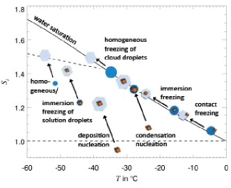
Ice nucleation in troposphere occurs via two pathways: homogeneous and

heterogeneous nucleation (Hallett and Mossop, 1974). Homogeneous nucleation occurs when

the temperature is below -35℃ and water droplet contains no foreign particles. Water

droplets can freeze in the presence of IN when the temperature is below 0 ℃ by

heterogeneous nucleation. Observations indicate that heterogeneous freezing is a

predominant mechanism for lower energy barrier and supersaturations to crystallization. The

homogeneous freezing threshold for pure cloud droplets to begin crystallizing is around 237

K while heterogeneous nucleation can catalyze freezing at warmer temperatures. There are a

number of ways in which heterogeneous ice nucleation are thought to occur. These include:

(1) deposition ice nucleation, during which water directly deposits from the vapor phase to a

solid surface as ice; (2) immersion freezing, during which a solid particle is immersed in the

supercooled liquid; (3) condensation freezing, during which water vapor condenses and then

(38)

a solid particle to induce freezing (Vali, 1985). Both deposition freezing and condensation

freezing require conditions exceeding water supersaturation at freezing temperatures. The

distinction of deposition freezing and condensation freezing is difficult. Different

mechanisms of different ice nucleation are depicted in Fig. 2.1. Once ice crystal is formed,

ice crystals may begin to grow by aggregation and accretion rapidly from preexisting ice

particles. While cirrus clouds typically form from supercool water droplets in the upper

troposphere via homogeneous or heterogeneous freezing, mixed-phase clouds can glaciate at

(39)

(40)

Unlike CCN, IN are solid, insoluble, and large particles with good nucleability, such

as mineral dust (Isono et al., 1959), clay minerals (Zuberi et al., 2002), soot (Kanji and

Abbatt, 2006), and carborneous particles (Diehl et al., 2001; DeMott et al., 2009). Such

particles will lose the ability to act as IN if sulfur dioxide (SO2), nitrite dioxide (NO2) or

ammonia (NH3) condense on their surfaces to form secondary aerosol. Aerosol particles are

considered as the major source of IN to form ice particles. However, only a small fraction of

aerosol particles in the atmosphere can be activated as IN, with activated fraction ranging

from 10-8 to 0.01 (Hoose and Mohlerr, 2012). The probabilities of different types of aerosol

particles to serve as IN have been investigated in numerous laboratory studies and field

campaigns (Hoose and Mohler, 2012). DeMott et al. (2003) indicated that the long-range

transported dust particles from North Africa contributed to the change of cloud properties

over Florida. Such a linkage has been found for Asian dust as well as Saharan dust (Mohler

et al., 2006; Niemand et al., 2012).

In the latest report of the Intergovernmental Panel on Climate Change (IPCC, 2013),

the estimation of the cloud radiative forcing of aerosol through ice nucleation is unable to be

determined. The studies of the climatic impacts of ice nucleation on both cirrus cloud and

mixed-phase clouds are limited and in their infantry. While there are large uncertainties in

terms of the indirect effects of aerosol on clouds, the effects of ice nucleation on climate via

clouds are even less understood. Most of the recent studies investigated the impacts of ice

nucleation as a part of the impacts of aerosol-cloud interaction. Since aerosol particles can

(41)

liquid droplets and increase the cloud droplet number concentration (CDNC), the impacts of

aerosol on clouds are the results of the competition between the cloud sensitivity to IN and

CCN (Fig. 2.2). Rosenfeld et al. (2011) showed convective clouds forming with small droplet

sizes (10-15 µm) and low glaciation temperature (-33 °C) in a smoke plume over China. In

this scenario, aerosol particles served as CCN instead of IN, leading to a substantial increase

of CCN number concentration and changes in the ratio of CCN to IN. The increase of overall

CCN led to more, but smaller cloud droplets to a decrease in precipitation and an increase of

cloud lifetime via the warm rain processes. Lohmann (2002a) pointed out a negative

feedback loop for the aerosol effects on mixed-phase clouds. Since soot particles can act as

IN, leading to the enhancement in terms of precipitation via ice formation, aerosols will be

removed from the atmosphere. The reduction of anthropogenic aerosol burden varies from

38% to 58%. Lohmann and Diehl (2006) demonstrated that ice nucleation enhanced

precipitation, which resulted in a substantial reduction of the lifetime of clouds, therefore led

to a warming effect on climate by exploring the impacts of dust and soot particles as IN in

mixed-phase clouds. The radiative forcing was sensitive to mineral dust and ranging from 1

to 2.1 W m-2. Such impacts have counteracted the cooling effects of increased CCN

influencing warm clouds, and similar results were obtained in other studies (Storelvmo et al.,

2008; Hoose et al., 2008). Although the increase of IN leads to more precipitation, but a short

cloud lifetime, Khain et al. (2008) found that the increase of IN might not lead to an increase

of precipitation. In addition, the sign and magnitude of the effects of ice nucleation in the

(42)

Figure 2.2 Schematic diagram of warm cloud effects due to CCN (solid arrows) and

glaciation effects due to IN (dash arrows) (Lohmann and Feichter, 2005).

In summary, the climate impacts of ice nucleation are complex and the related studies

are limited. There is a severe limitation in our understanding of ice nucleation, such as

quantitative understanding of the mechanisms of ice nucleation, especially the heterogeneous

ice nucleation in the presence of atmospheric aerosol, quantification of the changes to clouds

(43)

2.2 Mechanisms of Ice Nucleation

Substantial challenges remain in ice nucleation research. Different from cloud

droplets, the shapes of ice crystals are not unique, which increase the difficulty to describe

the diameter and shape of ice crystals in the model. Mineral and soil dust, carbonaceous

particles from fossil fuel combustion and biomass burning, crystallized salts, and pure

substances can act as IN. However, the temperatures at which various substances nucleate ice

vary from Cinnabar at -16℃ to pure ice crystal at 0 ℃. Aerosols can serve as heterogeneous

IN and hence are responsible for climate change by altering the microphysical properties of

cloud and initiating precipitation, which is called “cloud indirect effect”. The efficiency of

aerosol particles to act as heterogeneous IN depends on not only their chemical composition

but also their surface properties. The laboratory results of DeMott in 1990 showed that at

temperature below -25℃, soot particles can serve as IN. Carbonaceous particles (Chen et al.,

1998) and various crustal particles (Heintzenberg et al., 1996; Targiono et al., 2006),

especially dust particles have been found as the most abundant types of IN (Prenni et al.,

2007). To describe ice nucleation in the atmosphere, a classical nucleation theory of ice

nucleation is developed.

2.2.1 Heterogeneous Classical Nucleation Theory (CNT)

Classical nucleation theory is widely applied in calculating and representing

nucleation where a new phase nucleates from the pre-existing metastable phase (Kashchiev,

(44)

observed trends through estimating the rate of nucleation based on readily available

macroscopic quantities (Murray et al., 2010). The heterogeneous CNT is adopted from the

one for homogeneous nucleation. The rate coefficient 𝐽_ℎ𝑒𝑒 (cm-2 s-1) at which ice starts to

crystallize is associated to the Gibbs energy, which is required for a critical cluster forming in

an Arrhenius form (Arrhenius, 1889):

𝐽_ℎ𝑒𝑒(𝑇) =𝐴_ℎ𝑒𝑒 exp(−∆𝐺∗𝜑

𝑘𝑘 ) (2.1)

where ∆𝐺∗is the Gibbs free energy of forming a cluster, 𝑘 is the Boltzmann constant, T is the

temperature in K, 𝐴_ℎ𝑒𝑒 is a pre-exponential factor in units of cm-2s-1, φ is a factor, which can

reduce the required energy barrier to homogeneous nucleation in the presence of a solid and

can be descripted as a function of an ice nucleating efficiency parameter, m:

2

(2 m)(1 m) 4

ϕ = + − (2.2)

The ice nucleating efficiency parameter 𝑚 can be expressed as cos θ, where θ is defined as

the contact angle that a flat surface in contact with a spherical ice nucleus. However, the

values of θ vary by the shape and materials of IN. The Gibbs energy can be written:

3 2 *

2

16

3( ln )

G

kT S

πγ n

(45)

where γ is the surface tension (surface forming energy), n is the molecular volume of the

condensed phase, and S is the supersaturation. Combining (2.1), (2.2), and (2.3), the

heterogeneous nucleation rate can be expressed as:

3 2 2

3 3 2

16 (2 m)(1 m)

ln ln

3 (ln ) 4

het

J A

k T S

πγ n + −

= −

(2.4)

Multiple assumptions are needed to make to fit equation (2.4) to experimental data. In

order to describe heterogeneous CNT, two primary methods are developed: stochastic

approach and singular approach (Pruppacher and Klett, 1997). The stochastic approach

describes heterogeneous ice nucleation based on a fundamental understanding, whereas the

singular approach develops a relatively simple way to describe heterogeneous ice nucleation

by the major ice nucleating properties of aerosol particles. Ice nucleation is dependent on

both time and the amount of IN, which is clearly described in CNT. The nucleating

probabilities are considered to be identical in some idealized laboratory experiments to

diagnose the stochastic behavior of ice nucleation. However, since aerosol particles are

different in terms of the composition, shape and size, the effects of aerosol particles on

heterogeneous ice nucleation tend to be complex. To simplify the complex behavior of ice

nucleation, a singular approach was proposed by neglecting the stochastic behavior. Hence,

IN is assumed to form an ice germ as soon as the temperature reaches the freezing point,

(46)

2.2.2 The Stochastic Description

In the single component stochastic approach, the nucleation rate R can be defined as:

R dN J sN_het dt

= = − (2.5)

Where dN is number of ice activated in time t, and s is the nucleant surface area for dN.

Integrating (2.5), the fraction of droplets frozen can be expressed as a function of time:

1

1 exp( )

ice

het n

J s t N

∆ _{= −} ₋ _∆

(2.6)

where ∆𝑛_𝑖𝑖𝑒 is the number of droplets which freeze in a time increment (∆𝑡), and 𝑁₁ is the

number of ice crystals before ∆𝑡. However, the single-contact-angle (θ) model is implied to

be inadequate to describe the process of ice nucleation (Niedermeier et al., 2011; Murray et

al., 2011). Kulkarni et al. (2012) also ascribed the great differences for simulated cloud

properties due to the width of distribution of θ.

Overcoming the disadvantage of single component stochastic approach, multiple

component stochastic approach has been developed by summing the effects of different type

of ice nucleating particles. Similar to the single component stochastic approach, the fraction

of new-activated frozen droplets in ∆𝑡 can be expressed as:

1

1 exp( )

n ice

i i i n

J s t

N =

∆ _{= −} ₋ _∆

(47)

where J_i and s_i are the temperature dependent nucleation rate coefficient and surface area,

respectively, for each ice nucleus of type i. In the multiple-stochastic approach, the ice

crystal number concentration at a given time can be calculated if the composition of aerosol

particles and the contact angle for each component is known. In a recent model study, a

probability-density-function-of-α (α –PDF) model, which uses a probability density function

of contact angles instead of single values, shows better agreement with observations in

mixed-phase clouds, with more predicted ice crystals and weaker temperature dependence,

compared to the single-contact-angle model (Wang et al., 2014).

Figure 2.3 Decay of liquid droplet with time for (a) single component model and (b) multiple

(48)

2.2.3 The Singular Description

The singular approach is based on the assumption that the stochastic behavior of

nucleation is less important than the distribution of IN types. Thus, immersion freezing by a

certain IN type cannot occur if the temperature is above a characteristic temperature, T, based

on the assumption of singular approach. The fraction of frozen droplets at temperature T, f_ice

, can be expressed as:

( ) ice( ) 1 exp( ( ) )

ice s

tot

n T

f T n T s

N

= = − − (2.8)

where 𝑛𝑖𝑖𝑒(𝑇) is the cumulative number of frozen droplets at temperature T, N_tot is total

number for frozen droplets, n Ts( ) is the cumulative number of nucleation sites per surface

area, and s is the nucleant surface area. Several empirical expressions (Meyers et al., 1992;

Phillips et al., 2008; DeMott et al., 2010; Niemand et al., 2012) based on freezing events

have been developed and imply a singular, time-independent ice nucleation.

2.3 Sensitivity to Explicit Ice Nucleation Schemes

Despite the importance of ice nucleation, the treatment of ice nucleation in current

numerical models is not explicit for lack of comprehensive understanding of the mechanisms

of ice nucleation and in-situ observations. To improve the prediction of ice crystal number

concentrations in numerical models, various ice nucleation schemes have been developed. To

(49)

parameterizations to calculate ice nucleation based on fitting the observed ice crystal number

concentration to temperature and/or ambient supersaturation. For instance, Meyers et al.

(1992) predicted the number of ice crystals due to deposition-condensation freezing (Nid) by

the parameterization

N_id =exp( 0.639 0.1296(100(− + S_i−1))) (2.9)

where (Si -1) is the fractional ice supersaturation. Such formulation is widely used in

numerical models, such as CAM3 (DeMontt et al., 2010), CAM5 (Xie et al., 2013; English et

al., 2014), and the Hebrew University spectral microphysics cloud model (HUCM) (Khain et

al., 2008). However, the formulation is empirical and based on very limited field studies at

northern midlatitudes and may be applied over the temperature range from -7 to -20°C, ice

supersaturation range from 2% to 25%, and water supersaturation range from -5% to 4.5%.

To improve the prediction of ice crystal number concentration, the temporal and spatial

variability of IN are taken into account. Ice nuclei, generally are insoluble aerosol particles

such as dust, soot, and carbonaceous particles, are treated explicitly based on aerosol

properties.

Niemand et al. (2012) (N12) proposed a new parameterization based on the crucial

role of dust particle in condensation freezing and cloud chamber experiments. In Niemand’s

parameterization, ice crystal number concentration is a function of temperature, ambient

(50)

N_{i j}_, =N_{tot j}_, (1 exp( S− − _{ae j}_, n T_s( )) (2.10)

n T_s( )=exp( 0.517(T 273.15) 8.934)− − + (2.11)

where Ni,j is the number of active IN in size bin j, Ntot,j is the total number of particles in size

bin j and Sae,j is the individual particle surface area in that size bin. The density of ice-active

surface sites ns(T) is calculated based on a temperature-dependent fit to observational studies.

The valid temperature range for Niemand parameterization is -12° and -36°C.

Similarly, DeMott et al. (2010)(D10) introduced a parameterization that ice crystal

number concentration is associated with temperature and aerosol particles based on nine

separate field studies conducted over a 14-year period in many locations of the globe. The ice

nuclei number concentration at Tk (cloud temperature in degree Kelvin), nIN T,_k, is given by:

_, (273.16 ) ( _,0.5)( (273.16 k) ) k

c T d b

IN T k aer

n =a −T n − + (2.12)

where a = 5.94 10× −5, b = 3.33, c = 0.0264, d = 0.0033, and n_aer_,0.5 (cm-3) is the number

concentration of aerosol particles with diameters larger than 0.5 µm. Xie et al. (2013)

compared DeMott’s scheme with Meyers’s scheme and found that DeMott’s scheme slightly

improved low-level cloud simulation over the Arctic but worsened in predicting mid-level

clouds.

An ice nucleation parameterization (Phillips et al. 2008) (P08) that fits IN

(51)

types of aerosol particles, such as dust/metallic aerosols (DM), soot particles (BC), and

insoluble organic particles (IOP) based on measurements conducted in the atmosphere. For

every species X, the number concentration of IN, can be expressed as:

, ,

, log(0.1 )

(1 exp( )) log

log

X

IN X X p X

p X m

dn

n d D

d D

m

∞

=

_∫

− − (2.13)

_, ,1*

,1*

( , , ) ( , ) (T) X IN X

X X p X i X i

X X

n d

D S T H S T

dn α

m =m = ⋅ξ ⋅ ⋅ Ω

Ω

,1* 2

, ,1*

( , ) (T) X IN

X i p X

X n

H S T ξ α πD

≈ ⋅ ⋅ ⋅

Ω (2.14)

where n_X is the number of particles in aerosol group X, n_IN_,1* is number mixing ratio of

reference activity spectrum for water saturation in background-troposphere scenario, D_{p X}_,

denotes the particle diameter, Ω_X is the surface area mixing ratio of all aerosols of species X

larger than 0.1 µm, while Ω_X_,1* is the component of Ω_X in background-troposphere scenario

for aerosol diameters between 0.1 and 1 µm for species X, H_X is the fraction-reducing IN

activity at low supersaturation, S_i, and warm temperature, T, ξ is the ratio of number of

active IN to dust surface area, α_X is the fraction of n_IN_,1* (H_X = 1) from IN activity of

species group X, and m_X is the average number of ice embryos per aerosol particle in group

(52)

temperature (0 to -70°C) and humidity (ice to water saturation) than M92, allowing for

dependencies on the chemistry and total surface area of IN aerosols.

Different from the empirical parameterization mentioned above, Chen et al. (2008)

(C08) used a statistical model that is based on the theoretical formulation of CNT with

aerosol-specific parameters constrained from experiments. The rate of heterogeneous

nucleation per aerosol particle and time J is expressed as:

# 0

, ' 2

exp( g dep) N

g f g

J A r f

kT

−∆ − ∆

= (2.15)

where A' is a prefactor in the nucleation rate calculation, f is a form factor, r_N is the radius

of aerosol particles, # g

∆ is activation energy, ∆g_{g dep}0_, is homogeneous energy for germ

formation in the vapor phase, k is the Boltzmann constent, and T is the temperature in K.

The critical germ size r_{g dep}_, , ∆g0_{g dep}_, , f and A' for deposition freezing are calculated by:

/ ,

2

ln( / ) w i v g dep

si r

kT e e

n s

= (2.16)

0_, 4 _/ 2_,

3

g dep i v g dep

g π s r

∆ = (2.17)

2

' w i v/ w s e v A

m kTv kT

s

(53)

1(1 (1 )3 q (2 3(3 ) ( ) ) 3 mq (3 2 1)) 2

mq q m q m q m

f

f f f f

− − − −

= + + − + + − (2.19)

Here 2

1 2mq q

f = − + , q≡rN /rg dep_, , m=cosθ is called the wetting coefficient, θ is the

contact angle of ice germ on the substrate, e is the water vapor pressure, /e esi is the

suppersaturation over ice, s_{i v}_/ is the surface tension between ice and water vapor, v_s is the

vibration frequency of a water molecule attached to a surface, m_wis the mass of a water

molecule, and n_w is the volume of a water molecule in ice. In C08, r_N, the maximum of f ,

θ, and ∆g# vary for different types of aerosols. Only soot and dust are taken into account in

deposition nucleation in C08.

Table 2.1 summarizes the major features of M92, N12, D10, P08, and C08. In this

work, WRF-CAM5 simulations using M92 and N12 over East Asia will be compared. The

major differences between M92 and N12 ice nucleation parameterization are (1) M92 fits ice

crystal number concentration as a function ambient supersaturation, which, however, it does

not link ice nuclei number concentration to aerosol properties, whereas N12 considers dust

particle number concentrations and surface area concentrations in the parameterization as

well; (2) N12 treats ice nucleation bins by bins whereas M92 only simulates total ice crystal

number concentration. In this study, the comparison of WRF-CAM5 simulated with M92 and

(54)

Table 2.1 Comparison of major features of M92, N12, D10, P08, and C08

Scheme M92 N12 D10 P08 C08

Type of approach

Singular Singular Singular Singular Stochastic

Data sources Field studies Lab/Chamber

experiments

Field studies Field studies Lab data

Nature of parameterization

Empirical Empirical Empirical Empirical

Semi-empirical

Dependent Variables

Sa _Tb_{& surface area of dust} _T_{& aerosols}

(d>0.5µm)

T, S, DMc_,

BCd & IOPe

T, S, tf_{, soot}

& dust

Aerosol treatment

Bulk Sectional distribution Bulk, only consider

total number concentration Bulk, only consider total number concentration Bulk, only consider total number concentration

Applicable T

range

-7 to -20 °C -12 to -36 °C 0 to -35 °C 0 to -70 °C

0 to -38 °C

Applicable S

range

-5% to 4.5% > 0% > 0% > 0% > 0%

Limitation No

dependence on aerosols

Depends on dust only Depends on total

aerosol but without distinction of aerosol types Uncertainties in the presence of artificial aerosols Single contact angle of aerosol

Strength Simple, easy

to apply

Link dust to ice nucleation

Easy to apply

Link aerosol to ice nucleation

Easy to apply

Wide T and S range Link aerosol to ice nucleation Link aerosol to ice nucleation Theoretically sound a

S – Supersaturation

b

T – Temperature

c

DM – Dust/metallic aerosols

d

BC – Soot particles

e

IOP – Insoluble organic particles

f

(55)

CHAPTER 3. DESCRIPTION OF MODEL, DATABASE, AND METHODOLOGY

3.1 Modeling System

This research is to focus on model evaluation and sensitivity to ice nucleation

treatments using WRF-CAM5. The WRF version 3.5 released as of April 18, 2013 and CAM

version 5.0 are used in WRF-CAM5. CAM5 shows significant improvements in the

representations of cloud and aerosol processes (Neale et al., 2010). CAM5 physics suite

(including the treatment of aerosol, cloud microphysics, deep and shallow convections, and

turbulence) has been implemented in WRF by the Pacific Northwest National Laboratory

(PNNL) (Ma et al., 2014) to estimate radiative forcing and climate impacts of aerosols. This

modeling framework allows research at high resolutions with a lower cost than WRF/Chem

model. A cloud macrophysics scheme (Park et al., 2014) that treats fractional cloudiness and

condensation/evaporation rates within stratiform clouds is used in WRF-CAM5, whereas in

WRF/Chem, the cloud parameterization does not account for fractional clouds. WRF-CAM5

improves the cloud predictions comparing to WRF/Chem (Ma et al., 2014). Table 3.1

summarizes of the major physics and chemistry options used in this study.

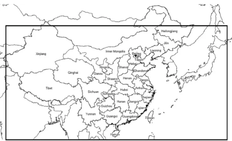
The modeling domain, shown in Fig. 3.1, with 36 × 36 km2 horizontal resolution

(163 × 97 horizontal grid cells), is centered over East Asia, including entire China, Northeast

Asian Countries such as Japan, North Korea and South Korea, parts of Southeast Asian

countries, such as Vietnam, and Thailand, and Northern part of India. The vertical structure