New developments in the ROOT fitting classes
XavierValls1,2,∗,LorenzoMoneta1,GuilhermeAmadio1, andArthurTsang3
1CERN, Geneva, Switzerland.
2Universitat Jaume I, Castelló de la Plana, C. Valenciana, Spain. 3Stanford University, Stanford, California, United States of America.
Abstract.
The ROOT Mathematical and Statistical libraries have been recently improved both to increase their performance and to facilitate the modelling of parametric functions that can be used for performing maximum likelihood fits to data sets to estimate parameters and their uncertainties.
First, we report on the new functionalities introduced in ROOT’s TFormula and TF1 classes to build these models in a convenient way for the users. We show how function objects, represented in ROOT by TF1 classes, can be used as probability density functions and how they can be combined together—via an addition operator—to perform extended likelihood fit of several normalized components. We also describe the new operators introduced to perform the convolution of two functions.
Finally, we report on the improvements in the performance of the ROOT fitting algorithm, by using SIMD vectorization when evaluating the model function on large data sets and by exploiting multi-thread parallelization when computing the likelihood function.
1 Introduction: Fitting and modeling in ROOT
Fitting of data distributions, a fundamental operation in High Energy Physics (HEP) analy-sis, is one of the most demanding and computing-intensive activities when performing data analysis on the results of the LHC.
ROOT [1] offers several techniques for fitting and modeling data distributions, from
in-tegration of the most popular minimizers, to objective function classes, to function classes for the user’s provided model function to interface with the minimizer. In this paper, we in-troduce the recent improvements implemented in the mathematical libraries that make fitting directly in ROOT easier and faster.
We extend the functionality of the TFormula class in ROOT, adding argument parsing and allowing to freely pass variables and parameters into pre-defined and user-defined func-tions. We also define a new syntax to use certain function compositions techniques, namely normalized sums and convolutions, directly in the TF1 function class. Finally, we introduce parallelization at data-level in the mathematical libraries and parallelization both at task-level and at data-level in the objective functions of the fitting, testing the potential to speed up parallelizable computations.
2 Modeling the fit with TFormula and TF1
ROOT’s fitting interfaces mainly rely on two classes to handle mathematical functions, TFor-mula and TF1. We introduce new developments in both classes, such as improved support and argument expression of TFormula function definitions and the introduction of new opera-tors in TF1 to express two methods of function composition: the normalized sum of functions and the convolution.
2.1 Extended support and improved argument expression in TFormula
TFormula provides the user with a convenient way to express mathematical functions as strings, e.g. "x+y[0]*59". These expressions are Just in time (JIT) compiled into C++
code.
Recently, we extended TFormula’s features with:
• Ordered and named parameters: we can specify which parameter to use from the parameter list by specifying its position. We can also name parameters to improve the readability of the formula (Listing 1, lines 1-4 ).
• Improved support for multi-dimensional functions: we added support to build TF2 and TF3 from TFormula expressions (Listing 1, lines 5-6 ).
• Concatenation of formula expressions: now it is possible to reuse previous declared func-tions in a new formula (Listing 1, lines 7-9 ).
1 // Ordered parameters
2 TF1 ("f1,"gaus( x,[0..2])+ gaus(x, [3],[4],[2])");
3 // Named parameters
4 TF1("f1","gaus(x, [Constant],[Mean],[Sigma])");
5 //Improved support for multi-dimensional functions
6 TF2 f2("f2","gaus( x+y, [A],[M],[S])");
7 //Concatenation of formula expressions
8 TF1 fs("sigma","[0]*x+[1]");
9 TF1 f1("f1","gaus(x,[C],[Mean],sigma(x,[A],[B])");
Listing 1: Examples of new ways of expressing parameters in TFormula.
2.2 New operators: Normalized Additions and Convolutions
Many typical HEP fits can be formulated as the sum of functions modeling different processes
as separate components (e.g. signal +background component). Fitting is often used to
determine the fractions or number of events involved in each one of these processes, in order to obtain relevant quantities and indicators, e.g. from the number of events we can obtain cross-sections and discovery significances.
When fitting for number of events, it is usually more interesting to normalize the diff
er-ent model functions before fitting instead of integrating them afterwards, which complicates the estimation of uncertainties due to correlations. Anormalized sumis a weighted sum of functions, fi, where the coefficients,ci, are computed after normalizing each function:
NS UM(f1, ...,f n)(x,p)=
n ∑
i=1
ci· fi(x,p)
fi(ξ,p)dξ, (1)
2 Modeling the fit with TFormula and TF1
ROOT’s fitting interfaces mainly rely on two classes to handle mathematical functions, TFor-mula and TF1. We introduce new developments in both classes, such as improved support and argument expression of TFormula function definitions and the introduction of new opera-tors in TF1 to express two methods of function composition: the normalized sum of functions and the convolution.
2.1 Extended support and improved argument expression in TFormula
TFormula provides the user with a convenient way to express mathematical functions as strings, e.g. "x+y[0]*59". These expressions are Just in time (JIT) compiled into C++
code.
Recently, we extended TFormula’s features with:
• Ordered and named parameters: we can specify which parameter to use from the parameter list by specifying its position. We can also name parameters to improve the readability of the formula (Listing 1, lines 1-4 ).
• Improved support for multi-dimensional functions: we added support to build TF2 and TF3 from TFormula expressions (Listing 1, lines 5-6 ).
• Concatenation of formula expressions: now it is possible to reuse previous declared func-tions in a new formula (Listing 1, lines 7-9 ).
1 // Ordered parameters
2 TF1 ("f1,"gaus( x,[0..2])+ gaus(x, [3],[4],[2])");
3 // Named parameters
4 TF1("f1","gaus(x, [Constant],[Mean],[Sigma])");
5 //Improved support for multi-dimensional functions
6 TF2 f2("f2","gaus( x+y, [A],[M],[S])");
7 //Concatenation of formula expressions
8 TF1 fs("sigma","[0]*x+[1]");
9 TF1 f1("f1","gaus(x,[C],[Mean],sigma(x,[A],[B])");
Listing 1: Examples of new ways of expressing parameters in TFormula.
2.2 New operators: Normalized Additions and Convolutions
Many typical HEP fits can be formulated as the sum of functions modeling different processes
as separate components (e.g. signal + background component). Fitting is often used to
determine the fractions or number of events involved in each one of these processes, in order to obtain relevant quantities and indicators, e.g. from the number of events we can obtain cross-sections and discovery significances.
When fitting for number of events, it is usually more interesting to normalize the diff
er-ent model functions before fitting instead of integrating them afterwards, which complicates the estimation of uncertainties due to correlations. Anormalized sumis a weighted sum of functions, fi, where the coefficients,ci, are computed after normalizing each function:
NS UM(f1, ...,f n)(x,p)=
n ∑
i=1
ci· fi(x,p)
fi(ξ,p)dξ, (1)
where NSUM is a numerical aproximation to the expression on the right.
If each figives a distribution of events from a given processi, then normalization has the
advantage thatcinow represents the count of these events.
TF1 is the ROOT class representing a one dimensional parametric function defined be-tween lower and upper limits. It can be constructed from a C++ free function pointer, a
TFormula-like expression or using a C++ function or callable object, e.g. a lambda or a
functor. In order to simplify performing normalized sum fits, we introduced in TF1 the new operator"NSUM", employed to create composite TF1 function objects from formula-based functions. Listing 2 showcases how to perform a fit with normalized sums.
// Model the background
TF1*expo2 = new TF1("expo2","[Constant]*exp([A0]*x + [A1]*x*x)",110,160); expo2->SetParameters(-8e-2, 2e-4, 5e5);
histo->Fit("expo2", "L");// binned Likelihood Fit // Modeling the full spectrum
TF1*model = new TF1("model","NSUM(expo2, gaus)", 110, 160); // new!
model->SetParameter(0, 1e4); // size of background
model->SetParLimits(1, 0, 1e3);// size of signal
model->SetParLimits(4, 115, 140);// mean
model->SetParLimits(5, .3, 6); // sigma
histo->Fit("model", "L");
Listing 2: Gaussian signal plus exponential background fit. We define first the background as a double exponential and then we model the full spectrum summing it with a Gaussian representing the signal.
The convolution of f andg, is defined as:
(f ∗g)(x)=
∫ inf
−inf f(ξ)g(x−ξ)dξ (2)
During HEP analysis, we often need to perform the convolution of two functions, e.g. when we compare against a model where f provides a theoretical distribution and ga res-olution function. We introduced the new "CONV" operator for building a TF1 function from the convolution of two functions. This operator is translated under the hood to the TF1Convolution class.
Listing 3 presents an example of the use of this operator to perform the convolution of a Breit-Wigner function and a Gaussian function. The convolution can be performed as an fast Fourier transform convolution (by default) or by applying numerical integration.
TF1*bw= new TF1("bw", "breitwigner", -15, 15); bw->SetParameters(1, 0, 1);
TF1 *mygausn = new TF1("mygausn", "gausn", -15, 15); mygausn->SetParameters(1, 0, 1);
TF1 *voigt = new TF1("voigt", "CONV(bw, mygausn)", -15, 15);
Listing 3: Code necessary for building a TF1 convolution of the Breit-Winger and Gaussian functions.
3 Multi-level parallelism in ROOT’s mathematical classes
In order to tackle the computational challenges posed by the ambitious physics program of the LHC, ROOT is undergoing a significant update, adapting its codebase for the efficient
exploitation of current and future hardware resources, where parallelism plays a central role. In the context of this extensive modernization effort, we provided data-level
3.1 Data-level parallelism
Data-level parallelism is achieved in ROOT by exploiting SIMD array operations (vector-ization). For this, we rely in the VecCore [2] vectorization library, which we integrated in ROOT’s mathematical libraries.
VecCore provides efficient vectorization by offering an extra layer of abstraction on top
of other vectorization libraries such as Vc and UME::SIMD. This extra layer of abstraction allows us to write portable, architecture-oblivious code, that will map to the system charac-teristics on compilation.
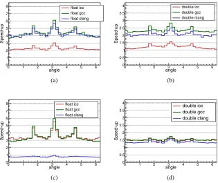
VecCore performance has been analyzed by computing, for different VecCore backends
and C++compilers, the Julia Setz2+0.7885eiα,α ∈ (0,2π] [3]. The results displayed in Figure 1 shows how Vc outperforms UME::SIMD every time and that gcc is the best compiler choice regarding performance when compiling with AVX2 as the instruction set.
0 1 2 3 4 5 6
angle
0 1 2 3 4 5 6 7 8
Speed-up
float icc float gcc float clang
(a)
0 1 2 3 4 5 6
angle
0 0.5 1 1.5 2 2.5 3 3.5 4
Speed-up
double icc double gcc double clang
(b)
0 1 2 3 4 5 6
angle
0 1 2 3 4 5 6 7 8
Speed-up
float icc float gcc float clang
(c)
0 1 2 3 4 5 6
angle
0 0.5 1 1.5 2 2.5 3 3.5 4
Speed-up
double icc double gcc double clang
(d)
Figure 1: Performance of the different compilers (clang 5, gcc 7 and icc 17), when evaluating
the Julia Setz2+0.7885eiαwith the angleα ∈ (0,2π] on arrays of float and double SIMD types for VecCore’s Vc (1a and 1b) and UME::SIMD (1c and 1d) backends.
3.1 Data-level parallelism
Data-level parallelism is achieved in ROOT by exploiting SIMD array operations (vector-ization). For this, we rely in the VecCore [2] vectorization library, which we integrated in ROOT’s mathematical libraries.
VecCore provides efficient vectorization by offering an extra layer of abstraction on top
of other vectorization libraries such as Vc and UME::SIMD. This extra layer of abstraction allows us to write portable, architecture-oblivious code, that will map to the system charac-teristics on compilation.
VecCore performance has been analyzed by computing, for different VecCore backends
and C++compilers, the Julia Setz2 +0.7885eiα,α ∈ (0,2π] [3]. The results displayed in Figure 1 shows how Vc outperforms UME::SIMD every time and that gcc is the best compiler choice regarding performance when compiling with AVX2 as the instruction set.
0 1 2 3 4 5 6
angle 0 1 2 3 4 5 6 7 8 Speed-up float icc float gcc float clang (a)
0 1 2 3 4 5 6
angle 0 0.5 1 1.5 2 2.5 3 3.5 4 Speed-up double icc double gcc double clang (b)
0 1 2 3 4 5 6
angle 0 1 2 3 4 5 6 7 8 Speed-up float icc float gcc float clang (c)
0 1 2 3 4 5 6
angle 0 0.5 1 1.5 2 2.5 3 3.5 4 Speed-up double icc double gcc double clang (d)
Figure 1: Performance of the different compilers (clang 5, gcc 7 and icc 17), when evaluating
the Julia Setz2+0.7885eiαwith the angleα∈ (0,2π] on arrays of float and double SIMD types for VecCore’s Vc (1a and 1b) and UME::SIMD (1c and 1d) backends.
We applied vectorization in several places in ROOT, fundamentally in the mathe-matical functions. For user convenience, we introduced two new ROOT SIMD types, ROOT::Double_v and ROOT::Float_v. TF1 now accepts user functions built with ROOT::Double_vdata and return types, and TFormula data types can be compiled to ROOT SIMD types by callingTFormula::SetVectorized()orTF1::SetVectorized().
Figure 2 compares, for the evaluation of two different operations, the difference in
per-formance of a free C++function vectorized, a TF1 built from a vectorized free function and
a TF1 built from a formula and then set to vectorized.
CASE 1 CASE 2
0 0.5 1 1.5 2 2.5 3 3.5 4
Speed-up
Vectorization Performance on AVX2
C++ Function TF1 Compiled TF1 Formula
Figure 2: Performance of the vectorization of a free function, a TF1 and a TF1 built from a formula for the evaluation of two different operations, the evaluation of a 2nd degree
polyno-mial (CASE1) and the sum of and exponential and a Gaussian function (CASE 2).
3.2 Task-level parallelism
We exploit task-level parallelism in ROOT with the executors [4], which are highly-reusable implementations of the Map-Reduce pattern recently introduced in ROOT that offer a flexible
and convenient programming model and remarkable performance.
ROOT offers several executors that have been deployed successfully throughout ROOTs
codebase:
• TSequentialExecutor, a sequential implementation of the MapReduce pattern. • TProcessExecutor, a fork-based multiprocess executor.
• TThreadExecutor, a TBB-based multithreaded one.
• TNUMAExecutor, a proof of concept aiming at reducing the negative impact of remote memory accesses in NUMA systems by integrating TProcessExecutor, TThreadExecutor and libnuma [3].
3.3 The fitting case
VecCore and the executors are applied together in order to achieve the multi-level paralleliza-tion of the fitting process [5].
the formula expression to be compiled withROOT::Double_vdata types instead ofdouble
types.
1 // Enable implicit parallelization
2 ROOT::EnableImplicitMT();
3 std::string func = " [0] * exp(-(*data + (-130.)) * (*data + (-130.)) / 2) + \
4 [1] * exp(-([2] * (*data * (0.01)) - [3] * ((*data) * (0.01)) * ((*data) * (0.01))))";
5 autof = TF1("fParallel", func.c_str(), 100, 200, 4);
6 f.SetParameters(1, 1000, 7.5, 1.5);
7 // Enable the vectorized evaluation of the function
8 f.SetVectorized()
9 TH1D h1f("h1f", "Test random numbers", 12800, 100, 200);
10 h1f.FillRandom("fvCore", 1000000);
11 h1f.Fit(&f);
Listing 4: Vectorized and parallelized fit, built from a ROOT formula, of the invariant mass distribution for the diphoton system resulting from the decay of a Higgs boson.
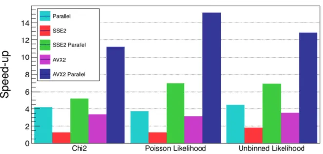
Figure 3: Performance of the multithreaded and vectorized parallelization of the fit with different objective functions and different set of instructions (SSE, or Streaming SIMD Ex-tensions, and AVX2 or Advanced Vector Extensions 2, in an Intel Core i7-4790 processor with 4 physical cores and 8GB of RAM.
Figure 3 presents the performance of evaluating each type of parallelized objective func-tion when fitting for the invariant mass spectrum to determine significance and locafunc-tion of the signal (e.g. H− > γγ). The results obtained are good when vectorizing and excellent when parallelizing on several cores, obtaining the most outstanding results when applying simultaneously data-level and task-level parallelization.
4 Conclusions
In the context of ROOT’s modernization effort, the mathematical and statistical libraries are being improved, extending their functionalities and features and adapting their code for par-allelism, capitalizing on the performance the current architectures have to offer.
the formula expression to be compiled withROOT::Double_vdata types instead ofdouble
types.
1 // Enable implicit parallelization
2 ROOT::EnableImplicitMT();
3 std::string func= " [0] * exp(-(*data + (-130.)) * (*data + (-130.)) / 2) + \
4 [1] * exp(-([2] * (*data * (0.01)) - [3] * ((*data) * (0.01)) * ((*data) * (0.01))))";
5 auto f = TF1("fParallel", func.c_str(), 100, 200, 4);
6 f.SetParameters(1, 1000, 7.5, 1.5);
7 // Enable the vectorized evaluation of the function
8 f.SetVectorized()
9 TH1D h1f("h1f", "Test random numbers", 12800, 100, 200);
10 h1f.FillRandom("fvCore", 1000000);
11 h1f.Fit(&f);
Listing 4: Vectorized and parallelized fit, built from a ROOT formula, of the invariant mass distribution for the diphoton system resulting from the decay of a Higgs boson.
Figure 3: Performance of the multithreaded and vectorized parallelization of the fit with different objective functions and different set of instructions (SSE, or Streaming SIMD Ex-tensions, and AVX2 or Advanced Vector Extensions 2, in an Intel Core i7-4790 processor with 4 physical cores and 8GB of RAM.
Figure 3 presents the performance of evaluating each type of parallelized objective func-tion when fitting for the invariant mass spectrum to determine significance and locafunc-tion of the signal (e.g. H− > γγ). The results obtained are good when vectorizing and excellent when parallelizing on several cores, obtaining the most outstanding results when applying simultaneously data-level and task-level parallelization.
4 Conclusions
In the context of ROOT’s modernization effort, the mathematical and statistical libraries are being improved, extending their functionalities and features and adapting their code for par-allelism, capitalizing on the performance the current architectures have to offer.
TFormula and TF1 are at the core of ROOT’s mathematical functionalities. We enhanced TFormula’s parameter expression, allowing position-aware and named parameters. In addi-tion, we added support for TFormula constructors in multidimensional function classes (TF2,
TF3). TF1’s formula constructor has been extended with the addition of two new operators to generate composite functions,NSUMandCONV, implementing, respectively, the normalized sum and the convolution of two functions.
We introduced a new library in ROOT, VecCore, to implement data-level parallelism in ROOT. VecCore allows for the right level of abstraction from compiler intrinsics and pro-vides a convenient programming model for the user. We analyzed VecCore’s performance with different combinations of data types, backends and compilers, concluding that gcc 7 outperforms clang 5 and icc 17, and suggesting to choose Vc over UME::SIMD.
Finally, we demonstrated that the fitting is a perfect candidate for applying paralleliza-tion at multiple levels, by exploiting VecCore and the new parallel MapReduce classes—the executors, obtaining remarkable speed-ups when vectorizing and close to ideal when paral-lelizing the fit over multiple cores, resulting in an increase in performance severalfold without impacting the programming model.
References
[1] R. Brun, F. Rademakers,ROOT - An Object Oriented Data Analysis Framework, in
Pro-ceedings AIHENP’96 Workshop, edited by N. Inst., M. in Phys. (1997), Vol. A389, pp.
81–86,http://root.cern
[2] G. Amadio, P. Canal, S. Wenzel, root-project/veccore: Release v0.4.2 (2017),https: //github.com/root-project/veccore/
[3] X. Valls Pla, Ph.D. thesis, Universitat Jaume I (2018)
[4] P. Canal, G. Ganis, E. Guiraud, P. Mato Vila, L. Moneta, D. Piparo, E. Tejedor, X. Valls
Pla,Expressing Parallelism in ROOT, in22nd International Conference on Computing
in High Energy and Nuclear Physics(IOP, in press)