Bayesian Estimation of the Survival Function

(1)

ISSN(Online): 2319-8753 ISSN (Print): 2347-6710

I

nternational

J

ournal of

I

nnovative

R

esearch in

S

cience,

E

ngineering and

T

echnology

(A High Impact Factor & UGC Approved Journal) Website: www.ijirset.com

Vol. 6, Issue 9, September 2017

Bayesian Estimation of the Survival Function

A. Lavanya

1

,

T. Leo Alexander

2

Research Scholar, Department of Statistics, Loyola College, Chennai–34, India1

Associate Professor, Department of Statistics, Loyola College, Chennai–34, India2

ABSTRACT: Weibull distribution is one of the most important lifetime distributions that is used for modeling and analysing data in clinical, life sciences and engineering. The main objective of this paper was to determine the best Bayesian Survival estimator for the Constant Shape Bi-Weibull distribution. The methods under consideration are the Bayesian estimator by using three loss functions, which are Linear Exponential (LINEX) loss, General Entropy loss and Squared Error loss function. Lindley approximation is used to obtain the Bayes estimators. Comparisons are made through simulation study to determine the performance of these methods. An illustrative example is also provided to explain the concepts.

KEYWORDS: Bayesian, MLE, Jeffreys Prior information, Extension of Jeffreys Prior information, Lindley approximation.

I. INTRODUCTION

Weibull distribution is mostly used for failure time in both lifetime and reliability analysis. It was mostly very useful for modeling and analyzing life time data in the applied and engineering sciences [1]. In [2] stated that the advantage of Weibull analysis is its ability to provide accurate failure analysis and failure forecasts with extremely smaller samples. Previously Bayesian survival estimator for Weibull distribution with censored data was discussed in [3]. In this paper the main consideration is to determine the best Bayesian Survival estimator for the Constant Shape Bi-Weibull distribution by using three loss functions, which are Linear Exponential (LINEX) loss, General Entropy loss and Squared Error loss function. Lindley approximation is used to obtain the Bayes estimators.

We also studied Estimation of the Survival Function under the Constant Shape Bi-Weibull Failure Time Distribution Based on Three Loss Functions [4], we used only Extension of Jeffreys prior information but in this paper we have to use both methods, namely, Extension of Jeffreys prior information and Jeffrey’s prior information for best Bayesian Survival Estimator.

This paper is organized as follows. In the Section 2, Bayesian estimation of Survival function under Jeffreys’ Prior Information and Extension of Jeffreys’ Prior Information with Three Loss functions is discussed. Section 3, provides simulation study carried out to investigate the performance of the Survival estimators. In Section 4, the proposed theory is validated by using simulated data. This is followed by results and finally conclusion is given in section 5.

II. BAYESIAN ESTIMATION OF SURVIVAL FUNCTION

Let t1, t2 … tn be a random sample of size n with respect to the Constant Shape Bi-Weibull distribution, with σ and β as the parameters, where σ is the scale parameter and β is the shape parameter. The probability density function ( ), cumulative distribution function ( ) and survival function are given, respectively, as follows:

( ; , ) = . (1) The Cumulative distribution function (CDF) is

( ; , ) = 1− . (2)

The Survival function is

(2)

I

nternational

J

ournal of

I

nnovative

R

esearch in

S

cience,

E

ngineering and

T

echnology

For analysing Failure time data Bayesian survival estimation approach has received a lot of attention. Prior Distribution and the Loss Function in Bayesian analysis the choice of prior is inevitable. The choice of a prior, most often does not depend on ones subjective knowledge and beliefs.

The likelihood function of the selected sample is given by

( , , ) = . (4) The log-likelihood function is

= + ( −1) − −1 . (5)

The Bayes estimators of the parameters are considered with different loss functions which are given below:

Linexloss:L θ−θ ∝exp a θ−θ −a θ−θ −1 (6)

Generalentropyloss:L θ−θ ∝ θ − θ −1 (7)

and SquaredErrorloss:L θ−θ ∝ θ−θ . (8)

A. JEFFREY’S PRIOR INFORMATION:

Consider a likelihood function L(θ), with its Fisher Information ( ) = −E

β . The Fisher Information measures

the sensitivity of an estimator. Jeffreys suggested that ( )∝[ ( )] be considered as a prior for the likelihood

function L(θ).

The Jeffreys prior is justified on the grounds of its invariance under parameterization according to Sinha [5]. Under the two-parameter Weibull distribution the non-informative (vague) prior according to Sinha and Sloan [6] is given as

( , )∝ 1 .

Let the likelihood equation which is ( | , )being the same as (6). The joint posterior of the parameters σ and β is given by

π(σ,β|t)∝L(t|σ,β)v(σ,β). (9) The marginal distribution function is the double integral of equation (9). Therefore, the posterior probability density function of σ and β given the data (t1, t2, …, tn) is obtained by dividing the joint posterior density function over the marginal distribution function as

π∗(σ,β|t) = L(t|σ,β)v(σ,β)

∬L(t|σ,β)v(σ,β) . (10)

B. EXTENSION OF JEFFREY’S PRIOR INFORMATION

We propose a Extension of Jeffreys Prior information such that,

( )∝ 1 .

(3)

I

nternational

J

ournal of

I

nnovative

R

esearch in

S

cience,

E

ngineering and

T

echnology

information approach is employed on both parameters. It is important that one ensures the prior does not significantly influence the final result. If our limited or lack of knowledge influences the results, then one may end-up giving wrong interpretations, which could affect whatever we seek to address. It is as a result of this that the Extension of Jeffreys Prior information is considered.

We have,

( , )∝ 1 .

The likelihood function from equation (4) is

( | , ) = .

According to Bayes theorem, the joint posterior distribution of the parameters σ and β is

π∗(σ,β|t)∝L(t|σ,β)u(σ,β), where

( | , ) =

( )

and the marginal distribution is

( ) ,

where k is the normalizing constant that makes π∗ a proper pdf. The posterior density function is obtained by using equation (10).

In recent times for analyzing Failure Time data Bayesian Estimation approach has received a lot of attention, which has mostly used to compare the traditional methods.

It may be note that by taking into account our prior information which is essential, the Bayes estimator shall be considered with respect to three loss functions which are also indisputable in Bayesian estimation.

REMARK:

Here we consider two Asymmetric Loss Functions namely Linear Exponential (LINEX) Loss Function and General Entropy Loss Function. Also the Symmetric Loss Function namely Squared Error Loss Function considered in order to estimate Survival Function.

C. LINEAR EXPONENTIAL LOSS FUNCTION (LINEX):

The LINEX Loss Function is under the assumption that the minimal loss occurs at θ=θand is expressed as L θ−θ ∝exp a θ−θ −a θ−θ −1,

where is an estimation of θ and a≠0. The sign and magnitude of the shape parameter ‘a’ represents the direction and degree of symmetry, respectively. There is overestimation if a > 0and underestimation if a < 0but when ≅0 , the LINEX Loss Function is approximately the Squared Error Loss Function. The posterior expectation of the LINEX Loss Function, according to [10], is

− ∝ (exp(− ))− − ( ) −1. (11) The Bayes Estimator of θ, represented by under LINEX Loss Function, is the value of which minimizes equation (11) and is given as

=−1 ( (− )).

Provided ( (− ) exists and is finite.

(4)

I

nternational

J

ournal of

I

nnovative

R

esearch in

S

cience,

E

ngineering and

T

echnology

( ) = − | =

∬ − ∗_{( , )}

∬ ∗_{( , )} . (12)

From (12), it can be observed that ratio of integrals which cannot be solved analytically and so we employ Lindley’s approximation procedure to estimate the parameters. Lindley considered an approximation for the ratio of integrals for evaluating the posterior expectation of an arbitrary function ( ) as

[ ( )| ] =∫ ( ) ( )[ ( )]

∫ ( )[ ( )] . According to [6], Lindley’s expansion can be approximated asymptotically by

= +1

2[ + ] + + +

1

2 + , (13) where L is the log-likelihood function in equation (5),

= − ,

= ,

= = , = = + ,

= = , = = ( ) + ,

= (− ) , = (− ) .

=− −1 ( ) ,

= 2 − ∑ ( ) ,

= −2∑ , =−2 + 6∑ .

For Extension of Jeffreys Prior information

( , ) =− ( )− ( ), = =− = =− .

For Jeffreys Prior information

( , ) =− ( )− ( ), = =− = =− .

Bayesian Estimation of Survival Function using LINEX Loss Function is given as ( ; , ) = .

D. GENERAL ENTROPY LOSS FUNCTION:

Another useful Asymmetric Loss Function is the General Entropy (GE) Loss which is a generalization of the Entropy

Loss and is given as L θ−θ ∝ θ − θ −1 .

The Bayes Estimator of θunder the General Entropy Loss is =[ ( )] , provided ( )exists and is finite. The posterior density function of the Survival function under general entropy loss is given as

( ) = − | =

∬ − ∗_{( , )}

(5)

I

nternational

J

ournal of

I

nnovative

R

esearch in

S

cience,

E

ngineering and

T

echnology

Applying the same Lindley approach here as in (13) with u1, u11 and u2, u22 are the first and second derivatives for σ and β, respectively, and are given as

= , = ,

= = , = = − ,

=− ( ) = =− ( ) + ( ) .

Bayesian Estimation of Survival Function using General Entropy Loss Function is given as ( ; , ) = .

E. SYMMETRIC LOSS FUNCTION:

The Symmetric Loss Function is the Squared Error Loss is given by L θ−θ ∝ θ−θ .

This Loss Function is symmetric in nature, that is, it gives equal weightage to both over and under estimation. In real life, we encounter many situations where overestimation may be more serious than underestimation or vice versa. The most common loss function used for Bayesian estimation is the squared error (SE), also called quadratic loss. The square error loss denotes the punishment in using to θestimate θ and is given as ( | ) = θ(t)−θ , where the expectation is taken over the joint distribution of θ and (t).

The posterior density function of the Survival function under the Symmetric loss function are given as

( ) = − | =

∬ − ∗_{( , )}

∬ ∗_{( , )} .

Applying the same Lindley approach here as in (13) with u1, u11 and u2, u22 are the first and second derivatives for σ and β, respectively, and are given as

= , = ,

= = , = = − ,

= ( ) = = ( + 1).

Bayesian Estimation of Survival Function using Symmetric Loss Function is given as ( ; , ) = .

III.SIMULATION STUDY

Since it is difficult to compare the performance of the estimators theoretically and also to validate the data employed in this paper, we have performed extensive simulations to compare the estimators through Mean Squared Errors and Absolute Biases by employing different sample sizes with different parameter values. The Mean Squared Error and

Absolute Bias given as =∑ =∑ .

In our Simulation study, we chose a sample size of n= 25, 50, and 100 to represent small, medium, and large dataset. The Survival function is estimated for Constant Shape Bi-Weibull distribution with Bayesian using Extension of Jeffreys’ Prior method and Jeffreys’ Prior method.

The values of the parameters chosen are = 0.5and1.5, = 0.8and1.2. The values of Jeffreys Extension are = 0.4and 1.4. The Loss parameters values are = = (±0.6, ±1.6). These were iterated (R) 5000 times and the Survival function for each method was calculated. The results are presented below for the estimated Survival function and their corresponding Mean Squared Error and Absolute Bias values.

(6)

I

nternational

J

ournal of

I

nnovative

R

esearch in

S

cience,

E

ngineering and

T

echnology

Table 1: MSE Estimated Survival function using extension of Jeffrey’s prior information

From Table 1 it is observed that Bayes estimation with LINEX loss function provides the smallest MSE values in most cases especially the loss parameter value is 0.6. Also when sample size increases Bayes estimation under all loss functions have increases in MSE values.

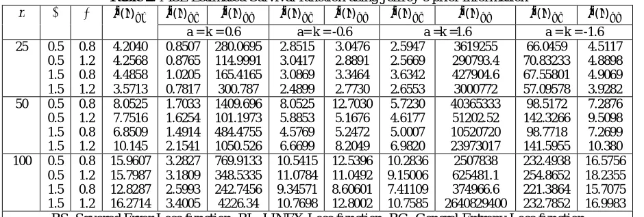
In Table 2 we present the Mean Square Error estimated values for the Survival function S(t) for Bayesian Estimation using Jeffrey’s prior information with the three loss functions.

Table 2: MSE Estimated Survival function using Jeffrey’s prior information

From Table 2 it is observed that Bayes estimation with LINEX loss function provides the smallest MSE values in most cases especially the loss parameter value is 0.6. Also when sample size increases Bayes estimation under all loss functions have increases in MSE values.

n σ c β ( ) ( ) ( ) ( ) ( ) ( ) ( ) ( ) ( )

a = k = 0.6 a= k = -0.6 a =k =1.6 a = k = -1.6

25 0.5 0.5 0.5 0.5 1.5 1.5 1.5 1.5 0.4 1.4 0.4 1.4 0.4 1.4 0.4 1.4 0.8 0.8 1.2 1.2 0.8 0.8 1.2 1.2 4.2007 4.2695 4.2584 4.4609 4.4838 4.5255 3.5733 3.5633 0.8488 0.8889 0.8739 0.3570 1.0216 1.0786 0.7831 0.8028 283.32 222.49 116.83 6.4981 163.43 175.05 298.91 162.10 2.8479 2.9214 3.0369 1.8970 3.0882 3.4672 2.4931 2.1534 3.0503 3.0062 2.8955 1.6525 3.3407 3.2399 2.7722 2.9026 2.5868 2.7562 2.5562 0.7064 3.6395 3.7418 2.6609 2.8644 3706865 2108747 301937.8 162.5991 418602 869294.6 2972000 305725.5 66.008 66.675 70.796 59.478 67.561 79.953 57.149 39.212 4.5070 4.6025 4.8910 4.6074 4.9069 5.3834 3.9302 3.2469 50 0.5 0.5 0.5 0.5 1.5 1.5 1.5 1.5 0.4 1.4 0.4 1.4 0.4 1.4 0.4 1.4 0.8 0.8 1.2 1.2 0.8 0.8 1.2 1.2 8.0489 7.6888 7.7564 6.4410 6.8489 7.1812 10.146 7.6612 1.7025 1.5836 1.6212 1.4276 1.4921 1.5218 2.1550 1.6268 1415.261 1066.58 102.2422 56.94168 480.746 132.2614 1047.962 893.232 4.9239 5.1215 5.8756 4.9212 4.5774 4.9586 6.6714 5.1654 6.9123 6.0518 5.1781 4.0470 5.2423 4.9977 8.2033 5.8401 5.7190 4.9388 4.6015 4.1203 5.0041 4.6629 6.9864 5.1644 40735862 5025113880 52547.17 20207.87 10373194 213972.6 23857352 58425573 98.5131 113.234 142.192 111.920 98.7605 107.548 141.605 112.276 7.2818 8.0862 9.5131 7.7936 7.2698 8.0903 10.383 8.2034 100 0.5 0.5 0.5 0.5 1.5 1.5 1.5 1.5 0.4 1.4 0.4 1.4 0.4 1.4 0.4 1.4 0.8 0.8 1.2 1.2 0.8 0.8 1.2 1.2 15.9599 16.2185 15.8053 16.1742 12.8229 17.9673 16.2717 17.8387 3.2816 3.3791 3.1785 3.3046 2.6007 3.6025 3.4014 3.7973 771.6215 991.9134 350.2333 553.6934 241.7176 573.0519 4220.786 5046.634 10.539 10.476 11.074 11.677 9.3481 13.268 10.771 11.461 12.5423 12.9333 11.0590 11.4502 8.59889 12.1827 12.7988 15.1484 10.2787 10.7703 9.1398 9.5553 7.41679 10.1714 10.7625 12.4771 2522011 5437513 633570.3 1869227 371204.2 5510193 2634290550 833552987 232.4689 221.4281 254.8635 275.4141 221.3958 324.8459 232.7989 237.7222 16.5723 16.2057 18.2381 19.0687 15.7038 22.2644 17.0002 17.4871 BS: Squared Error Loss function, BL: LINEX Loss function, BG: General Entropy Loss function

n Σ β ( ) ( ) ( ) ( ) ( ) ( ) ( ) ( ) ( )

a = k = 0.6 a= k = -0.6 a =k =1.6 a = k = -1.6 25 0.5

0.5 1.5 1.5 0.8 1.2 0.8 1.2 4.2040 4.2568 4.4858 3.5713 0.8507 0.8765 1.0205 0.7817 280.0695 114.9991 165.4165 300.787 2.8515 3.0417 3.0869 2.4899 3.0476 2.8891 3.3464 2.7730 2.5947 2.5669 3.6342 2.6553 3619255 290793.4 427904.6 3000772 66.0459 70.83233 67.55801 57.09578 4.5117 4.8898 4.9069 3.9282 50 0.5

0.5 1.5 1.5 0.8 1.2 0.8 1.2 8.0525 7.7516 6.8509 10.145 1.7033 1.6254 1.4914 2.1541 1409.696 101.1973 484.4755 1050.526 8.0525 5.8853 4.5769 6.6699 12.7030 5.1676 5.2472 8.2049 5.7230 4.6177 5.0007 6.9820 40365333 51202.52 10520720 23973017 98.5172 142.3266 98.7718 141.5955 7.2876 9.5098 7.2699 10.380 100 0.5

(7)

I

nternational

J

ournal of

I

nnovative

R

esearch in

S

cience,

E

ngineering and

T

echnology

In Table 3 we present the Absolute Bias estimated values for the Survival function S(t) for the Bayesian Estimation using extension of Jeffrey’s prior information with the three loss functions.

Table 3: Absolute Bias Estimated Survival function using extension of Jeffrey’s prior information

From Table 3 it is observed that Bayes estimation with LINEX loss function provides the smallest Absolute Bias values in most cases. As the sample size increases Absolute values of the Bayes estimation under all loss functions increases. In Table 4 we present the Absolute Bias estimated values for the Survival function S(t) for the Bayesian Estimation using Jeffrey’s prior information with the three loss functions.

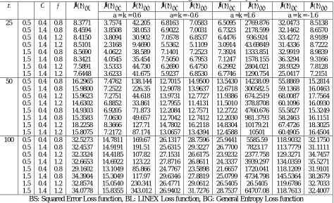
Table 4: Absolute Bias Estimated Survival function using Jeffrey’s prior information

n σ C β ( ) ( ) ( ) ( ) ( ) ( ) ( ) ( ) ( )

a = k = 0.6 a= k = -0.6 a =k =1.6 a = k = -1.6 25 0.5

0.5 0.5 0.5 1.5 1.5 1.5 1.5 0.4 1.4 0.4 1.4 0.4 1.4 0.4 1.4 0.8 0.8 1.2 1.2 0.8 0.8 1.2 1.2 8.3771 8.4594 8.4150 8.5101 8.5690 8.3421 7.5891 7.6448 3.7574 3.8508 3.8094 2.3168 4.0622 4.0545 3.5333 3.6233 42.205 38.053 30.902 9.4690 38.589 35.454 44.730 41.675 6.8163 6.9022 7.0578 5.5362 7.1401 7.5050 6.2690 5.9237 7.0583 7.0031 6.8537 5.1109 7.2523 6.7953 6.4750 6.8530 6.5095 6.7323 6.4476 3.0914 7.3924 7.1247 6.2992 6.7746 2769.876 2178.599 936.924 43.69849 1333.851 1578.155 2804.021 1290.754 32.0473 32.1462 33.4272 31.4336 32.9919 36.3294 28.9329 25.0417 8.5138 8.6570 8.9189 8.7222 8.9839 9.3166 7.8128 7.2151 50 0.5

0.5 0.5 0.5 1.5 1.5 1.5 1.5 0.4 1.4 0.4 1.4 0.4 1.4 0.4 1.4 0.8 0.8 1.2 1.2 0.8 0.8 1.2 1.2 16.2965 15.9800 15.9623 14.6302 14.9303 15.3583 18.2258 15.8075 7.4762 7.2522 7.2751 6.8852 6.9205 7.0630 8.3666 7.2172 138.144 226.35 44.618 33.861 71.873 49.657 127.71 87.174 12.7015 12.9078 13.9731 12.7955 12.2084 12.7042 14.7802 13.0657 14.9500 13.9637 12.7727 11.4131 12.7571 12.7412 16.2118 13.4394 13.5430 12.6718 11.9386 11.5010 12.2722 12.2030 14.8304 12.4588 14238.09 300582.5 674.2519 378.8708 4760.676 981.3793 10179.21 10501 55.8869 59.1368 68.0087 60.1096 55.5827 58.2463 67.4726 60.4905 15.2814 16.0463 17.7564 16.0930 15.3249 16.1151 18.3025 16.4504 100 0.5

0.5 0.5 0.5 1.5 1.5 1.5 1.5 0.4 1.4 0.4 1.4 0.4 1.4 0.4 1.4 0.8 0.8 1.2 1.2 0.8 0.8 1.2 1.2 32.5273 32.4537 32.3324 32.6653 29.1602 34.3904 32.8574 34.0778 14.7811 14.9191 14.4185 14.6922 13.1049 15.3049 15.0540 15.8355 169.67 191.51 107.82 123.22 85.866 117.97 230.341 343.012 26.1317 25.6315 27.1531 27.8716 24.7767 29.6346 26.4771 26.9402 28.7596 29.3227 26.6175 26.8611 23.5898 27.8819 29.0612 31.7276 25.9441 26.7700 23.9232 24.3337 21.6657 25.0799 26.5405 28.7537 5585.59 7823.17 2377.758 3939.297 1720.041 4734.798 26.5405 64707.08 118.9032 113.7779 129.3271 134.0359 118.1209 145.5364 119.6786 118.7613 32.1750 31.1111 34.7457 35.5271 31.9101 38.2679 32.7033 32.4007 BS: Squared Error Loss function, BL: LINEX Loss function, BG: General Entropy Loss function

n Σ β ( ) ( ) ( ) ( ) ( ) ( ) ( ) ( ) ( )

a = k = 0.6 a= k = -0.6 a =k =1.6 a = k = -1.6 25 0.5

0.5 1.5 1.5 0.8 1.2 0.8 1.2 8.3815 8.4140 8.5709 7.5852 3.7619 3.8157 4.0598 3.5293 41.999 30.700 38.792 44.849 6.8206 7.0640 7.1383 6.2641 7.0550 6.8463 7.2585 6.4754 6.5201 6.4624 7.3862 6.2904 2742.315 922.4347 1346.016 2815.518 32.0535 33.43658 32.9926 28.9180 8.5206 8.9204 8.9829 7.8079 50 0.5

0.5 1.5 1.5 0.8 1.2 0.8 1.2 16.3005 15.9568 14.9320 18.2252 7.4783 7.2864 6.9184 8.3646 137.897 44.4053 72.0825 127.8573 12.7030 13.9866 12.2072 14.7785 14.9492 12.7591 12.7631 16.2135 13.5484 11.9630 12.2666 14.8252 14182.55 666.7129 4788.059 10199.89 55.8865 68.0421 55.5876 67.4715 15.2890 17.7560 15.3236 18.2997 100 0.5

(8)

I

nternational

J

ournal of

I

nnovative

R

esearch in

S

cience,

E

ngineering and

T

echnology

From Table 4 it is observed that Bayes estimation with LINEX loss function provides the smallest Absolute Bias values in most cases. As the sample size increases Absolute values of the Bayes estimation under all loss functions increases.

IV.ILLUSTRATION

The real data set is about a clinical Trial in the Treatment of Carcinoma of the Oropharynx (PHARYNX) Data extracted from [7]. The data file gives the data for a part of a large clinical trial carried out by the Radiation Therapy Oncology Group in the United States. This data consists of a total of 195 respondents of which 53 are alive and 142 are dead. Here we considered Survival time in days from day of diagnosis is the most factor.

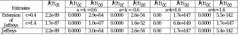
Table 5 depicts the Standard Error values for Estimated Survival function S(t) using PHARYNX Data. So the Survival function is estimated for Constant Shape Bi-Weibull distribution with Bayesian using Extension of Jeffreys’ Prior method and Jeffreys’ Prior method.

Table 5: Standard Error values for Estimated Survival function S(t) using PHARYNX Data

Estimates

( ) ( ) ( ) ( ) ( ) ( ) ( ) ( ) ( )

a = k = 0.6 a= k = -0.6 a=k=1.6 a=k=-1.6 Extension

of Jeffreys

c=0.4 2.2e-89 0.0000 2.9e+54 0.0000 2.6e-54 0.00 1.7e+147 0.0000 5.5e-142

c=1.4 1.7e-87 0.0000 1.0e+57 0.0000 1.6e-52 0.00 6.8e+149 0.0000 1.7e+147

Jeffreys 2.2e-89 0.0000 3.0e+54 0.0000 2.6e-54 0.00 1.7e+147 0.0000 5.4e-142

From Table 5, we observe that, Bayesian estimator under LINEX loss function has the smallest values for Survival function S(t). So that the Bayes estimators of Survival function S(t) using Extension of Jeffreys’ Prior method and Jeffreys’ Prior method under LINEX loss function is best estimation method for Constant Shape Bi-Weibull Distribution using PHARYNX Data.

V. CONCLUSION

In this paper, we observed that the problem of Bayesian estimation of Survival function for the Constant Shape Bi-Weibull distribution, under Asymmetric and Symmetric loss functions. Bayes estimators were obtained using Lindley approximation method. A Simulation study was conducted to examine and compare the performance of the estimators for different sample sizes with different values for the extension of Jeffreys’ prior and the loss functions. From the results, we observe that in most cases, Bayesian estimator under LINEX loss function has the smallest Mean Squared Error values and minimum Bias for Survival function S(t) in most cases especially compared to the loss parameter values are 0.6 and 1.6, for both values of the extension of Jeffreys’ prior information. As the sample size increases the Mean Squared Error and the Absolute Bias for Bayes estimator under all the loss functions increases correspondingly.

REFERENCES

[1] Lawless, J. F., “Statistical Models and Methods for Lifetime Data”, John Wiley & Sons, New York, NY, USA, 1982. [2] Abernethy, R.B., “The New Weibull Handbook”, 5th edition, 2006.

[3] Al Omari, M.A., and Ibrahim, N.A., “Bayesian survival estimation for Weibull distribution with censored data”, Journal of Applied Sciences, 11(2), 393–396, 2011.

[4] Lavanya, A., and Leo Alexander, T., “Estimation of The Survival Function under The Constant Shape Bi-Weibull Failure Time Distribution Based on Three Loss Functions”, International Journal of advanced Research, 4(9), 1225-1234, 2016.

[5] Sinha, S. k., and Sloan, J. A., “Bayes Estimation of the Parameters and Reliability Function of the 3-Parameter Weibull Distribution”, IEEE Transactions on Reliability, 37, 364-369, 1988.

[6] Sinha, S. K., “Bayes Estimation of the Reliability Function and Hazard Rate of a Weibull Failure Time Distribution”, Tranbajos De Estadistica, 1, 47-56, 1986.