Performance Model for a Public Logistics Network

ABSTRACT

XIANG, LING. Performance Model for a Public Logistics Network. (Under the direction of

Michael G. Kay.)

A public logistics network (PLN) has been proposed as an alternative to private networks for

the ground transport of parcels. In this dissertation, a heuristic approach to approximate the

package average waiting time in a PLN is presented; and then based on this waiting time

approximation, a PLN design procedure is developed.

A PLN can be viewed as a priority queuing network with bulk arrivals and bulk service. It is

difficult to obtain a closed-form solution for package average waiting time in a PLN. The

problem is reformulated so that trucks transport loads instead of individual packages, thereby

relaxing the bulk arrivals and bulk service feature. The package average waiting time is

approximated fairly accurately by Kingman’s equation when the server utilization is high.

A simulation model is created to determine the parameters needed in Kingman’s equation

(the coefficient of variation for package interarrival times and for truck interarrival times). A

regression analysis of the results shows that the headway ratio is around 5.5. The package

average waiting time is approximated by the product of the truck headway (truck average

The PLN simulation with protocols and the package bidding process is discussed as an

extension to the basic simulation model. Packages bid for their trips along the way. The

highest bidder gets the highest priority for truck transport services. Results from a simulation

model incorporating a series of protocols developed by Kay show that a PLN with these

protocols performs better than a FIFO system.

For the PLN design problem, the goal is to design a PLN that results in the minimal package

average waiting time for the entire network. Potential locations (search space) for the

distribution centers (DCs) are found using the U.S. network of interstate and highways. A

genetic algorithm (GA) was applied to search for the optimal number of DCs, their locations,

Performance Model for a Public Logistics Network

by

Ling Xiang

A dissertation submitted to the Graduate Faculty of

North Carolina State University

in partial fulfillment of the

requirements for the Degree of

Doctor of Philosophy

Industrial and Systems Engineering

Raleigh, North Carolina

2009

APPROVED BY:

____________________

____________________

Michael G. Kay

Russell E. King

Chair of Advisory Committee

____________________

____________________

James R. Wilson

Tao Pang

ii

DEDICATION

This dissertation is dedicated to my mother and father. I am greatly indebted to them for their

iii

BIOGRAPHY

Ling Xiang was born in December, 1978 in Yunyang, Chongqing, China. He completed his

schooling at Wuhan, China. He earned a bachelor’s degree in automation science and

engineering from Huazhong University of Science and Technology, Wuhan, China.

He came to North Carolina State University for graduate school in the fall of 2004. He

studied industrial and systems engineering, focusing on logistics networks and production

iv

ACKNOWLEDGMENTS

I would like to thank the following people for their generous and continued support for this

work:

•

Dr. Michael Kay served as my advisor and committee chair. He spent an enormous

amount of time and effort on this project. He guided and encouraged me through hard

times along the way. Without him, I could not have finished this work. He has been

very supportive of my extracurricular activities as well.

•

Dr. Russell King, Dr. James Wilson, and Dr. Tao Pang served as my committee

members, and I thank them for their strong encouragement and feedback along the

v

TABLE OF CONTENTS

LIST OF TABLES ... viii

LIST OF FIGURES ... ix

1

Introduction ...1

1.1

Introduction ... 1

1.2

Operations of PLN ... 3

1.3

Literature Review ... 5

1.4

Research Objectives ... 5

1.5

Layout of the Dissertation ... 7

2

PLN Analytical Model and Simulation Model ...8

2.1

Literature Review ... 8

2.2

Headway and Headway Ratio for Waiting Time Calculation ... 8

2.3

Analytical Model ... 10

2.3.1

Analytical Model Assumptions

... 11

2.3.2

Analytical Model Input Parameters

 ... 11

2.3.3

Analytical Model Detailed Calculation

 ... 12

2.3.4

The Outputs from the Analytical Model

... 17

2.4

Simulation Model ... 18

2.4.1

Simulation Model Detailed Description

 ... 19

2.4.2

Simulation Model Input Parameters

 ... 25

2.4.3

Simulation Outputs

 ... 26

2.5

Simulation Model Validation ... 26

vi

3.1

Literature Review and Research Issues ... 31

3.2

Package Average Waiting Time Approximation in a PLN ... 33

3.2.1

The PLN Queuing Model Abstraction

... 33

3.2.2

Mathematical Formulation of Target Problem

 ... 35

3.2.3

Verification of Package Average Waiting Time Approximation

 ... 43

3.2.4

Headway Ratio

... 47

3.3

Conclusion ... 52

3.4

Future Work ... 53

4

Simulation with Bidding Scheme and Agent Behavior ...54

4.1

Package Bidding and Truck Offering Design in the Simulation Model ... 55

4.2

Optimization for the Simulation Model ... 58

4.3

PLN Performance under Natural Disasters ... 60

4.4

Performance Evaluation with Protocols ... 61

4.4.1

Experiment Design for Comparison of FIFO and PLN with Protocols

... 62

4.4.2

Results Comparison

 ... 63

5

PLN Network Design ...65

5.1

Introduction ... 65

5.1.1

Research Significance and Open Issues in the PLN Design

... 65

5.1.2

Related Research

... 66

5.2

PLN Underlying Road Network Design ... 70

5.2.1

Underlying Road Network Overall Process

... 70

5.2.2

Underlying Road Network Detailed Design

... 74

5.3

Genetic Algorithm ... 81

vii

5.3.2

GA’s Suitability for PLN Design Problem

 ... 83

5.3.3

Genetic Operations

... 84

5.4

GA Application on PLN Design ... 85

5.4.1

GA Implementation Package

 ... 85

5.4.2

Solution Structure Representation

 ... 86

5.4.3

Fitness Evaluation Functions and GA Parameters

... 86

5.5

Results ... 87

5.5.1

Optimal Number of DCs in a PLN

 ... 88

5.5.2

Comparison between Two U.S. Southeastern PLN Graph

... 90

5.5.3

Parameters Sensitivity for PLN Design

 ... 91

5.5.4

Other Constrains Imposed on PLN Design

... 94

5.6

Conclusion ... 95

5.7

Future Work ... 96

6

Conclusion and Future Work ...97

6.1

Conclusion ... 97

6.2

Future Work ... 99

6.2.1

Protocols and Agents

 ... 99

6.2.2

PLN Design

... 99

REFERENCES ...101

APPENDICES ...107

Appendix A MATLAB Code ...108

viii

LIST OF TABLES

Table 1.1. Comparison between Components of a PLN and the Internet ... 4

Table 2.1. Validation of the Simulation Model against Little’s Law ... 28

Table 2.2 Validation of the Simulation Model against the M/G/1 Queuing Model ... 30

Table 3.1. Comparison between Approximated and Recorded Values in Simulation on the

Network Level ... 44

Table 3.2. Comparison between True Waiting Time (Hrs.) and Approximated Value on the

Arc Level ... 46

Table 3.3.

C

and

C

Values across Different PLNs ... 48

Table 3.4 Headway Ratio Regression Experiment Design ... 49

Table 3.5. Package Waiting Time (Hrs.) and Analytical Headway form Simulation ... 50

Table 4.1. Simulation Running Speed ... 60

Table 4.2. Comparison of PLN Performance between Normal and Disaster Mode ... 61

Table 4.3. Comparison Result between FIFO and PLN with Intelligent Protocols (Standard

Deviation is in the parenthesis) ... 64

ix

LIST OF FIGURES

Figure 1.1. Hypothetical PLN Covering the Southeastern USA ... 3

Figure 1.2. A Package Originating at DC 3 Travels to DC 5 ... 4

Figure 2.1. Packages Transported between DCs and Packages Transported on a Single Arc 16

Figure 2.2. Output Snapshot from the Analytical Model... 18

Figure 2.3. Object Design Configuration ... 19

Figure 2.4. Example DC Configuration ... 22

Figure 2.5. Illustration of Trucks Eligible for Load Offering ... 23

Figure 2.6. Output Snapshot from the Simulation Model ... 26

Figure 3.1. The PLN Abstraction to a Queuing Model ... 34

Figure 3.2. 15-DC PLN Configuration Plot ... 43

Figure 3.3. Output from Regression of Package Waiting Time on Truck Headway ... 51

Figure 3.4. Headway Ratio Regression Plot ... 52

Figure 4.1. Program Flow Chart ... 57

Figure 4.2. Package Bidding & Truck Offering Procedure ... 58

Figure 4.3. Efficient Design for Package Re-Ordering Process ... 59

Figure 5.1. Difference between Location-Allocation Problem and PLN Design Problem .... 67

Figure 5.2. U.S. Interstate Highway Network (Excluding State AK, HI and PR) ... 70

Figure 5.3. U.S. Interstate and U.S. Highway Network (Excluding State AK, HI and PR) ... 71

Figure 5.4. PLN Underlying Network Design Flowchart ... 73

x

Figure 5.6. Selection of CandiNode ... 76

Figure 5.7. Nodes along the Shortest Paths Are Selected as CandiNode ... 77

Figure 5.8. Delaunay Triangulation for CandiNode in a PLN Underlying Network ... 78

Figure 5.9. Network without Applying

Addconnector Procedure

... 79

Figure 5.10.

Addconnector Procedure

Illustration ... 80

Figure 5.11. Underlying Road Network for PLN Design ... 81

Figure 5.12. Genetic Algorithm Procedure Flow ... 82

Figure 5.13. Optimal DCs Layout across U.S. Contiguous States (TimeLU=5, Nopkg=1x10

₎

... 89

Figure 5.14. Plot of Average Package Travel Time on Number of DCs in the PLN

(TimeLU=5, Nopkg=1x10

) ... 90

Figure 5.15. Comparison (36 VS 13 DCs) between two U.S. Southeastern Part PLN

(TimeLU=5, Nopkg=1x10

) ... 91

Figure 5.16. Optimal DCs Layout across U.S. Contiguous States (TimeLU=5, Nopkg=5x10

)

... 92

Figure 5.17. Comparison (36 vs. 20 DCs) between two U.S. Southeastern Part PLN

(TimeLU=5, Nopkg=5x10

) ... 93

1

1

Introduction

1.1

Introduction

A public logistics network (PLN) has been proposed as a fast and low-cost alternative to

private logistics networks for the ground transport of parcels [1, 2]. In contrast to UPS or

FedEx, the resources in a PLN are owned by multiple companies instead of a single

company. Each of these companies functions totally on its own. For example, some

companies may own some trucks, and other companies may own one distribution center

(DC) or even part of a DC. Unlike private logistics networks such as UPS or FedEx, which

require a huge capital investment to operate, this structure allows even small companies with

limited capital to do business in a PLN, and to compete against each other [3, 4].

There is a similarity between the packages transported in the PLN and the data packets

transmitted through the Internet. In a PLN, a package is sent from a store or a warehouse and

then hops through a sequence of public DCs which are mostly located in metropolitan areas;

and finally it is delivered to a home in a matter of hours [1]. The DCs, functioning like

routers in the Internet, can also be located at major highway interchanges to avoid packages

being transported through local city areas that are not their final destinations. Currently,

private logistics firms like UPS and FedEx transport a package throughout their logistics

network by utilizing centralized control. In a PLN, different units of the network would be

separated in terms of function. In such a network, decentralized control is adapted so that

2

Due to the decentralized nature of a PLN, a coordination mechanism is needed to facilitate

communication and cooperation between different units and functions. Kay [1] proposed

some protocols for trucks and packages. Distribution centers play a central role in the

operation of a PLN by providing DC services to make packages, trucks, and other related

information available to every participating unit in the PLN.

However, a PLN has some drawbacks, such as huge initial building costs for new DCs and

other facilities. Sophisticated protocols, terms, and conditions need to be developed to make

the PLN function efficiently, and to also prevent some units from gaming the system.

Figure 1.1 shows a hypothetical public logistics network with 36 public DCs covering the

southeastern portion of the U.S., connected via interstate highways [1, 2]. Besides connecting

each other to form a backbone structure for a PLN, each of the DCs in the figure would also

3

−86 −84 −82 −80 −78 −76 −74

30 32 34 36 38 1 2 3 4 5 6 7 8 9 10 11 12 13 14 15 16 17 18 19 20 21 22 23 24 25 26 27 28 29 30 31 32 33 34 35 36

Figure 1.1. Hypothetical PLN Covering the Southeastern USA

1.2

Operations of PLN

In a PLN, each DC covers a specific area. Wherever a package enters the network, it is

transported to the closest DC. The package then starts its trip (usually involving multiple DC

hops), ultimately reaching its final destination DC, where it is then transported to its

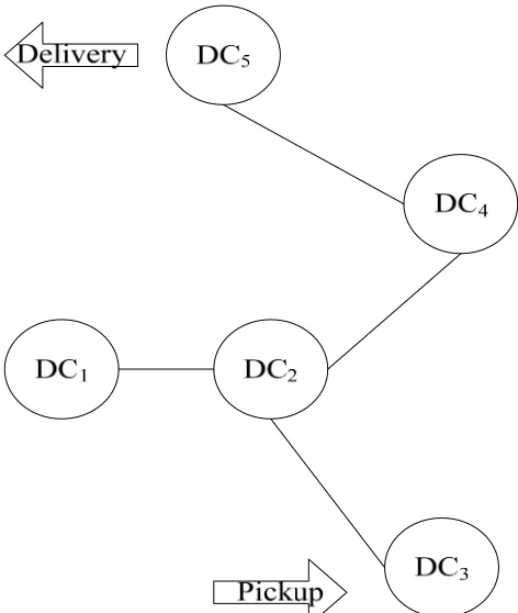
destination address. Figure 1.2 shows a package that enters at DC 3, travels to destination DC

4

Table 1.1 shows a comparison for functions of components in a PLN and the Internet [3].

DCs function like routers in the Internet. Packages transmitted by trucks are like data packets

transmitted by cables in the Internet.

Table 1.1. Comparison between Components of a PLN and the Internet

PLN Internet

Distribution Centers (DC)

Routers

Packages (Parcels)

Data Packets

5

1.3

Literature Review

Kay and Parlikad [2] analyzed material flow features in a PLN and compared three different

networks in terms of package average travel time. Bansal [5] studied PLN configurations and

proposed three mechanism to design a PLN. Kay [1] and Jain [3] proposed protocols for the

entities in the PLN to comply with. Those protocols make the PLN operate efficiently. In

their research, the average waiting time for a package is estimated to be the product of the

truck headway, which is the average interarrival time for trucks, and the headway ratio,

which is the assumed to have the value 0.5. As explained in the rest of this dissertation,

assuming a headway ratio of 0.5 is incorrect and yields inaccurate estimates of the

performance of a PLN.

1.4

Research Objectives

The main objectives of this research are to do the following:

1.

Develop a simulation model that builds on previous work of John Telford [6] to study

PLN operations. A PLN can be viewed as a priority queuing network with bulk

arrivals and bulk service. Due to the complexity of this problem, it is very difficult to

obtain a closed-form solution for package average waiting time. Therefore, a

simulation model is created in order to gain some insight and obtain some statistics on

the PLN operation, such as package average waiting time and the truck load factor

(that is, the space utilization for each truck trip, which is assumed to be the same for

6

2.

Use analytical and simulation models to find an accurate and practical procedure to

estimate package average waiting time. Kingman’s equation [7] is applied to

approximate the package average waiting time. The latter quantity can be represented

as the product of the truck headway and the headway ratio (refer to Section 2.2 for the

definition of this term). Statistics from the simulation and analytical models are then

used to estimate the headway ratio.

3.

Design the optimal PLN that yields minimal package average waiting times for all

packages’ origins and destinations. Potential locations (search space) for the DCs are

found using the U.S. network of interstate and highways. A genetic algorithm (GA) is

applied to the search space to determine the optimal number of DCs, their locations,

and the direct arc connections between adjacent DCs.

In addition to the main research objectives, we also discuss using the PLN simulation to

implement the protocols proposed in Kay [1] and Jain [3]. As an extension to the basic

simulation for the PLN, those advanced features focus on protocols, package bidding

procedures, truck agent behaviors, etc. A series of protocols have been developed by Kay [1]

for entities in the PLN to comply with. Packages bid for their transportation along the way.

Higher bidders get higher priority for truck transport services. Trucks obey a greedy rule, in

that they will transport the load of packages with the highest total bid. The bidding process

7

1.5

Layout of the Dissertation

Chapter 2 introduces the analytical and simulation models. We illustrate how the truck

headway and the headway ratio are used in the package average waiting time calculation.

Validation of the simulation model is presented as well.

Chapter 3 focuses on obtaining the package average waiting time approximation by

Kingman’s equation. Some statistics, such as the coefficient of variation for package

interarrival time, and the coefficient of variation for truck interarrival time, etc., are collected

from analytical and simulation models (with a simple package bidding scheme) and are used

in a regression-based method to estimate the headway ratio.

Chapter 4 presents the PLN simulation with some advanced features, including the package

bidding and truck acceptance of package loads. In addition, some of the simulation

architecture design issues are discussed.

Using results from Chapter 3, we present in Chapter 5 a procedure to design the PLN that

yields the minimal package average waiting time. A genetic algorithm is applied to search for

the number of DCs and their locations based on the U.S. network of interstate and highways.

8

2

PLN Analytical Model and Simulation Model

2.1

Literature Review

A computer simulation is a computer program that attempts to simulate an abstract model of

a particular system. Computer simulations have become a useful part of mathematical

modeling of many natural systems to gain insight into the operation of those systems, or to

observe their behavior [8, 9, 10]. Sadoun [11] provides a comprehensive review for applied

system simulation.

2.2

Headway and Headway Ratio for Waiting Time Calculation

Queuing theory has been widely used in practice to study average queue length, average

waiting time for a unit to receive service, etc. In the waiting time approximation, the service

time plays a big role. Actually, from the simple M/M/1 queue to the fairly complicated G/G/1

queue, expected waiting time is calculated as:

*

W

= θ μ

, (2.1)

where

μ

is the average service time and

θ

is a number determined by server utilization, job

arrival rate, and machine service rate. Different types of queuing systems have different

representations for

θ

. For example, for an M/M/1 queue,

θ

=

ρ

/(1-

ρ

) (where

ρ

is server

utilization); and for a G/G/1 queue,

θ

=

2 2

1

2

A B

C

C

ρ

ρ

⎛

⎞

⎛

⎞

+

⎜

⎟

⎜

₋

⎟

⎝

⎠⎝

⎠

, where

ρ

is the server utilization,

2 A

9

coefficient of variation of the service time. In Equation (2.1), the average waiting time for a

unit to receive service is expressed as the product of average service time (µ) and a number

(

θ

). In a PLN, the service time for package transportation is the truck interarrival time. This

suggests that, in a PLN, the package average waiting time can be approximated as the

product of truck headway (truck average interarrival time, which represents average service

time in a PLN) and the truck headway ratio, which is a term similar to

θ

in Equation (2.1),

consolidating all parameters except truck headway in the waiting time approximation

equation (for detailed queuing abstraction and model specification, refer to Section 3.2.1).

A simple example of this is as follows. If three trucks visit a station in 24 hours, then the

average truck headway is 8 hours. If the headway ratio is 0.5, then packages wait on average

four hours for a truck. Again, for different types of queues, the headway ratio has different

values.

The queuing principle that Poisson Arrivals See Time Averages (PASTA) states when the

arrival process to a system is Poisson, the long-run fraction of arrivals that see the process in

a particular state is equal to the long-run fraction of the time the process is in that state [12].

It is well known that, compared with the single-arrival, and single-service queuing model,

bulk features (bulk arrivals or/and bulk services) introduce more uncertainty and make the

average waiting time longer [15]. Without further research on package average waiting time

10

be less than one (if a random variable is exponentially distributed, its coefficient of variation

is 1). But it turns out that in a PLN, the headway ratio is much larger than 1, due to the

uncertainty induced by the bulk arrivals and bulk service as described above.

2.3

Analytical Model

Simulation is a good tool to study real-world problems. However, it is not always possible to

get insight into the system’s behavior solely by analyzing the output of a simulation of the

target system. Moreover, simulation is computationally intensive. Therefore, an approximate

analytical model has been developed and coded in MATLAB. This analytical model

calculates the number of trucks needed to handle a specific package demand, which can be

used as an input parameter in a simulation model to target a desired truck load factor.

In a PLN, the transport time for a package traveling from DC

to DC

is composed of three

parts: the time waiting for a truck (WT

), the loading and unloading time at each DC

(TimeLU, it is assumed to be the same in all DCs), and the actual travel time onboard a truck

(TT

):

WT + TT + TimeLU.

ij ij ij

t

=

(2.2)

Since the loading and unloading time and the travel time are fixed (assuming trucks travel at

a constant speed and packages are routed along the shortest paths), the only part left to

11

2.3.1

Analytical Model Assumptions

1.

Trucks operate around the clock and travel at constant speed.

2.

The truck load factor (which is defined to be the fraction of the truck’s capacity to

carry packages that is used on each trip) is 80%.

3.

The headway and headway ratio are used to approximate package average waiting

time as the product of the truck headway and the headway ratio.

2.3.2

Analytical Model Input Parameters

TimeLU: Loading and unloading time within DC (unit: minutes);

ProxFac: Proximity factor [2] (unit: none);

Nopkg: Total number of packages entering the PLN over a 24-hour period (unit: packages);

TrCap: Truck capacity (unit: packages);

TrSpeed: Truck traveling speed (unit: miles per hour);

LdFacA: Load factor for trucks (unit: none);

HWRatio: Headway ratio (unit: none).

The Proximity factor (ProxFac) represents the degree to which a DC is more likely to

12

information about the proximity factor can be found in Kay [2]. The quantity Nopkg is

assumed to be constant in the analytical model. The symbol arc

represents the direct

connection from DC

to DC

Similarly, the symbol arc

represents the direct connection from

DC

to DC

. We assume the direct connections between DCs are symmetric, that means if

arc

exists, then arc

exists as well, and vice versa. Note that if there is no direct connection

between DC

to DC

, then arc

and arc

do not exist.

2.3.3

Analytical Model Detailed Calculation

In the analytical model, analysis is focused on each individual arc (the direct connection

between two DCs). On each arc we calculate truck headway, package average waiting time,

and the number of trucks needed to meet the package demand.

In the analytical model, a number of packages (Nopkg) are transported by trucks in 24 hours.

The number of packages originating in a DC is determined by the population weight for the

area covered by that DC (as calculated in Equation (2.3)). The number of packages traveling

from an origin DC to a destination DC is proportional to the product of the population

weights for the origin and destination DCs (as explained in Section 2.3.3.1). For each specific

arc, the analytical model calculates how many truck trips are needed to meet the package

demand. Then the truck headway for that arc is the ratio of 24 to the number of truck trips on

that arc. The package average waiting time is calculated as the product of the truck headway

and the headway ratio. Since each truck travels at a constant speed, the package’s travel time

13

the PLN can be calculated by Equation (2.2). Finally, the number of trucks needed is the ratio

of the total truck hours (summing up the total travel time for each truck) to 24.

2.3.3.1 Number of Packages Transported between Two DCs

In the analytical model, the DC population weights are represented by a 36-element vector.

(We use Figure 1.1 as the PLN network where there are 36 DCs. Their locations and the

population each DC covers are known). The population weight of DC

,

wi

, is calculated in

Equation (2.3),

36

1

Pop

1, 2,...,36,

Pop

i i

j j

w

i

=

=

=

∑

(2.3)

where Pop

is the population covered by DC

.

The number of packages originating at each DC is proportional to its population weight,

nopkg_DC

=

nopkg * ,

w

(2.4)

The number of packages originating at DC

is the product of Nopkg and

w

.

The total number of packages (

nopkg_OD

) that travel from DC

to DC

is calculated as:

,

nopkg_OD

=

Nopkg * .

w

(2.5)

For a proximity factor equal to zero (ProxFac = 0),

*

.

ij i j

14

For none-zero proximity factor (ProxFac

≠

0), refer to Kay [2] for details on how to calculate

wij

.

Similarly, the total number of packages (

nopkg_OD

) that travel from DC

to DC

is

calculated as:

,

nopkg_OD

=

nopkg *

w

.

(2.7)

Since

w

=

w

=

w

*

w

, the quantity

nopkg_OD

is the same with the quantity

,

nopkg_OD

.

2.3.3.2 Number of Packages Transported on a Single Arc

The number of packages traveling over the arc from DC

to DC

is represented by

,

nopkg_arc

. Similarly, the number of packages traveling over the arc from DC

to DC

is

represented by

nopkg_arc

. Dijkstra's algorithm [13] is used to find out the shortest path

from any DC to another.

The following example explains the difference between

nopkg_OD

and

nopkg_arc

. In

the PLN shown in Figure 2.1, the solid lines represent arcs between two DCs, and the dotted

lines represent packages transported from one DC to another. The quantity

nopkg_OD

represents the number of packages traveling from DC

to DC

and the shortest path for those

packages requires travelling through arc

, and arc

. The quantity

nopkg_OD represents

15

requires travelling over arc

. The quantity

nopkg_OD represents the number of packages

traveling from DC

to DC

, and the shortest path for those packages requirs travelling

through arc

, and arc

.

The quantity

nopkg_arc represents the number of packages going through

arc . In the

example given above, the quantity

nopkg_arc is the summation of the quantities

3,2

nopkg_OD ,

nopkg_OD and

nopkg_OD since all of those packages go through

arc .

Note that, as explained in Section 2.3.2, the symbol arc

represents the direct connection

from DC

to DC

. But if there is no direct connection between DC

to DC

, then arc

does not

exist and the quantity

nopkg_arc

is not defined. For example in Figure 2.1, the symbol

arc

does not exist since there is no direct connection between DC

and DC

. Therefore, the

quantity

nopkg_arc is not defined. However,

nopkg_OD is defined as the number of

packages traveling from DC

to DC

. This shows the difference between

nopkg_OD

and

16

Thus, the quantity

nopkg_arc

is the total number of packages whose shortest path goes

through

arc

,

nopkg

, 1

nopkg_arc

(pkg goes through the arc from DC to DC ),

I

k

=

=

∑

(2.8)

where

I

(·) is an indication function,

1, if condition is true,

(condition)

0, if condition is false.

I

= ⎨

⎧

17

2.3.3.3 Truck Headway

Since we assume trucks operate around the clock, the truck headway is calculated as follows:

,

,

24

Headway ,

nopkg_arc / (TrCap * LdFacA)

i j

=

(2.10)

where TrCap*LdFacA represents how many packages each truck trip transports, and

,

nopkg_arc / (TrCap*LdFacA)

represents how many truck trips are needed on arc

to meet

the demand.

2.3.3.4 Number of Trucks in the PLN

The number of trucks needed is calculated as follows:

nopkg

1

/ (TrCap*LdFacA)

notruck

,

24

k

t

⎡

⎤

⎢

⎥

⎢

⎥

=

⎢

⎥

⎢

⎥

⎢

⎥

∑

(2.11)

where

t

is the total truck transport time of

k

th package. Notice that this does not include

package waiting for truck time and loading and unloading time at DCs.

2.3.4

The Outputs from the Analytical Model

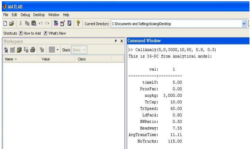
To give an example of output from the analytical model, we run the analytical model with

following parameter values, TimeLU=5, ProxFac=0, Nopkg=3000, TrCap=10, TrSpeed=60,

18

load factor, 115 trucks are needed in the simulation. This number of trucks serves as one

input parameter into the simulation model to achieve the same load factor level.

Figure 2.2. Output Snapshot from the Analytical Model

2.4

Simulation Model

The simulation model is developed using Microsoft .NET framework to take advantage of its

advanced data structures and efficient program control procedures [14]. Under the .NET

platform, every entity is implemented as an object [14]. This simulation model is based on

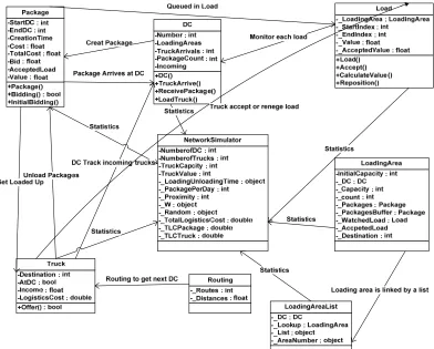
Telford’s logistics simulation library [6]. In Figure 2.3, each object is enclosed in a rectangle

along with its properties, operations, etc. For example, each package is an object and has

properties StartDC and EndDC, as well as several associated functions (e.g.,

Package

).

19

2.4.1

Simulation Model Detailed Description

2.4.1.1 Simulation Initialization

The simulation program runs 25 replications, and 3,600 days for each replication. The

initialization function initializes the simulation program. The initialization function generates

the event calendar, loads the input data sets, and calls functions to create DCs, loading areas,

20

waiting times, truck load factors, etc. Finally, it schedules the simulation termination events

onto the event calendar to finish the simulation when the termination condition is met.

2.4.1.2 Load Input Data Sets

The analytical model generates text files to hold the following information: distance between

any two DCs (

Distances

), a matrix representing the direct arc between two DCs

(

ArcDistance

), and the package routing scheme (

Routing

), which is determined using

Dijkstra’s algorithm [13]. The LoadData function loads this information to be used in

simulation.

2.4.1.3 Package Generation

The total number of packages generated in the simulation is 1.8 million per day, which is

approximately the same number of packages handled daily by UPS in the southeastern

U.S.A. [2]. Packages are generated according to a Poisson process. Like the analytical model,

the number of packages originating in a particular DC is proportional to its population

weight. When a package is generated, its origin DC and destination DC are randomly

generated based on the DCs’ population weights. At the same time, the count for total

number of packages generated in the simulation (

PackageID

) is incremented by one.

2.4.1.4 Package Routing

Whenever a package reaches a DC, the

Routing

function is called to determine its next DC

21

package’s destination DC, then the current package is eliminated from the simulation and

some statistics, such as PackagesDelivered, PackageWaitTime, etc. are updated. If the

current DC is not this package’s destination, then the package is put in the package queue

(loading area) to wait for a truck to transport the package to its next destination.

2.4.1.5 DC Services

DCs play a central role in the PLN operation. A DC collects packages originating from the

local areas it covers, maintains package queues, provides related information for incoming

trucks and packages, etc. Each DC has a loading area (package queue), for each immediately

adjacent DC, i.e., each DC that shares a direct arc connection. For example, in Figure 2.4,

DC

is adjacent to DC

, DC

, and DC

. Then, within DC

, there are three loading areas

designated for packages heading to DC

, DC

, and DC

. Whenever a package reaches a DC,

if this is not its destination DC, then the package is placed in the loading area that

22

When a truck arrives at a DC, the

ReceivePackage

function is called to perform the following

operations: (i) empty the arriving truck; (ii) call function

Routing

to route each package on

that truck to its next DC by putting the package in the corresponding loading area (if this is

the final destination DC for a package, this package is eliminated from the simulation); and

(iii) update all the related statistics.

In order to attract trucks to come to a DC and transport packages, only trucks currently at this

DC and trucks heading to this DC from other DCs directly connected with this one are made

eligible to accept a load of packages (that is, eligible for the load offering process). For

23

is heading to DC

, which is adjacent to DC

, and truck 3 is currently at DC

. In this scenario,

only truck 1 and truck 3 are eligible for this load offering. Since truck 3 is currently at DC

,

truck 3 has higher priority than truck 1; and thus truck 3 will be the first truck to have the

chance to consider accepting this load. Note truck 2 is heading to DC

not DC

, so truck 2 is

not eligible for the load offering at DC

24

2.4.1.6 Trucks

The analytical model calculates the number of trucks that are needed to achieve the target of

an 80% truck load factor on each arc on the average. In the initialization process, the initial

locations of all trucks are randomly generated. That means, unlike packages, all trucks enter

the simulation at one time. Once packages enter the simulation, trucks start to accept

packages, load the accepted packages, and travel to their next DC.

2.4.1.7 Loading Areas

Within a given DC, each loading area is a queue to hold packages waiting for transport to a

specific DC. When packages come into a DC and are routed to the next DC, a function

named

Add

is called to add those packages to the corresponding loading area. The first

L

packages (where 0<

L

<=TrCap*LdFacA) comprise a load (named

watchload

). The loading

areas in a DC take turns to offer their

watchload

to trucks. If a truck accepts that

watchload

,

then a function named

LoadTruck

is called to perform the following operations: (i) move this

load of packages onto the truck; and (ii) arrange for the truck to leave for the next DC

immediately by making a call to function

TruckAccepted

.

2.4.1.8 Statistics Objects

A number of statistics objects, such as

ArcPackageIntArrMean

,

ArcTrucksLastArr

,

25

2.4.1.9 Simulation Termination

When the simulation time reaches the preset limit, a function named

Terminate

is called to

terminate the simulation program. The function

Terminate

destroys all objects, releases

computer memory, and creates text files with designated statistical outputs.

2.4.2

Simulation Model Input Parameters

TimeLU: Loading and unloading time within a DC (unit: minutes);

ProxFac: Proximity factor (unit: note);

Nopkg: Total number of packages entering the PLN over a 24-hour period (unit: packages);

TrCap: Ttruck capacity (unit: packages per truck);

TrSpeed: Truck traveling speed (units: miles per hour);

NoTrucks: Number of trucks in the PLN (unit: trucks).

26

2.4.3

Simulation Outputs

Figure 2.6. Output Snapshot from the Simulation Model

Figure 2.6 shows that with the current set of parameters (TimeLU = 5, ProxFac = 0, Nopkg =

3000, TrCap = 10, TrSpeed = 60, LdFacA = 0.8), the load factor is 82%. The average transit

time for packages is 17.96 hours, and the package average wait time is 10.34 hours.

2.5

Simulation Model Validation

Before further research is carried out with the simulation model, it is necessary to validate

that it is working correctly. Little’s law [15] calculation and M/G/1 queuing calculation are

used to validate the simulation model.

Little’s Law: The long-run average number of customers in a stable system (over some time

interval), WIP, is equal to the long-run average arrival rate of customers,

λ

, multiplied by the

long-run average cycle time in the system, CT [15]:

WIP

=

λ

CT.

(2.12)

In the simulation, WIP is the average number of total packages waiting in queues and the

27

average arrival rate of packages, and CT is the average length of time a package stays in the

PLN. The simulation model keeps track of the total number of packages created and each

package’s cycle time. The long-run average arrival rate of customers is the ratio of the total

number of packages created to the simulation length. The long-run average cycle time is the

average of recorded package’s cycle time in the simulation. The value of WIP (denoted by

WIP_Calc) is calculated as the the product of the long-run average arrival rate of customers

and the long-run average cycle time. The simulation model aslo keeps track of package

queue length. The estimated WIP value (denoted by WIP_Simu) is the average number of

packages in the PLN. The validation is to see how much difference is between WIP_Simu

and WIP_Calc.

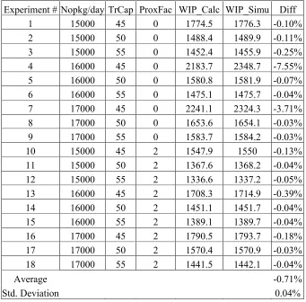
The simulation program runs 25 replications, and 3,600 days for each replication. The

simulation wamp-up period is 90 days. Based on a 36-DC PLN (shown in Figure 1.1),

eighteen different parameter sets were used in the simulation model. TimeLU (loading and

unloading time of 5 minutes), and TrSpeed (truck speed of 60 mph), were kept the same

28

Experiment # Nopkg/day TrCap ProxFac WIP_Calc WIP_Simu Diff 1 15000 45 0 1774.5 1776.3 -0.10% 2 15000 50 0 1488.4 1489.9 -0.11% 3 15000 55 0 1452.4 1455.9 -0.25% 4 16000 45 0 2183.7 2348.7 -7.55% 5 16000 50 0 1580.8 1581.9 -0.07% 6 16000 55 0 1475.1 1475.7 -0.04% 7 17000 45 0 2241.1 2324.3 -3.71% 8 17000 50 0 1653.6 1654.1 -0.03% 9 17000 55 0 1583.7 1584.2 -0.03% 10 15000 45 2 1547.9 1550 -0.13% 11 15000 50 2 1367.6 1368.2 -0.04% 12 15000 55 2 1336.6 1337.2 -0.05% 13 16000 45 2 1708.3 1714.9 -0.39% 14 16000 50 2 1451.1 1451.7 -0.04% 15 16000 55 2 1389.1 1389.7 -0.04% 16 17000 45 2 1790.5 1793.7 -0.18% 17 17000 50 2 1570.4 1570.9 -0.03% 18 17000 55 2 1441.5 1442.1 -0.04%

Average -0.71% Std. Deviation 0.04%

As shown in Table 2.1, the average difference between the WIP value recorded in the

simulation and the theoretical WIP value is –0.71% (with a standard deviation of 0.04%, and

a 95% confidence interval of (–1.24% , –0.64%)).

In the PLN, if the truck capacity is constrained to be one and the packages arrival process is

Poisson distribution, then the PLN network reduces to a M/G/1 queuing model. The

Pollaczek-Khinchin formula [16] is used to calculate the long-run package average waiting

29

The package average waiting time ( ˆ

W

) is computed as,

2 eff

eff

1

ˆ

_,

1

2

B

q B

C

W

ρ

μ

ρ

⎛

⎞⎛

+

⎞

= ⎜

₋

⎟⎜

⎟

⎝

⎠

⎝

⎠

(2.13)

where

ρ

is the effective server utilization,

C

is the squared coeffient of variation for the

truck headway (time between the (

k

-1)st truck and

k

th truck to arrive at DC

with DC

as the

next destination) and

μ

is the mean value for the truck headway. Refer to Section 3.2.2.1

for detailed notation and definition. Note that since the package arrival process has a Poisson

distribution, the squared coeffient of variation for the package interarrival time is one.

The simulation program runs 25 replications, and 3,600 days for each replication. The

simulation wamp-up period is 90 days. Based on a 3-DC PLN, in the simulation model,

packages arrive according to a Poisson process (different numbers of packages for the PLN

are used for multiple experiments), the truck capacity is one, and the loading and unloading

time is 5 minutes. In the simulation, we record the squared coeffient of variation for the truck

headway (

C

), the mean value for the truck headway (

μ

), and the package average waiting

time (

W

). The quantity

ρ

is 80% (refer to Section 3.2.2.4 for a detailed discussion for the

effective server utilization) and then ˆ

W

is estimated by Equation (2.13). The comparison

between the package average waiting time in the simulation (

W

) and the estimated package

30

Experiment # Nopkg/day WT_Simu (

W

)

W

ˆ

)

1 150 9.1 8.2 10.3%

2 160 9.1 8.3 8.5%

3 170 9.6 9.1 5.4%

4 180 9.7 9.5 1.8%

5 190 9.9 10.1 –1.6%

6 200 10.5 10.9 –3.8%

Average 3.4%

Std. Deviation 5.6%

On average, the difference between the package average waiting time recorded in simulation

(

is 3.4% (with a standard

31

3

Package Average Waiting Time Approximation

3.1

Literature Review and Research Issues

Kay and Parlikad [2] analyzed material flow features in a PLN. Bansal [5] studied PLN

configuration and proposed some mechanisms to design a PLN. Kay [1] and Jain [3,3]

proposed some protocols (for package bidding, truck agent behavior, etc) for the PLN, and

they tried to make the PLN work more efficiently. In their research, the average waiting time

for a package is based on truck headway, which is the interarrival time for a truck at a DC.

Average waiting time is assumed to be half of the headway (headway ratio is 0.5).

In the PLN network design problem, the package average waiting time is critical since it is a

large component of the measurements to evaluate each proposed network configuration.

Therefore, a better approximation for package average waiting time is needed to revise and

refine a model of the performance of a PLN network.

A simulation model [8] has been built to observe the values of performance metrics that are

needed in the package average waiting time approximation. Those values cannot be obtained

by exact queuing-theoretic analysis due to the complexity of the PLN (a priority queuing

network with bulk arrivals and bulk service).

Bulk service queuing problems in transportation have attracted many researchers and

scholars since the mid-twentieth century. The original paper in this field was published by

32

number of waiting customers. Since then, a large number of contributions have been made to

the field, including Downton [18] Miller [19], Neuts [20], Cohen [21], Chaudhry [22] and

Powell [23, 24, 25]. Downton formally analyzed the average waiting time problem with bulk

arrivals and bulk service, which laid a solid groundwork for future research on this problem.

Neuts researched bulk queues with different vehicle-control strategies, but he only

considered a single Poisson arrival stream. Powell studied this research issue from the

perspective of load planning. He also approximated the average waiting time with iterative

numerical computing. However, his work is heavily dependent on his specific model and

vehicle-control policies. Tegiilm [26] and Borthakur [27] considered the general bulk service

rule for bulk arrivals (with variable sizes for arrivals).

Whitt [28, 29] studied limiting theorems in the condition of heavy traffic. He also studied an

interpolation approximation for the mean workload in a GI/G/ 1 queue. However, this does

not apply to the bulk-arrival and bulk-service scenario. Marchal [30] developed some simple

waiting-time approximations for the GI/G/1 and GI/G/c queues. Kingman [7] developed an

approximation for the average waiting time for the GI/G/1 queue. Kingman’s approximation

has been used by Hopp [15], who showed that when server utilization is high, the

33

3.2

Package Average Waiting Time Approximation in a PLN

3.2.1

The PLN Queuing Model Abstraction

Figure 3.1 shows the abstraction of the PLN to a standard queuing model. In a PLN, any arc

(direct connection) between two DCs contains a package queue. The arc between DC

and

DC

contains two package queues: one queue with packages going from DC

to DC

, and

another queue with packages going from DC

to DC

A truck transports a load of packages

on each trip between two DCs, and when the truck reaches a DC, its load of packages are

disassembled, and the associated packages are moved to their assigned package queues.

Clearly, the PLN operation involves bulk arrivals and bulk service. A PLN is an open

interconnected network of such package queues. So a PLN can be abstracted as an open

queuing network with bulk arrivals and bulk service.

The package waiting time for truck transport is composed of two parts. In part 1 of the

waiting process, packages form a load in the assembly queue. In part 2 of the waiting

process, loads waiting in the transport queue for shipment to their next destination DC. When

packages arrive at a DC, they are put in the appropriate assembly queue. Whenever a number

of packages (

L

packages, where

L

is the load size) form a load, this load is immediately

moved to the transport queue to wait for truck transport. On each trip, a truck only transports

one load to the destination DC. If customers in the system are loads, then the system can be

modeled as a network of interconnected G/G/1 queues. The customers’ arrival process is

34

the time between the formation of consecutive loads. The service is defined as truck

transport, and the service time is the interarrival time between consecutive trucks destined for

the same DC. Detailed definition can be found in Section 3.2.2.1.

35

3.2.2

Mathematical Formulation of Target Problem

3.2.2.1 Definitions

The following definitions and terms apply to the package waiting time approximation.

Service: truck trip from one DC to another

Headway: interarrival time between consecutive trucks arriving at DC

that are

destined for DC

Average load size:

L

packages

k

U

: Time between arrival of package

k

–1 and package

k

at the assembly queue

of packages at DC

waiting for transport to DC

.

u

μ

: Mean value of

U

u

σ

: Standard deviation of

U

u

C

: CV (coefficient of variation) of

U

,

u

C

σ

μ

=

Ak

: Time between the formation of load

k

–1 and load

k

in the queue of loads at

DC

waiting for transport to DC

.

A

μ

: Mean value of

A

A

σ

: Standard deviation of

Ak

A

C

: CV of

Ak

C

σ

36

B

: Headway, time between the arrival of the (

k

– 1)st truck and

k

th trucks at one

DC

with the same next destination.

B

μ

: Mean value of

Bk

B

σ

: Standard deviation of

Bk

B

C

: CV of

Bk

C

σ

μ

=

A

r

: Arrival rate of loads at one DC waiting for transport to the same next DC:

1/

A A

r

=

μ

B

r

: Rate at which trucks arrive to pick up a load from the queue of loads waiting

at DC

for transport to DC

: 1/

r

=

μ

ρ

: Truck (server) utilization:

B A

r

r

μ

ρ

μ

=

=

Since a load is composed of

L

packages (

( 1) 1 kL

k j

j k L

A

U

= − +

=

∑

), we have

μ

=

L

μ

, and

2 2

A

L

σ

=

σ

. Substituting in these values, we can see that

2 2 2

2 2

2

₍

₎

u u u

A A

A u u

L

C

C

L

L

L

=

σ

=

σ

=

σ

=

μ

μ

μ

.

3.2.2.2 Average Waiting Time for a Load

Consider a load at DC

waiting to be transported to DC

. Based on the average waiting time

37

2 2

ˆ

1

2

A B

q B

C

C

W

ρ

μ

ρ

⎛

⎞

⎛

⎞

+

=

_⎜

_⎟

_⎜

_⎟

−

⎝

⎠⎝

⎠

(3.1)

where

ρ

is truck utilization,

C

is the squared coefficient of variation for load interarrival

time,

C

is the squared coefficient of variation for trucks interarrival time (headway), and

B

μ

is the headway mean value.

Within a PLN, since the package arrival process is not a Poisson process due to the batch

arrival of packages on trucks to a DC and the service time (truck headway) is not

exponentially distributed, values for

ρ

,

C

and

C

can only be observed from the

simulation. The headway mean value

μ

can be obtained by the analytical model (described

in Section 2.3), given the demand rates at each DC and the truck capacity.

3.2.2.3 Average Waiting Time for a Package

In a PLN, when a package arrives, it is put in the assembly queue to wait for a load to be

formed. After a load is formed, it is put into a transport queue, where it waits for truck

transportation.

Suppose a package is currently in DC

, and it is going to DC

. The average waiting time for

this package consists of two parts:

(i)

The time spent waiting in an

“

assembly queue

”

until a

“

complete

”

38

truckload immediately exits the assembly queue and joins the “transport

queue,” which is a queue of truckloads waiting for a truck that will

transport the first waiting truckload from DC

to DC

;

(ii)

The time spent in the

“

transport queue

”

until a truck destined for DC

finally arrives at DC

so that the first waiting truckload can exit the

transport queue and start the trip to DC

.

The “service time” in the transport queue is taken to be the headway (delay) between the

arrival of successive trucks that are destined to deliver a truckload to DC

, and where it is

assumed that the transport queue is rarely empty.

Let

X

denote the waiting time of the target package in the assembly queue. If the target

package is the th

k

package to be added to the truckload currently being assembled

for

k

=

1, , 1

…

L

−

, then for

l

= +

1, ,

k

…

L

, let

U

denote the interarrival time between the

l

th package and the

(

l

−

1)st

package in the same truckload so that the total waiting time in the

assembly queue for the target package is

1

0,

if

,

, if

1,...,

1.

k

l l k

k

L

X

U

k

L

= +

=

⎧

⎪

= ⎨

₌

₋

⎪⎩

∑

(3.2)

39

0,

if

[

]

(

)

for 1,..., .

[ ], if

1,...,

1

k U

l l k

k

L

E X

L k

k

L

E U

k

L

μ

= +

=

⎧

⎫

⎪

⎪

=

_⎨

_⎬

=

−

=

=

−

⎪

⎪

⎩

∑

⎭

(3.3)

The operation of assembling each truckload is defined as a renewal-reward process in which

a renewal epoch occurs each time the assembly of another truckload is finally completed,

therefore a standard renewal-reward argument can be used to prove the intuitively obvious

result that the long-run average time spent by the target package in the assembly queue is

assem 1

1

[

].

W

E X

L

=

∑

(3.4)

From Equations (3.3) and (3.4), the long-run average waiting time for a package in the

assembly queue is

assem 1

1

(

)

W

L

k

L

μ

=

∑

−

(3.5)

1 1 L U v

v

L

μ

=

∑

(3.6)

(

1

)

2

U

L

L

L

μ

⎡

−

⎤

=

_⎢

_⎥

⎣

⎦

(3.7)

(

1)

.

2

U

L

μ

−

=

(3.8)