DOI: 10.1534/genetics.107.080820
Multivariate
Q
st–
Fst
Comparisons: A Neutrality Test for the Evolution of
the G Matrix in Structured Populations
Guillaume Martin,*
,†,1Elodie Chapuis*
,‡and Je´ro
ˆme Goudet*
*De´partement d’Ecologie et Evolution, Universite´ de Lausanne, CH 1015 Lausanne, Switzerland,†Ge´ne´tique et Evolution des Maladies Infectieuses, UMR 2724, IRD, 34394 Montpellier Cedex 5, France and‡Institut des Sciences
de l’E´volution, UMR 5554, Universite´ Montpellier II, 34095 Montpellier Cedex 5, France Manuscript received August 20, 2007
Accepted for publication November 18, 2007
ABSTRACT
Neutrality tests in quantitative genetics provide a statistical framework for the detection of selection on polygenic traits in wild populations. However, the existing method based on comparisons of divergence at neutral markers and quantitative traits (Qst–Fst) suffers from several limitations that hinder a clear interpretation of the results with typical empirical designs. In this article, we propose a multivariate extension of this neutrality test based on empirical estimates of the among-populations (D) and within-populations (G) covariance matrices by MANOVA. A simple pattern is expected under neutrality:D¼ 2Fst/(1Fst)G, so that neutrality implies both proportionality of the two matrices and a specific value of the proportionality coefficient. This pattern is tested using Flury’s framework for matrix comparison [common principal-component (CPC) analysis], a well-known tool inGmatrix evolution studies. We show the importance of using a Bartlett adjustment of the test for the small sample sizes typically found in empirical studies. We propose a dual test: (i) that the proportionality coefficient is not different from its neutral expectation [2Fst/(1 Fst)] and (ii) that the MANOVA estimates of mean square matrices between and among populations are proportional. These two tests combined provide a more stringent test for neutrality than the classic Qst–Fst comparison and avoid several statistical problems. Extensive simulations of realistic empirical designs suggest that these tests correctly detect the expected pattern under neutrality and have enough power to efficiently detect mild to strong selection (homogeneous, heterogeneous, or mixed) when it is occurring on a set of traits. This method also provides a rigorous and quantitative framework for disentangling the effects of different selection regimes and of drift on the evolution of theGmatrix. We discuss practical requirements for the proper application of our test in empirical studies and potential extensions.
T
HE comparison of genetic differentiation at neutral markers and at quantitative traits is a commonly used method to estimate the relative impacts of drift and selection on polygenic traits in the wild. Typically, a set of populations is sampled, from which the differentiation among populations is estimated for a set of molecular markers (Fst) and is compared to the same measure ofdifferentiation at a single or a set of quantitative traits (Qst). Under pure neutrality, and if the traits are additive,
Qst¼Fstfor any trait (Spitze1993). Departures from this
neutral expectation are considered evidence of selection acting on the quantitative trait under study.Qst,Fstis
evidence of homogeneous selection for the trait among populations,i.e., selection for the same optimal value of the trait in all populations, whileQst.Fstis evidence of
heterogeneous selection for the trait,i.e., selection for different optima among populations (Merila and
Crnokrak2001).
However, proper empirical detection of selection requires being able to detect a statistically significant
departure from the neutral expectation (Qst¼Fst) and
therefore depends on the confidence intervals (C.I.’s) of both QstandFstestimates. When studying single traits,
confidence intervals onQstare very large (Merilaand
Crnokrak2001; Latta2004; O’Haraand Merila2005;
Goudetand Buchi2006), often spanning.50% of their
total possible range [0, 1], even in the most recent studies with a large sampling effort (Porcher et al. 2006).
Furthermore, the methods employed to estimate the C.I. are not always statistically efficient (O’Hara and
Merila2005). Overall, the power of the test with single
traitsQstis very low with the sampling designs typically
possible in empirical studies (O’Haraand Merila2005),
so that rejection of the neutral expectation is unlikely, even when fairly strong selection is in fact occurring (Latta2004). Consequently, mostQst–Fstcomparisons
use mean Qstvalues among a set of quantitative traits,
which are compared toFstestimates from several marker
loci (Chapuiset al.2007). In doing so, the C.I. forQstis
reduced (and the power of the test increased) at the cost 1Corresponding author:Institut des Sciences de l’Evolution–Montpellier,
Unite´ Mixte de Recherche UMII–CNRS (UMR 5554), Universite´ de Montpellier II–CC 065, 34095 Montpellier Cedex 05, France.
E-mail: [email protected]
of losing information on individual traits. However, even with meanQstvalues, the C.I.’s obtained are often still
large (see,e.g., Merilaand Crnokrak2001).
Further-more, and maybe more importantly, the method used to compute the C.I. for the mean Qst often implicitly
assumes that the quantitative traits are mutually indepen-dent. This has two drawbacks: (i) in general the traits under scrutiny show some level of covariance within populations so that the resulting C.I. estimates may be unreliable, and (ii) the information contained in these covariances is not used in the analysis. Recent methods can partly correct for covariance between traits, but often not completely, and they are rarely applied in practice, maybe because of their statistical complexity. In addition, even when correctly estimated, the C.I.’s forQstremain
large (O’Haraand Merila2005). However, Kremeret al.
(1997) proposed a measure of Qst on several traits.
Although this method does not really use the information contained in covariances between traits, it does correct for these covariances to provide a (still univariate) measure ofQst(calledCQstby the authors). As expected,
when used by Waldmann and Andersson (1999) in
subdivided populations of two plant species, it provided smaller (and more reliable) C.I.’s in the measure ofQst
than previously observed on individual traits.
On the other hand, the study of multivariate pheno-typic distributions in the wild has led to a flourishing literature on the evolution of genetic covariances be-tween traits, summarized into the matrix of genetic covariances: theG matrix. Since Lande (1979)
intro-duced a multivariate framework to predict the evolution of a set of polygenic traits under selection and drift, the importance of genetic covariances in constraining adap-tive evolution has been a major focus of evolutionary biology (see a special issue of The Journal of Evo-lutionary Biology, Blows2007). Numerous studies have
sought to estimate theGmatrix in different species or in different populations of the same species, to test to what extentGmatrices could evolve under the influence of various evolutionary forces and how they could con-strain the evolutionary trajectory of natural populations (reviewed in Steppanet al.2002; McGuigan2006).
However, as for the case of single-quantitative-trait studies, disentangling the effects of selection and drift on multivariate covariances has proved difficult empir-ically (Steppanet al.2002). For this purpose, alternative
predictions on the pattern of multivariate phenotypic distributions among populations or species must be made according to whether drift or selection is the main driving force of the pattern. It was initially suggested thatGmatrices in distinct populations undergoing only drift should be proportional to each other, while this was not expected under selection (Roff 2000). However,
this prediction is in fact theoretically incorrect (Phillips
et al.2001):Gmatrices from individual populations can
differ largely even under the action of drift alone. It is only theaverageGamong many drifting populations
that is expected to be proportional toGin the ancestral population from which they are derived, and this ancestral population is rarely available to the experi-menter. This result was demonstrated empirically by Phillipset al.(2001).
In an influential study of morphological traits in stickleback fishes, Schluter(1996) compared thewithin
-populations covariances (G) with theamong-populations covariances (the divergence matrixD). He showed that the leading phenotypic axis of within-population vari-ance (the main eigenvector ofG) pointed in a similar direction to the main axis of population divergence (the leading eigenvector ofD). As this similarity tended to decay with the divergence time between species, he concluded that this pattern was evidence of the action of divergent selection between stickleback species. More recently, McGuigan et al. (2005) extended their
ap-proach to comparisons of whole matrices (G vs. D) instead of only leading eigenvectors. Unfortunately, as was pointed out by the authors, similarity betweenGand D can be generated by selection as well as by drift (Lande 1979) and therefore detecting this pattern
alone does not allow disentangling the two effects. In addition, tests of qualitative similarity between matrices may have low power (Steppanet al.2002), and, to our
knowledge, their statistical behavior has never been studied precisely.
More generally the problem that observable patterns inGcan be due to both selective and neutral processes has led to criticisms of the whole research program that seeks to useGmatrix estimates to get insights into the constraints imposed by evolutionary forces on pheno-typic evolution (Pigliucci 2006). Given the already
large designs required for evolutionary quantitative genetic studies, it seems that they are more likely to be improved through more appropriate statistical ap-proaches than by increased empirical efforts. In this article, we attempt to overcome these difficulties by devising a neutrality test on the basis of alternative expectations from neutralityvs.selection and by explic-itly checking its statistical properties by simulations. Our approach is to extend the classicQst–Fstcomparison to
multivariate phenotype distributions, by using the in-formation from neutral markers in comparisons of the GandDmatrices.
Rogers and Harpending (1983) proposed a
neu-trality test that is in fact a multivariate method to compareQstandFst, although it was not described in
those terms. The method accounts for nonindepen-dence between traits and de facto provides a clear quantitative expectation for the evolution of the G matrix under neutrality. Similar to a previous suggestion of Lande (1979), they suggested to compareGandD
and showed that the expected relationship between these two matrices under neutrality wasD¼2Fst/(1
Fst)G(Equation 16 of Rogersand Harpending1983).
in multivariate evolution, this suggestion has been somewhat overlooked in the empirical literature (but see Merila1997). This may stem from the fact that their
results were obtained in the limiting context of traits encoded by nonpleiotropic and diallelic loci and that the statistical behavior of the test they proposed was not studied in detail. Furthermore, the test compares only the value of the proportionality constant with its ex-pectation (2Fst/(1Fst)) but does not test for
propor-tionality ofGandDitself. Finally, no explicit statistical approach was proposed by the authors to implement this multivariate test.
The aims of this article are (i) to generalize the prediction on the relationship betweenGandDunder neutrality using results from coalescent theory, (ii) to use this prediction as a basis for a new neutrality test, and (iii) to check the statistical efficiency of our test by simulations of realistic empirical designs. An applica-tion of the test to empirical data is provided in an accompanying article (Chapuiset al.2008). Our
statis-tical test uses the general framework of sample co-variance matrix comparisons (Flury1988), also known
as common principal component (CPC) analysis. This method, which has been introduced in evolutionary biology by Phillipsand Arnold (1999), allows
deter-mining the level of shared structure among an arbitrary number of covariance matrices of arbitrary dimension. These matrices may be equal, be proportional, or have a number of principal components in common. To test our neutral expectation (further detailed below) requires testing for proportionality only between two matrices. The simplicity of this test (one of the simplest subcases of CPC analysis) provides a straightforward testing approach, whose statistical efficiency is evaluated through individual-based simulations.
METHODS
Multivariate neutrality test for additive traits:
Ex-pected pattern under neutrality:Consider a set of
popula-tions for which a set of quantitative traits undergoes only mutation and genetic drift, but no selection. The quantitative characters under study are assumed to be additive, and the loci underlying these characters are assumed to be at linkage equilibrium. The mean value of each trait is expected to diverge randomly across populations because of drift and mutation. Consider that the set of subpopulations diverged from a given common ancestral population. Using coalescent theory, Whitlock (1999) showed that the expected genetic
variance of any additive trait both within and among subpopulations can be expressed as a function of (i) the total mutational variance for that trait (s2
m), (ii) the
effective size (Ne), and (iii) Wright’s index of
popula-tion differentiapopula-tion (Fst) in the metapopulation.
Al-though originally expressed in terms of variances, the argument is also valid in the more general case of
covariances between any pair of traits (z1andz2), simply
by replacings2
mby the mutational covariance betweenz1
andz2due to pleiotropy (c12). The expected covariances
within and among populations (covw andcovb,
respec-tively) can thus be expressed as
covbðz1;z2Þ ¼4FstNec12
covwðz1;z2Þ ¼2ð1FstÞNec12 ð1Þ (from Equations 12 and 13 of Whitlock1999). Because
they are proportional to the same quantity Nec12, a
simple relation between the two covariances is deduced from Equation 1: covb(z1,z2)¼2Fst/(1Fst)covw(z1,z2)
for any pair (z1,z2). This relation can be expressed in
matrix form for a set of traits that are all neutral and additive (but not necessarily independent). IfE(D) and
E(G) are the expected among-populations and within-populations covariance matrices in the metapopulation, we expect
EðDÞ ¼ 2Fst 1Fst
EðGÞ: ð2Þ
For a haploid or a completely inbred diploid species, the factor 2 is dropped from the right-hand side of the equation. Furthermore, from Equation 4 of Whitlock
(1999), it appears that for a species with a significant level of inbreeding, the right-hand side of Equation 2 above should be divided by (1 1 Fis), where Fis, the
inbreeding coefficient within populations, is also esti-mated from the neutral markers.
Equation 2 is similar to Equation 16 of Rogersand
Harpending(1983), which was obtained in the limiting
case of a polygenic trait encoded by nonpleiotropic diallelic loci and developed in the context of the island model. In fact, the derivation of Equation 2 from coalescent theory shows that this result is valid whatever the forces shaping the neutral divergence among populations (e.g., isolation by distance, extinction– colonization, migration, etc.) and the number of alleles encoding the quantitative traits under focus. Therefore, it should be valid for any metapopulation undergoing neutral divergence and mutation, provided that the determinism of the traits is additive (as for the classic
Qst¼Fstexpectation). The main limitations inherent in
the coalescent approach used here are that linkage disequilibrium between quantitative trait loci should be small and that mutational variance per generation on each trait should be independent of the current state of the population (Whitlock1999). Note that under
the specific scenario of population divergence without migration, the proportionality coefficient 2Fst/(1Fst)
is a direct measure of the scaled time since divergence between the populationst/2N, whereNis the popula-tion size assumed to be constant across populapopula-tions (Slatkin1995).
Equation 2 suggests that a neutrality test can be per-formed on the basis of estimates of G,D, andFst. This
test boils down to two tests in fact: testing for propor-tionality betweenGandD(and as previously suggested under more restricted cases, Lande1979; Rogersand
Harpending 1983) and testing whether the
propor-tionality coefficient is significantly different from 2Fst/
(1Fst). In the following, we show how to implement
these tests on the basis of empirical estimates ofGand D, using statistical approaches for matrix comparisons. We then study the statistical behavior of the proposed test by simulations.
Proportionality between two matrices: For our
multivari-ate neutrality test, we start from estimmultivari-ates of the co-variance matrices among and within populations and of the neutral divergence among populations (Fst) from
neutral markers, and we wish to test whether Equation 2 holds. Therefore what is needed here is one of the simplest special cases in CPC analysis: the test for pro-portionality between two matrices. Fortunately, in this case, the maximum-likelihood estimates (MLEs) of the covariance matrices and the proportionality coefficient between them have a simple close form (Guttman
et al.1985), so that maximization of the log-likelihood
need not be performed numerically, contrary to the other tests in CPC analysis. In the following, we recall the close form of these MLEs, and then we adapt the test to metapopulation studies in which a between- and a within-population covariance matrix have been esti-mated by MANOVA.
Consider two samples (of sizen1andn2) drawn from
two multivariate Gaussian distributions with covariance matrices S1 and S2 of dimension p 3 p. From these
samples, two sample covariance matrices (S1andS2) can
be estimated. Because the samples are drawn into Gaussian distributions,n1S1andn2S2are distributed as Wishart
deviatesW(n1,S1) andW(n2,S2), respectively (Flury
1988). Using the probability density function of the Wishart, the likelihood of the set (S1,S2) given that its
estimate from the two samples is (S1,S2) can be
com-puted. Under the assumption of proportionality be-tween the covariance matrices (S1,S2), a positive real
numberrexists such thatS1¼rS2, and the MLEs of
r,S1and S2, are the values ðrˆ;Sˆ1;Sˆ2Þthat maximize
the likelihood of the observed covariance matricesS1
andS2given thatS1andS2are proportional. Denoting
n¼n11n2as the total sample size andr1¼n1/nand
r2¼n2/nas the relative sample sizes of the two samples,
the MLEs are given by ˆ
S1¼r1S11ð1=rÞˆ r2S2 ˆ
S2¼ˆrS2 ð3Þ (Equations 1.1 and 1.2 of Flury1988, p. 102), where ˆris
the estimated coefficient of proportionality that is the unique positive number verifying
Xp
j¼1 1 11rˆfj
¼pr2; ð4Þ
where the {fj}j2[1,p]are the eigenvalues of (n1=n2ÞS1:S21
(the 1 denotes matrix inverse). Furthermore, the
sample distribution of ˆris a Gaussian with meanrand variance s2
r ¼r
2s2, where s2¼ ð2=pÞð1=n
111=n2Þ
(Equation 4.13 of Flury 1988, p. 119), so that a
confi-dence interval (to the levela) forr, given a sample estimate ˆ
r, is
r2 ˆr 1za=2s
; rˆ
11za=2s
; ð5Þ
whereza/2is the quantile of levela/2 of the standard
normal N(0, 1). Note that these results assume non-sphericity, meaning that all eigenvalues ofS1andS2are
distinct. In the case of sphericity (some eigenvalues are equal within bothS1andS2), slight changes have to be
made (Flury 1988, p. 106). In empirical estimates,
there is little reason to expect sphericity in S1 or S2,
unless some eigenvalues are zero (positive semidefinite matrices), but in this case, a correction must anyhow be made to change the matrices to positive definite.
The null hypothesis H0 that S1 and S2 are
pro-portional can be tested against the alternative thatS1
andS2are arbitrary. The log-likelihood-ratio statistic to
be used is
X2¼n1
logðDetSˆ1Þ logðDetS1Þ
1n2
logðDetSˆ2Þ logðDetS2Þ
ð6Þ
(Equation 1.1 of Flury 1988, p. 150). Under the
hypothesis H0of proportionality,X2follows a chi-square
distribution with1
2 p(p11)1 d.f.:
H0ðproportionalityÞ: X2/x2½pðp11Þ=21: ð7Þ However, this predicted distribution is valid only asymp-totically (i.e., if bothn1and n2 are large), but can be
fairly erroneous otherwise (Eriksen1987). When one
or both sample sizes are small, a correction based on the Bartlett adjustment of likelihood ratios gives more accurate results (Eriksen 1987). The likelihood-ratio
X2(Equation 6) is multiplied by a correction factorB
1so
that the corrected quantityB1X2follows the predicted
x2-distribution in Equation 7 to orderO(n3/2). In all our
analyses, we used this corrected likelihood ratio B1X2,
instead ofX2above, whereB
1was implemented as in
Theorem 6.1. (i) of Eriksen(1987).
Comparison of among- vs. within-population covariances:
The test presented above can be used to test for the neutral divergence among several populations on a set of traits (i.e., the expected pattern given in Equation 2). The expected covariances among and within popula-tions (DandG) can be estimated by a MANOVA with subpopulations taken as a factor. If SSb and SSw are
the matrices of the sum of squares corresponding to each level (among and within subpopulations) in the MANOVA table, thenMSb¼SSb/nbandMSw¼SSw/nw
corresponding degrees of freedom. The sample distri-bution of the sum-of-squares matrices is a Wishart (Hill
and Thompson1978) so that the mean square matrices
follow exactly the same sample distribution as that of sample covariance matrices S1 andS2 assumed in the
Flury proportionality test described above,
MSw/ 1
nw
Wðnw;GÞ
MSb/ 1
nb
Wðnb;G1nfDÞ; ð8Þ
where nf is the number of families sampled per
sub-population, in a balanced design. In an unbalanced design where distinct sample sizes,nf[i], have been taken in each
subpopulationi, a corrected value ofnfshould be taken,
nf9¼nf 1
nb
nf2nf2
nf
!
ð9Þ
(Sokal and Rolfh 1981), where bars denote average
values across groups (i.e., here, populations). The estimates of the within- and among-populations covariance ma-trices,DandG, areGˆ ¼MSwandDˆ ¼ ðMSbMSwÞ=nf.
From these estimates, testing for neutrality on the set of traits considered should reduce to two tests. First, one should test whether the proportionality coefficient ˆr betweenGandDdeparts significantly from 2Fst/(1
Fst), i.e., whether there is an overlap between the
confidence interval of ˆr(Equation 5) and that of 2Fst/
(1 Fst) estimated from several molecular markers.
Second, proportionality between D and G based on their estimatesDˆ andGˆ should be tested following the method described in Equations 6 and 7. However, applying this test as such is a priori inexact as Dˆ does not follow the distribution assumed in the test,i.e., that of (1/nb)W(nb,D). Note that the problem is relevant
only for the among-population covariance matrix as ˆ
G¼MSw is distributed as (1/nw)W(nw, G). For
corre-spondence with the test described above (Equations 6 and 7), the test of proportionality should be performed on the mean square matricesMSbandMSw, which do
follow the assumed distribution (Equation 8). The proportionality test described in the previous section is then performed by settingn1¼nw,n2¼nb,S1¼MSw,
S2¼MSb,S1¼G, andS2¼G1nfD. On the basis of this
correspondence and Equation 2, the expected relation-ship between mean square matrices, under neutrality, is
MSb¼ 11nf 2Fst 1Fst
MSw: ð10Þ
Equation 10 summarizes the tests to be performed for testing the neutrality of a set of traits, with among-populations and within-among-populations covariances esti-mated by MANOVA. Two successive tests have to be performed: (i) testing whether the estimated propor-tionality coefficient between MS matrices ˆrMS departs significantly from 11nf(2Fst/(1Fst)) and (ii) testing
for proportionality between MSb and MSw, using the
likelihood-ratio test proposed in Equations 6 and 7. The proportionality coefficient ˆrstbetweenDandGcan be expressed from ˆrMSandnfas ˆrst¼1=nfðrˆMS1Þ. This transformation from ˆrMS to ˆrst is linear so it does not change the (Gaussian) distributional properties of the estimator of r. Therefore, while test ii has to be performed onMSmatrices rather than onGvs.D, test i can be performed directly on ˆrstinstead of ˆrMSand the neutrality assumption to be tested is
ˆ
rst¼ˆrMS1
nf
¼ 2Fst 1Fst
ð11Þ
(from Equation 2). This assumption is tested by check-ing for an overlap between the empirical C.I. of ˆrstand that of 2Fst/(1Fst). The C.I. for ˆrstis given by Equation
5, replacing r by its estimate ˆrst andn1 andn2 by the
degrees of freedom of the MANOVA, nw and nb,
respectively. The value of 2Fst/(1Fst) can be estimated
directly from polymorphism data at several neutral markers, by (for diploids)
2Fst 1Fst
¼ s
2 p
s2i 1s2w; ð12Þ wheres2
i,s 2 w, ands
2
pare the components of variance of
marker allele frequencies, within individuals, between individuals within populations, and between popula-tions, respectively, and are estimated from a classicalFst
analysis. The corresponding C.I. of the ratio in Equation 12 can be obtained,e.g., by bootstrap over the marker loci.
Note that in the case of an unbalanced design these tests are only approximate because of the use of a cor-rectednf9(Equation 9). In any case, because a limited
number of populations can be studied empirically, the test will always be approximate due to the small number of degrees of freedom for the between-population level (usually 5,nb,20). This exemplifies the importance
of using the Bartlett adjustment of the x2-test in
Equation 7. These two simple statistical tests were imple-mented with the software R (Ihaka and Gentleman
1996), and the code is available at http://www.isem. cnrs.fr/spip.php?article934.
Simulations:We checked the accuracy of our two tests by simulations. We studied whether the tests behaved as expected under the null hypothesis H0
(proportional-ity), to estimate the importance of type I errors (Figures 1 and 2). We then studied the power of the tests (importance of type II error) by checking whether the tests correctly rejected nonneutrality (Figure 3). These simulations, performed with R (Ihakaand Gentleman
1996), are detailed below.
Accuracy of the test on sample covariance matrices:We first
checked that the proportionality test was accurate on simulated phenotype distributions of a metapopulation that corresponded to the assumptions of the test:
proportionality of the within- and between-population covariance matrices (GandD, respectively), with a known value ofr. To this end, we drew samples of individual phenotypes, from several subpopulations, into multi-variate normal distributions thatGandDmatrices were set to be proportional such thatD¼rG. First, ap3p
covariance matrixGbetweenp¼5 phenotypic traits was created as a Wishart deviate (the choice of the Wishart, here, is simply a null model of covariance matrix and bears no importance to the test). Then a secondp3p
covariance matrixDproportional toGwas created as D¼rG. For each populationi, the mean phenotype of the population was drawn as ap 31 vector zi from a
multivariate normal distribution with mean0 and co-variance matrixD. ThenN¼100 individual phenotype vectors were drawn into multivariate normal distribu-tions with meanziand covariance matrixG. Therefore,
on average, the resulting phenotype distribution across populations had a within-population covariance equal to G and a between-population covariance equal to D¼covðzi;zjÞ ¼rG. Finally to simulate empirical
sam-pling, samples of nf¼ 20 individuals from each
sub-population were drawn randomly. From this sample across the metapopulation, estimates of the between-and within-population mean square matrices (MSband
MSw) and covariance matrices ðDˆ and GˆÞ were
com-puted by MANOVA, and the corresponding degrees of freedom were estimated. Using the proportionality test presented above, the proportionality coefficient ˆrstwas estimated (test i, Equation 4) and the proportionality betweenMSb andMSw was tested (test ii, Equations 6
and 7). To check for the importance of the Bartlett adjustment (Eriksen1987), we estimated theP-value of
the proportionality test ii for both the likelihood ratio (X2, Equation 6) and the Bartlett-adjusted ratio (B
1X2).
This process was replicated 3000 times (with the same value ofr¼1.5,GandD) to measure the distribution of ˆ
rstestimates and that of theP-values of the proportion-ality test (either thex2-test or the Bartlett-adjusted test).
First, we checked whether the mean of estimated ˆrstwas equal to its simulated value r ¼1.5 and lay within its predicted range, obtained by inverting Equation 5, ˆr2 ½rð11za=2sÞ;rð1za=2sÞat thea¼5% level. Second,
we checked that the distribution of theP-values obtained from the proportionality test (asymptoticx2of Equation
7 or Bartlett-adjusted version) did not differ from a uniform over [0, 1], as expected when the null hypothesis is true.
Accuracy of the test on simulated evolution:The accuracy
of the neutrality tests was checked in a similar way as above, but with individual-based simulations of popula-tion divergence under mutapopula-tion, drift, recombinapopula-tion, and optionally selection. The simulation scheme was meant to correspond to realistic (although large) em-pirical schemes (e.g., Chapuiset al.2008). We simulated
the phenotypic evolution (on five traits) of haploid individuals in 10 isolated subpopulations of equal size
N¼100, during 100 generations of divergence. An initial population was created by simulating 300 generations of mutation starting from an isomorphic population of size N. This ancestral population served as the initial state of each subpopulation before divergence. Then selection (optionally), drift, pleiotropic mutation, and reproduction (with free recombination between loci) were simulated in this order, in each isolated subpopu-lation (see details in the next section). Every 20 gen-erations, sets ofnf¼20 individuals were sampled in each
subpopulation, and, as in the previous section, their phenotype distribution across populations was used to estimate theMSmatrices (MANOVA), ˆrst (Equations 4 and 11), and test for proportionality betweenMSband
MSw(using only the Bartlett-adjusted test, which is more
accurate). This process was replicated 100 times starting from the same initial population, to compute the dis-tribution of ˆrst every 20 generations and of theP-value of the proportionality test. As theP-value distribution did not change over time, we studied the pooled values over the whole course of divergence (i.e., on a total of 10035¼500 replicate values).
In parallel, the expected value of Fstwas computed
using the theoretical recursion from one generation to the next: Fst(t 1 1) ¼ (1 U/L)2(1/N 1 (1 1/
N)Fst(t)), starting atFst(0)¼0, whereUandLare the
per-generation genomic mutation rate and the number of loci determining the traits, respectively. This re-cursion corresponds to haploid individuals in isolated populations undergoing mutation (infinite-allele model) and drift. Because we useUandLat the quantitative trait loci, it givesFstat these loci under neutrality, but should
not differ fromFstestimated from molecular markers in
the limit of a low per-locus mutation rate of both QTL and markers (Whitlock 1999). In our examples, we
simulatedL¼25 loci andU¼0.1 so that, per locus,m¼
U/L¼0.1/25¼0.004.
As in the above section, the accuracy of test i was studied by comparing the mean and the range of ˆrst -estimates from replicate simulations at each 20-gener-ations time interval to their predicted value under neutrality: a mean r¼Fst=ð1FstÞ(for haploids) and
range ˆrst 2 ½rð11za=2sÞ;rð1za=2sÞ. To study the
accuracy of test ii, the distribution of the P-values of the (Bartlett-adjusted) proportionality test in replicate simulations and over the 100 generations of divergence was compared to the uniform [0, 1], expected under neutrality (Equation 10,MSbandMSware proportional
under neutrality, H0should be true).
Individual-based simulations: Mutation and selection on individual phenotypes were modeled according to the classic multivariate pleiotropic model of Lande
(1979), except that allele states after mutation were independent of the ancestral allele state (house-of-cards model, Kingman1978). Each individual consisted ofL
haploid loci. Mutation followed theK-allele model with a large number (K¼2000) of possible alleles per locus, which is effectively equivalent to the classic ‘‘infinite-allele model’’ (Kimuraand Crow1964). For each
indi-vidual, at each generation, the number of new muta-tions in the genome (occurring at a random subset of the loci) was drawn into a Poisson distribution with parameterU, the genomic mutation rate. The index of each mutant allele was drawn into an integer uniform distribution in the range [1:2000]. Each allele had completely pleiotropic effects on the five quantitative traits, and allelic effects were additive across loci. A new mutant allele replaced the current allele effect at the locus considered (no memory of the previous allele state, house-of-cards model). For simplicity, the same set of 2000 possible allele effects was used for all loci, by drawing 2000 vectorsdz(of pleiotropic effects on all five traits) into a multivariate Gaussian distribution with mean0and mutational covariance matrixM.
To model selection, the phenotypezof a multilocus genotype was computed as the sum of the effects of its alleles at each locus l (z ¼Sldzl, additivity), and the
fitnessWof this genotype was computed as a multivar-iate Gaussian function of z around an optimum zo:
WðzÞ ¼expð1
2ðzzoÞTSðzzoÞÞ, whereSis the
ma-trix of selective covariances.
In the simulations with selection, the strength of selection was controlled by the parameter so¼zToSzo:
the log fitness of the optimal phenotype (z¼zo) relative
to the mean fitness of the initial population (Martin
and Lenormand2006). It was set toso¼0.7 in all cases,
such that mean fitness increased by,1% per genera-tion, which corresponds to an intermediate level of selection. Random mating of haplotypes and free re-combination occurred at each generation within each subpopulation. Drift and (optionally) selection were jointly simulated each generation by sampling (with replacement) into each subpopulation of parents to produce the next generation with sampling probability equal to the fitness of each genotype in the parent pop-ulation. This corresponds to the Wright–Fisher model of genetic drift. Under neutrality, all fitnesses were set to
W¼1.
The selective and mutational covariance matricesS andMwere created randomly by drawing into Wishart distributions and evenly scaled so as to get a given distribution of the fitness effects of single deleterious mutations [i.e., known value of the average E(s) and varianceV(s)], as in Martinand Lenormand(2006).
This allows parameterizing the simulations according to known mutational parameters in model species. Here,
parameters roughly corresponded to Drosophila mela-nogaster:U¼0.1,E(s)¼0.1, andV(s)¼0.012. With these settings, there are fairly strong mutational and selective correlations and heterogeneity among traits for both mutational and selective (co)variances.
RESULTS
Detection of the expected pattern under neutrality:
Accuracy of the proportionality test as a function of sampling
effort:Figure 1 shows the impact of the number of
popu-lations sampled (nb11) on the accuracy of the
proportion-ality test. From simulations of phenotype distributions across sets of populations with proportional between- and within-covariance matrices, we estimated the ˆrst-estimates betweenGandDand compared them with their expected mean (r¼1.5) and range (seemethods). Figure 1a shows
that, even for the smallest values ofnb, the sample
distri-bution of the proportionality coefficient ˆrst(3000 replicate simulations) is accurately predicted by the application (to MANOVA estimates, Equation 11) of the Flury approach (Equations 4 and 5). This suggests that test i (ˆrst vs. Fst/
(1Fst)) should be valid even when very few populations
are sampled empirically, although the test would have reduced power (larger C.I. for ˆrstwith smallnb).
Figure 1b shows the distribution of theP-values of the test of proportionality between MSb andMSw (test ii,
Equation 10) over the same 3000 replicate simulations. We show two options for testing proportionality: the classic asymptoticx2-test proposed by Flury(1988) and
used in the CPC software (Phillipsand Arnold1999)
and the version proposed by Eriksen (1987) with a
Bartlett adjustment for small samples. Figure 1b, left, shows that the asymptoticx2-test is not very accurate for
realistic numbers of sampled populations (i.e., up to 20 populations, an already large sampling effort). Indeed, the distribution of P-values is not the uniformU[0, 1] expected under the null hypothesis (which was simu-lated), and rejection of the true H0hypothesis occurs
more often than the expected a ¼ 5% level (type I error). This occurs because the null (x2-) distribution of X2 predicted in Equation 7 is valid only when both
degrees of freedomn1andn2are large. In our case,nb,
20 appears to be too small for the asymptotic distribu-tion to be accurate. However, Figure 1b, right, shows that the Bartlett-adjusted test (B1X2, seemethodsand
Eriksen 1987) is accurate for realistic numbers of
sampled populations ($10 populations), as the distri-bution ofP-values is uniform [0, 1] as expected. On the basis of our simulations (not shown), the test seems to be more accurate whenp>nb, wherepis the number of
traits (e.g.,p#2nb). Detailed study of the power of the
test for a given data set can be easily performed by simple simulations such as those presented here, so we did not delve into these aspects any further.
Overall, it appears that the Bartlett-adjusted test is necessary and sufficient to test proportionality between
MSbandMSwamong realistic samples based on MANOVA
estimates. Furthermore, it appears that a moderate to large number of sampled populations are required to obtain a reliable proportionality test (test ii), the more so when many traits are measured, while the sampling distribution of ˆrst(test i) is correctly predicted even with samples from only very few populations (although its C.I. is then large).
Accuracy of the neutrality test under neutral evolution:We
checked whether the relationship predicted under neutral divergence (Equations 10 and 11) was correct using individual-based simulations and with the same approach as in the previous section (Figure 1). For each of 100 replicate simulations, every 20 generations,MSb
andMSwwere estimated by MANOVA, their
proportion-ality was tested (Bartlett adjustment), and ˆrst was estimated following Equation 11:
Test i: Figure 2, left, shows that, for all time intervals (corresponding to distinct values ofFstin thex-axis), ˆrst
-estimates lie within their predicted range (dashed lines)
with mean Fst/(1Fst) as predicted under neutrality
(test i). Note also that the range of ˆrst-values is reasonably small, smaller than most estimates ofQst(means over
traits) found in the literature (e.g., McKayand Latta
2002).
Test ii: Figure 2, right, shows the distribution ofP-values for the proportionality test (test ii), pooled over all time intervals (100 replicate simulations 3 5 time intervals¼500P-values). The distribution does not differ from a uniform [0, 1] [Kolmogorov–Smirnov (KS) test,P¼0.156] as appears in Figure 2, and the type I error is equal to that predicted at thea¼5% level (type I error probability¼5.6%). Overall, this shows that the hypothesis of proportionality between MSb and MSw (Equation 11) under neutral
diver-gence (only drift, recombination, and mutation are occurring) is correct and that the (Bartlett-corrected) proportionality test accurately detects it.
Detecting selection by departures from the neutral pattern
(joint use of the two tests):Figure 3 corresponds to Figure
Figure1.—Effect of the number of populations sampled on the ac-curacy of the tests: application of tests i and ii on 3000 simulated phe-notype distributions with propor-tionalGandDmatrices,D¼1.5
G(seemethods). Each ofn
b11 populations consisted ofN¼100 in-dividuals with multivariate normal distributions of phenotypes (five traits), andMSmatrices were esti-mated by MANOVA on samples of nf¼20 individuals per population. The number of sampled popula-tions was varied from 7 to 20 to study the effect of sampling effort on the tests. (a) Test i: the distribution of ˆ
rst-estimates from replicate simula-tions. Dashed lines give the theoret-ical C.I. (Equation 5 inverted, see methods), solid lines give the esti-mated C.I. from simulations, and circles give the mean ˆrstfrom simu-lations compared to its expected meanr¼ 1.5 (straight line). For all values ofnb, the theoretical distri-bution is accurate. (b) Test ii: the distribution ofP-values of the pro-portionality test betweenMSband
2 for the case of nonneutral divergence between pop-ulations. Figure 3a shows the behavior of the two tests under homogeneous selection (for the same optimum in each population). It appears that test i (Figure 3a, left) accurately rejects neutrality as the estimated ˆrst from simulations all lay below their expected neutral range. On the contrary (Figure 3a, right, test ii), al-though the distribution ofP-values for the proportion-ality test differed from a uniform (KS test,P,104), as
expected becauseMSbandMSware not proportional, a
large number of the tests failed to (correctly) reject proportionality (i.e., there was a large type II error probability¼84.4%).
Similarly, Figure 3b shows that in the case of hetero-geneous selection, test i (left) accurately rejects neu-trality as ˆrstfrom simulations all lay above their expected neutral range, but that test ii (right) was not very powerful to detect selection. Again, although a uniform distribution ofP-values is clearly rejected (KS test,P, 104, H
0is false), many of theP-values were above the
rejection level (type II error probability¼91.5%). Finally, in some situations, the set of traits under study may be under a ‘‘mixed’’ selection regime, where some of the traits are under directional selection while the others are under stabilizing selection. In this case, the average divergence of quantitative traits under opposite forces may equal that of neutral markers, so that a comparison of a meanQstamong traits withFst
leaves selection undetected. However, using the mul-tivariate approach, this selection regime can be de-tected, as a mixed selection regime does not keep an overall proportionality between G and D. Figure 3c illustrates this: the mixed regime can hardly be dis-tinguished from pure neutrality only on the basis of the values of ˆrst, which remain close to or within the range expected under neutrality (test i, left). However, proportionality between MSb and MSw is clearly
re-jected in almost all simulations (test ii, right: type II
error probability¼1%), which allows identifying the presence of selection.
Overall, the joint use of both tests allows properly detecting all selection regimes, while still correctly retaining H0under neutral conditions. Homogeneous
and heterogeneous selection on all traits is efficiently detected by test i in a way similar to classic Qst–Fst
comparisons, with ˆrst lying respectively below or above its expected value under neutrality (Fst/(1Fst)). On
the other hand, the case where some traits are under homogeneous and others under heterogeneous selec-tion is detected through test ii as the proporselec-tionality between MSb and MSw is strongly rejected.
Further-more, it is noteworthy that the predicted C.I. for ˆrst based on its estimate (Equation 5, shaded dashed lines in Figure 3) is still fairly accurate under selective divergence. It need not be the case, as the C.I. is predicted under the assumption of proportionality between MS matrices, which fails when selection is occurring. This point is useful as test i is based on comparing an em-pirical C.I. with a predicted C.I. under neutrality and would fail to be accurate under selection if the empirical C.I. was not well predicted by Equation 5 in this case. Note, however, that in the case of homogeneous se-lection (Figure 3c) the predicted C.I. tended to un-derestimate the observed C.I., so that care should be taken when only a small gap between the neutral and the observed C.I. is observed, before concluding to the influence of homogeneous selection.
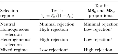
The results of the test in each type of selection regime are summarized in Table 1, which shows that the joint use of both tests allows detecting every selec-tion regime.
DISCUSSION
In this article, we devised and tested a new neutrality test for quantitative traits, which is a multivariate
Figure2.—Accuracy of the tests under neutral divergence. Among- and within-population MS matrices were estimated by MANOVA for 100 rep-licate simulations of neutral evolution (see methods), at 20-generations time intervals (cor-responding to increasingFstin thex-axis). Each of 10 isolated subpopulations of sizeN¼100 hap-loid individuals with five additive traits under-went mutation, drift, and recombination. For each time point and replicate simulation, ˆrst
was estimated according to Equation 11 and the proportionality of MS matrices was tested (Bartlett-adjusted test). (Left) Test i: box plot of the estimated ˆrst. The estimated 95% C.I.’s of ˆrst (bars) correspond to the predicted C.I.’s (dashed lines) under neutrality, and the esti-mated means (solid squares) are in perfect agree-ment with their predicted value [Fst/(1 Fst), solid line] at all levels of population divergence (Fst x-axis). (Right) Test ii: distribution of theP-values (pooled from all time intervals) of the Bartlett-adjusted test onMSmatrices. The distribution does not differ from the expected uniform [0, 1] (type I error andP-value for the one-sided KS test of comparison with the uniform given on the graph).
extension of the classicQst–Fstcomparison. The idea is
to compare the among-population (D) and within-population (G) covariance matrices and to test the neutral pattern ofD¼Fst/(1Fst)G(for haploids, as in
our simulations, and with a factor 2 for diploids). The test is twofold: (i) testing for equality between an estimate of the proportionality coefficient (ˆrst, Equa-tion 11) and its expectaEqua-tion (Fst/(1Fst)) from neutral
markers and (ii) testing for proportionality itself be-tweenDandG. The first test (test i) is very close to the classicQst–Fstcomparisons but in a rigorous multivariate
framework, while test ii is more akin to the approaches proposed in the studies of G matrix evolution (e.g., Schluter1996). Our tests make use of Flury’s (1988)
framework of sample covariance matrix comparisons
(CPC analysis), with a Bartlett correction for small sample sizes proposed by Eriksen(1987), which proves
essential for realistic sampling designs (,20 popula-tions sampled, Figure 1). Note that the software CPC (Phillips and Arnold 1999), although a pioneer in
divulging the CPC framework among evolutionary biol-ogists, does not use the Bartlett adjustment, which could be problematic for at least some data sets in evolutionary studies, with typically relatively small sample sizes. When using the proportionality test in our particular context, the correction will always be necessary, as one of the degrees of freedom is given by the number of popula-tions (rarely exceeding 10).
Our simulations suggest that, with a realistic sampling design (10 populations, 20 families per population, five
Figure3.—Power to detect nonneutral diver-gence: the same as Figure 2 but with individuals undergoing selection in addition to drift, muta-tion, and recombination. In addition to its ex-pected range under neutrality [Equation 5 inverted with r ¼ Fst/(1 Fst), solid dashed lines], the theoretical C.I. of ˆrst predicted from its observed value (Equation 5 inverted withr¼ mean ˆrst) was also reported (shaded dashed lines), to check the robustness of Equation 5 to nonproportionality betweenMSmatrices. (a) Ho-mogeneous selection for the same optimum: ˆrstis significantly lower than the neutral expectation Fst/(1 Fst) (estimated and predicted C.I.’s do not overlap, left) and theP-value distribution of the Bartlett test is significantly different from uni-form [0, 1] (right). However, in a large propor-tion of simulations, proportionality is not rejected, although false (high type II error risk, indicated on the graph). (b) Heterogeneous se-lection for distinct optima in each population: ˆ
rst is significantly higher thanFst/(1Fst) (left) and theP-value distribution is not uniform [0, 1] but again there is a high type II error risk (right). (c) Mixture of both selection regimes with two traits under heterogeneous selection and three traits under homogeneous selection: this time, ˆ
rst is not significantly different from Fst/(1
traits measured), the predicted neutral pattern is exact when only mutation and drift (and potentially migra-tion) affect the trait (Figure 2) and that different forms of selection can efficiently be detected (Figure 3). The efficiency of this neutrality test stems from the fact that two independent tests are used that are complementary in detecting different types of departures from the neutral pattern (Figure 3 and Table 1). We believe the combined tests have more power than the classic mean
Qst–Fstcomparisons for three reasons. First, the
confi-dence intervals of ˆrst-estimates appear to be fairly reduced even with the limited data sets of our simu-lations, and the effect of sampling on these C.I.’s appears to be accurately predicted by the CPC frame-work. This is often not the case with classic meanQst
estimates over several traits, which have notoriously large C.I.’s and for which the correct statistical inference of the C.I. is problematic, both for univariateQst(as in
O’Hara and Merila 2005) and for their mean over
traits (often with the implicit and wrong assumption of independence between traits). Second, the C.I. for ˆrst (Equation 5) is a simple product of ˆrstby a factor that is determined only by the sampling design (nw, nb, p),
which allows making straightforward power analysis before any empirical study (detailed below). Finally and maybe more importantly, averaging over traits that are under opposite selective forces (mixture regime, Figure 3c) can lead to the erroneous acceptation of neutrality in the classicQstapproach. Logically, it is also the case
based on test i, which is akin to theQst–Fstcomparison;
however, test ii efficiently rejects neutrality in this case as the existence of opposite selection forces breaks down the proportionality between G and D. Overall the combined tests i and ii give a fairly powerful and sta-tistically rigorous framework to detect various selection
regimes, including some that are undetected by the classicQstapproach. Below, we discuss the robustness of
our theoretical and statistical results, practical implica-tions for empirical designs, and future developments of this approach to study multivariate evolution in natural populations.
Robustness of the theoretical expectation and the statistical method: Our simulations made precise as-sumptions for the genetic basis of the quantitative traits under study. Some are required for the theoretical prediction (Equation 2) to be valid (additivity and neutrality of the loci, no linkage disequilibrium), and some are not. For instance, as for its univariate version in Whitlock (1999), Equation 2, being derived from
coalescent theory, is independent of the ecological mechanism ofneutralpopulation divergence (migration between demes of arbitrary sizes, isolation by distance, extinction/colonization dynamics, etc.), although we simulated only the simpler case of identical and isolated demes. As an example, this is confirmed in simulations of a finite-island model with migration, provided in supplemental Figure 1. Similarly, heterogeneity among loci for mutational effects, or the number of loci itself, does not influence our results based only on the total mutational variance, summed over loci (Equation 1); this was confirmed by simulations (not shown), for the number of loci. The choice of an alternative mutation model to the house of cards with Gaussian distribution of effects in our simulations should also not influence the results, as long as the mutational covariance between traits remains independent of the current state of the individual (Whitlock1999) and as long as the breeding
value distribution for each trait remains approximately Gaussian. For example, Equation 2 should still be valid in the classic infinite-allele model (Kimuraand Crow
1964), where new mutation effects add up to the current allele effect at each locus, but are still drawn into a distribution that is independent of the current state. Our results should in fact still be valid when mutational covariances change through time, but the netinput of mutational covariance averaged over generations is the same along every branch of the coalescent (i.e., within each subpopulation). Finally, because Equation 2 is based on coalescent theory, wrong identification of the subpopulation units in the field (e.g., if one of the samples includes in fact several biological subunits) should not invalidate the prediction under neutrality. Under selective divergence, however, such erroneous sampling would lead to including part of the among-population divergence in the within-among-population level. This may tend to artificially align GwithDand could favor the neutrality hypothesis, when selection is in fact occurring. In this case, ˆrstshould still be different from its neutral expectation (test i), but this difference may not be significant anymore. Therefore, correct identification of biological subpopulation units is re-commended, as is the case for many methods in TABLE 1
Results of the neutrality tests according to the selection regime
Selection regime
Test i: ˆ
rst¼Fst=ð1FstÞ
Test ii:
MSbandMSw proportional
Neutral Minimal rejection Minimal rejection Homogeneous
selection
High rejection Low rejectiona
Heterogeneous selection
High rejection Low rejectiona
Mixed regime Low rejectiona High rejection
For all divergence scenarios considered in Figures 2 and 3 the outcome of the two neutrality tests in our simulations is summarized. Both tests are accurate under neutrality but in all cases of selection, one of them fails. However, at least one test is accurate so that the joint use of tests i and ii allows detecting all selection regimes.
a
An outcome that does not correspond to the correct situ-ation (in all cases it corresponds to a high type II error risk).
metapopulation studies. Note that molecular markers could be used to this end, with identification of units via Bayesian clustering algorithms (e.g., Pritchard
et al.2000).
Moreover, discrepancies with basic assumptions of the model may not always invalidate its results. Linkage disequilibrium between loci determining the traits is assumed to be negligible in the coalescent approach we used (Whitlock 1999). However, as detailed in (Le
Correand Kremer2003), significant linkage
disequi-librium need not affect theQst¼Fstrelationship (nor its
multivariate equivalent in Equation 2) provided that it affects the between-population and the within-population covariances similarly. There are two possible sources of genetic covariance between traits: linkage disequilib-rium and pleiotropic mutation. In this article, the mecha-nism studied is pleiotropy, but interestingly, when linkage disequilibrium, not pleiotropic mutation, is the source of the genetic covariance between traits, Equation 2 was also obtained by Rogersand Harpending(1983),
although only for diallelic and nonpleiotropic loci and in an island model. However, we can expect that when neutral divergence occurs with an initial negative linkage disequilibrium buildup by past selection (Bulmer effect), the value of r may tend to fall below its neutral ex-pectation (which assumes linkage equilibrium), as pre-dicted by LeCorreand Kremer(2003) for univariateQst
measures. This effect should be even stronger with asexual populations. Finally, as shown in methods, in
the case of species with some level of inbreeding, the test can still be performed but a correction must be applied by changing the expected ratio in Equation 2 to 2Fst/
((1 Fst)(1 1 Fis)), where Fis is the inbreeding
co-efficient, also estimated from the neutral marker data. Regarding Fst estimation, the relevant Fst value in
Equation 2 should be that of the loci encoding the quantitative traits (QTL) under study and may differ from that empirically measured on neutral markers. However, as discussed in Whitlock (1999), when the
influence of mutation onFstis weak relative to that of
demography and the genetic system (strong drift and/or migration relative to the mutation rate for both markers and QTL), Fst is mainly determined by demography,
common to both markers and QTL, so that the neutral pattern can be tested withFstfrom neutral markers.
We can see two key assumptions to which the results should be sensitive: normality of the breeding values and additivity across loci encoding the traits. The method should be fairly strongly dependent on the normality assumption, as is the case for both the CPC analysis framework (Flury1988) and the parametricQst
estimation methods (O’Haraand Merila2005).
Con-sequently, proper transformation of the phenotypic data to conform to the Gaussian assumption is recom-mended before analyzing the empirical data. We did not study the effect of nonnormality on the tests presented here, but one prediction can be made. When traits are
non-Gaussian, the deviance of all models in the CPC analysis should be lower (as the Wishart distribution does not give a good fit to the sample covariance esti-mates), whereas the number of parameters for each model will remain unchanged. Therefore, (i) the propor-tionality test may reject the neutral pattern even when it is in fact correct (type I error), and (ii) the estimate ofr and its C.I. may be incorrect. The first point should artificially favor selective interpretations against neutral ones. The second one may induce any unwanted effect (type I or II error) and we did not study this impact here. Our simulations (Figure 3) revealed that the C.I. forrwas fairly correctly predicted by Equation 5, even under nonneutral conditions for which the proportionality as-sumption was violated. Consequently, we may suspect that test i based on the comparison ofrwith 2Fst/(1Fst)
should also be more robust to nonnormality than test ii. However, again, proper standardization of the data to approach normality is a general recommendation in many multivariate analyses, and this method is no exception.
Nonadditivity of the quantitative traits, even neutral, is an acknowledged source of bias in Qst–Fst
com-parisons, leading, in most cases, to a downward bias ofQstrelative toFst. Both additive-by-additive variance
(Whitlock 1999) and dominance variance (Goudet
and Buchi2006) affecting a neutral trait are expected
to lowerQstrelative toFst, which in our case would lead
to a value ofr, 2Fst/(1Fst). Note that this effect is
expected in many but not all cases when there is only dominance variance (discussed in Goudetand Martin
2007; Lopez-Fanjul et al. 2007). Together with the
probable negative bias induced by negative linkage disequilibria due to past selection, these results suggest that a pattern ofr,2Fst/(1Fst) should be interpreted
with some caution, as previously outlined (Whitlock
1999; Goudetand Buchi2006) for the univariateQst–
Fstcomparison. Such a pattern (if weak, at least) may
reflect nonadditivity or linkage disequilibria affecting otherwise approximately neutral traits. On the contrary, the opposite pattern r . 2Fst/(1 Fst) can be taken
with greater reliability as evidence of heterogeneous selection.
Finally, in some studies, the phenotypic covariance matrixP is used as a proxy for the genetic covariance matrixG, because it is easier to estimate. If our tests are applied to phenotypic distributions instead of breed-ing value distributions, environmental variance might influence the result. LetEbe the environmental covari-ance matrix within subpopulations. Then the within-population phenotypic covariance isPw¼G1Ewhile
the between-population phenotypic covariance isPb¼
D1E/nb(nbis the number of populations), so that the
environmental variance increases Pw more than Pb
and creates a bias. In the neutral case whereD¼Fst/
(1 Fst)G, the relationship on phenotypic covariances
will be Pb , Fst/(1 Fst)Pw, with nonproportionality
stabilizing selection. The impact of this bias is larger with smaller Fst and larger environmental varianceE.
Overall it is therefore advisable to apply the test on breeding values, and when applied on phenotypic values and rejecting proportionality with a patternr, 2Fst/(1 Fst), the results will again have to be
inter-preted with caution, as with nonadditivity (above). We did not simulate all departures from our model assumptions. However, on the basis of the above the-oretical arguments and our simulations, we believe that the test presented in this article is fairly robust to several genetic and ecological details underlying quantitative variation in a metapopulation. Yet, we note that some departures from the basic assumptions of the model may lead to erroneous conclusions. In this regard, the test on ˆrst-values (test i) is probably more robust than the proportionality test (test ii).
Best experimental design and method to detect selection: The analytic expression of the C.I. for r (Equation 5) gives a straightforward basis for optimization of any empirical sampling design. Two conclusions can be drawn from this equation and from our study in general. First, the number of traits (p) and the effect of sampling [harmonic mean of sampling sizes between and within populations (1/nw11/nb)] act
multiplica-tively to reduce the sample variance of ˆrst, so that it is not necessary to pool numerous traits together if the sampling design is large enough. This is important in the perspective of being able to distinguish between different types of traits: indeed, by choosing a biologi-cally coherent set of traits (e.g., morphological, life history, etc.), which may be rather small, the results can be interpreted with more relevance. Second, the sam-pling effort should be balanced as much as possible between the among-population and the within-popula-tion levels, as the sampling variance decreases with the harmonic mean of relative sample sizes (1/nw11/nb).
Furthermore, the x2-distribution of the log-likelihood
ratio (Equation 7) under proportionality, even with the Bartlett correction of Eriksen(1987), is an asymptotic
result that is more accurate when bothnband nw are
large (in our simulations, at least 10, Figure 1). Overall, this means that sampling of many populations is advis-able to get a more accurate measure of ˆrst(test i) and a more reliable proportionality test (test ii). On the contrary, the number of families per population may be rather small if many populations are sampled: the within-population degree of freedom in the MANOVA (nw) will still remain large. Finally, the required number
of populations to be sampled increases with the number of traits studied for the proportionality test (at leastnb.
p), which again argues in favor of avoiding the study of too many traits together. Overall, to detect selection, we recommend that sampling efforts in studies of meta-populations be oriented to considering more popula-tions (e.g., .10–20), even at the cost of a reduced number of families per population or of a reduced
number of traits measured. Again, power analysis can be carried out very easily as the sample variance ofrhas a simple close form (Equation 5), a main advantages of this test compared to several classic methods of Qst
estimation.
Because it is directly based on the estimation of variance components from the data set by MANOVA, the method can be extended to hierarchical designs (e.g., populations within habitats, etc.), using the correspond-ing mean square matrices (MS) and degrees of free-dom. However, the power and the accuracy of the tests will be reduced at higher levels of the hierarchy for which the degrees of freedom are very small (often two habitats so that d.f.¼1). This makes the proportionality test (test ii) irrelevant as it requires d.f.. pfor allMS matrices. However, test i could still be applied as the estimate and C.I. of ˆrst seems valid even for very low degrees of freedom (Figure 1a). Nevertheless, ˆrstat the habitat level will likely have a very large C.I. in this case, which would also greatly reduce the power of the test. Improvements of the test to gain power in the study of a small number of groups will be necessary in the future to provide powerful tests based on quantitative genetic data from,e.g., two distinct habitats. Meanwhile, it may be best to study larger sets of habitat types (e.g., using several thresholds along a gradient).
Further issues: The main problem common to all multivariate Qst analyses (means over traits or our
method) is that different traits are pooled and the net effect of evolutionary forces on the whole trait set is the only information available. This problem is partly over-come by our approach, which can detect when distinct subsets of traits are under qualitatively different selection regimes. However, it remains a ‘‘pooled-traits’’ approach for which individual traits information is lost. The alternative of using single-trait Qst is obviously worse,
as such, because in most cases the C.I. for eachQstis of
the order of [0, 1] and is sometimes not easy to compute (O’Haraand Merila 2005), so that a test against the
value of Fst has no power and may be inaccurate. To
allow the proper biological interpretation of the type of multitrait analysis presented here, it is therefore best to consider sets of biologically coherent traits for which similar evolutionary forces are expected to act. Such
an a priori interpretation is always difficult to state,
but because the method can detect mixed selection regimes, it may be possible to conduct exploratory studies and find the set of biologically coherent traits to be analyzed.
In molecular evolution, the same problem applies: neutrality tests have been designed that use compar-isons of diversity between populations (divergence between species) and within populations (polymor-phism within species) such as the McDonald–Kreitman test (McDonaldand Kreitman1991), in a way akin to
theQst–Fstmethod. An inherent limit to these methods
is that information from different nucleotide sites/