Transactions of the 17th International Conference on Structural Mechanics in Reactor Technology (SMiRT 17) Prague, Czech Republic, August 17 –22, 2003
Paper # C04-4
Presentation of a New Methodology of Chained Computations using
Instationary 3D Approaches for the Determination of Thermal Fatigue in a
T-Junction of a PWR Nuclear Plant
Sofiane Benhamadouche1), Marc Sakiz1), Christophe Péniguel1), Jean-Michel Stéphan2)
1) EDF R&D, MFTT Dpt, 6 quai Watier, 78401 Chatou, FRANCE 2) EDF R&D, MMC Dpt, 77818, Moret-sur-Loing, FRANCE
ABSTRACT
Thermal fatigue of the coolant system of PWR plants is a major issue for nuclear safety. The problem is especially accute in mixing zones, like T-junctions, where a large difference of water temperature between the two entry branches and the high level of turbulence can lead to large temperature fluctuations at the wall. Until now, studies on this matter have been tackled at EDF using steady methods. The purpose of this paper is to present a new methodology of chained computations, that allows to take into account the unsteady and 3D effects of the problem, and apply it to the Residual Heat Removal (RHR) system. A development version of EDF finite volume CFD tool Code_Saturne is used to compute the fluid flow with a L.E.S. model, which gives access to the instantaneous temperature fluctuations.
Code_Saturne is coupled to the finite element thermal code Syrthes, which propagates the temperature fluctuations into the wall thickness. Then, the instantaneous temperature field inside the wall is transfered to EDF thermomechanic tool
Code_Aster, to perform mechanical computations that yield the instantaneous mechanical stresses seen by the T-junction and the following elbow. The results of this first study are promising, although this method is still largely under development and validation.
KEYWORDS: nuclear power plant, coolant system, RHR, thermal fatigue, thermohydraulics, numerical simulation, Large Eddy Simulation, CFD, turbulence, Code_Saturne, Syrthes, code coupling,
INTRODUCTION
Thermal fatigue of the coolant systems of PWR plants is a major issue for nuclear safety. The problem is especially accute in mixing zones, like T-junctions, where a large difference of water temperature between the two entry branches and the high level of turbulence can lead to large temperature fluctuations at the wall. Civaux N4 class reactor was shut down in may 1998 following a leak of primary coolant from a pipe in the Residual Heat Removal (RHR) system. Cracks have been discovered in the elbow following the T-junction, that were clearly the result of thermal fatigue. Since then, the RHR pipeworks have been redesigned at all four EDF's N4 units.
The aim of the present study is to get a better understanding of the thermal loads seen by the structure in such situation. In order to deal properly with such problems, instantaneous thermohydraulic phenomena, thermal coupling between the fluid and the solid, as well as the thermal conduction inside the wall have to be accounted for. These aspects are described in detail in the present paper. Eventually, the 3D instantaneous solid temperature fields obtained are used to compute the resulting mechanical stresses (as presented in [1]). But this last aspect is beyond the scope of this paper.
NUMERICAL APPROACH OF INTANTANEOUS THERMOHYDRAULIC PHENOMENA
To improve the design of some components or explain why a failure has occured, engineers try to gain some understanding of the phenomena taking place or what components should be modified to meet safety requirements. Experimental approaches have been extensively used but they may become quite costly when dealing with high temperature, pressure or potentially dangerous environments (as it is the case in nuclear industry). Moreover, on-site experimental approaches often lack the flexibility needed when a sensitivity study is desired.
limited to extremely low Reynolds numbers (a few thousands at most), and is therefore incompatible with industrial configurations.
Large Eddy Simulation (L.E.S.) can be seen as an intermediate technique between D.N.S. and R.A.N.S. The contribution of large energy carrying structure is computed exactly while the smaller scales of turbulence are modelled. Thus L.E.S. still provides 3D time dependent solutions and can be used at much higher Reynolds Numbers.
The CFD Tool Code_Saturne
The EDF finite volume CFD code, Code_Saturne, is used to solve Navier-Stokes equations on unstructured meshes. The flow is assumed incompressible and Newtonian and the density is only function of temperature. Using L.E.S., the filtered Navier-Stokes equations can be written (the filtering operator is omitted used for clarity sake):
0 x U t j j = ∂ ∂ρ + ∂ ∂ρ (1) i 0 j j e i i j j i e j i j i j
i ( )g
x U x 3 2 x U x U x x * p x U U t
U + ρ−ρ
∂ ∂ µ ∂ ∂ − ∂ ∂ + ∂ ∂ µ ∂ ∂ + ∂ ∂ − = ∂ ∂ ρ + ∂ ∂ ρ (2)
In these equations, Ui are the filtered components of the velocity, p* stands for the pressure (minus the reference
hydrostatic pressure), µe represents µ+µt where µ and µt are respectively the molecular and turbulent viscosities. It
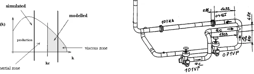
should be noted that in k-ε approaches, the turbulent viscosity models the turbulent effects on the whole energy spectrum, whereas in L.E.S. it represents only the small scales structures (high frequencies), as shown in figure 1 for the idealistic spectrum of homogeneous isotropic turbulence. The turbulent viscosity µt relies on the Smagorinsky
model:
( )
ij ij 2 st = C∆ 2SS
µ (3)
where Sij is the filtered strain tensor and ∆ the lenght scale of the filter. In the framework of a finite volume
approach, one may consider ∆=2Ω1/3, where Ω is the volume of the cell. Smagorinsky constant C
s is set to 0.065
(common value for channel flows). Regarding, the near-wall modelling, L.E.S. relies on a power low wall function. More details on LES in Code_Saturne can be found in [2], [3] and [4].
Before taking on the study presented here, Code_Saturne and its L.E.S. development version have been tested on a large number of academic and industrial validation cases (homogeneous turbulence, channel flows, tube bundles, T-junction, coaxial jet, …).
Numerical Technique Used for Solving the Fluid Equations
In the collocated finite volume approach used in Code_Saturne, all variables are located at the centres of gravity of the cells (which may take any shape). The momentum equations are solved by considering an explicit mass flux (the three components of the velocity are thus uncoupled). Velocity and pressure coupling is insured by a prediction/correction method with a SIMPLEC algorithm [5]. The Poisson equation is solved with a conjugate gradient method. The collocated discretization requires a Rhie and Chow [6] interpolation in the correction step to avoid oscillatory solutions. This interpolation has been used in the present application, although it doesn't seem essential for unstructured meshes. For L.E.S. calculations, second order schemes are used in space (fully centred scheme for the velocity components, centered scheme with slope test for the temperature) and time (Crank-Nicolson with linearized convection). A second order Adams-Bashforth method is used for the part of the diffusion involving the transposed velocity gradient, to keep the velocity components uncoupled.
The Solid Code Syrthes
The solid code Syrthes relies on a finite element technique to solve the general heat equation (4) where all properties can be time, space or temperature dependent.
v j s j p x T k x t T
C +Φ
∂ ∂ ∂ ∂ = ∂ ∂ ρ (4)
T is the temperature, t the time, Φv a volumic source or sink, ρ and Cp, respectively the density and the specific
been retained (6 nodes triangles in 2D, 10 nodes tetrahedra in 3D). More details on the possibilities of the finite element code Syrthes can be found in [7] and [8]. Like the fluid code, Syrthes has been checked thoroughly against experimental and analytical test cases proving that it provides very accurate solutions in problems similar to the present one.
Heat Transfer at the Fluid/Solid Interface
At the interface, every time step, the thermal coupling is performed. This coupling relies on an iterative procedure. Let Ts be the temperature of an internal solid node, Tw the temperature at a node which belongs to the
interface, and Tf the temperature of a fluid point (located generally in the log layer). At time t(n), the CFD tool
Code_Saturne provides after calculation:
h(n): the local heat exhange coefficient at time t(n)
Tf(n): the local inside fluid temperature at time t(n)
using these data, the flux to be applied to the solid is :
(
(n))
f ) 1 n ( w ) n ( ) 1 n (
s =h T −T
ϕ + + (5)
Then, using this flux or the exchange conditions h(n) and T
f(n), Syrthes can solve the heat conduction equation
inside the solid. This gives an updated temperature over all the solid region. These new values Ts(n+1), are also updated
on the boundary. Therefore Tw(n+1) is also known and the iterative procedure may keep going on.
SIMULATED CONFIGURATION General Configuration
The global geometry of the RHR circuit is presented in figure 2. Due to the difficulty and the cost of a CFD approach using Large Eddy Simulation, only the small portion surrounding the location where cracks have occured has been simulated as shown in figure 3. Moreover, in the present study, small bumps corresponding to the weld seams, have been omitted.
Figure 1: Simulated and modelled parts Figure 2: Sketch of the RHR at Civaux 1 of the energy spectrum in L.E.S. (former configuration)
In this specific study, the horizontal hot branch and the vertical cold branch are set respectively at a temperature of 168°C and 41°C. The total flow rate is set to be 1000 m3/h and the velocity ratio between the cold flow branch and
the total flow rate is 20%.
Meshes
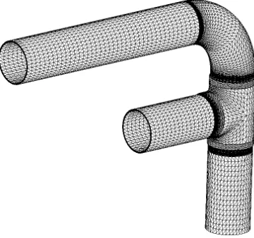
In order to solve the former equations numerically, the geometry has to be dicretized. Here the mesh generators GiBi and Ideas have been used. Figure 4 presents the fluid mesh, it contains 401 472 cells. Likewise, the solid mesh is presented in figure 5. It contains 958 975 nodes and 688 320 tetraedra.
Figure 3: Detail of the simulated T-junction Figure 4: Mesh of the fluid domain and elbow (former configuration)
Figure 5: Mesh of the solid domain Figure 6: Detail of the T-junction in the solid mesh
COMPUTATIONAL RESULTS
This calculation gives access to unsteady results on the entire solid and fluid domains. 10 seconds of physical time have been simulated, which corresponds to an already very large computational effort (around 1000 hours of CPU on a Fujitsu VPP5000 vector machine). Results are mainly presented on four sections and the symmetry plane for which experimental measurements are available on site. These sections are pointed out in figure 7. All thermal results are presented in non-dimensional variables; let Tcold and Thot be the cold and hot temperatures in the branches, the
non-dimensional temperature and RMS temperature are calculated as:
cold hot
cold dim
a
T T
T T T
− −
= and
cold hot dim Ta
T T
T T
− ′ ′ =
σ (both variables varie between 0 and 1) (6)
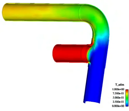
Figure 7: Sections with experimental probes Figure 8: Instantaneous velocity field in the symmetry plane (t=4 s), coloured by the temperature
Figure 9: Instantaneous velocity field in Figure 10: Instantaneous fluid temperature field 4 sections (t=4 s), coloured by the temperature in the symmetry plane (t=4 s)
Temperature Evolution at the Fluid/Solid Interface
The focus is put on points located at the fluid/solid interface, corresponding to experimetal probes on the nuclear plant circuit (of course, experimental probes can only be placed on the outside part of the pipe).
Figures 14 and 15 point out, on sections C1 and PF, the strong attenuation of the temperature signal of the wall compared to the very fluctuating temperature signal of the fluid (upper part of the elbow) in the near wall region. This attenuation is due to the thermal inertia of the wall and is strongly dependent on the frequency of the fluctuations. This dependence is naturally reproduced by our unsteady simulation, whereas it is totally unreachable through averaged R.A.N.S. based approaches. Also, these figures indicate that a strong mixing takes place downstream of the T-junction, the fluid temperature fluctuations being much smaller in section PF than in section C1.
One can also underline the change in the temperature signal at the fluid/solid interface by presenting in figure 16 a temperature histogram of a point located on the upper elbow (section C1).
Temperature Evolution within the Wall
Figure 11: Mean fluid temperature field in the Figure 12: Fluid RMS temperature field in the
symmetry plane symmetry plane
Figure 13: Instantaneous solid temperature field Figure 14: Fluid and solid temperature evolution at (half geometry) at t=4 s fluid/solid interface (upper elbow section C1)
COMPARISON WITH ON-SITE EXPERIMENTAL DATA
The results of our simulation will now be compared to experimental data taken from on-site measurements. It should yet be underlined that on-site recording of the temperature inside the pipe is not possible. Hence, the measurements of temperature in the pipe at the fluid/solid interface are in fact obtained indirectly from a deformation probe on the outside part of the wall. Also, the characteristics of the on-site configuration differ slightly from the simulation (22.2% on site velocity ratio instead of 20% and 1025 m3/h on site flow instead of 1000 m3/h). Moreover the
locations of the probes differ slightly, since it is impossible on site to install probes on the symmetry plane.
Instantaneous Temperature Evolution
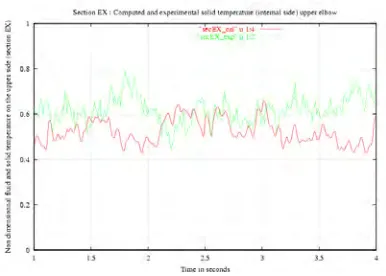
Figures 18 to 21 show temperature profiles (over 3 seconds of physical time) taken from experimental data and from the simulation. Probes are located on the upper elbow, at different sections (cf. figure 7). It appears that:
- turbulent fluctuating phenomena seems to be well captured. - fluctuations amplitude seems to be of the right order.
- experimental and simulated signals seem to have similar frequencies (see also fig. 22).
Figure 17: RMS temperature through the wall Figure 18: Internal temperature on the upper (upper elbow, section C1) elbow (section C1)
Figure 19: Internal temperature on the upper elbow Figure 20: Internal temperature on the upper elbow
(section C2) (section EX)
Mean and RMS Temperature
A more classical way to compare simulation and experimental data is to compare mean and RMS temperature. Table 1 gives these two quantities at the fluid/solid interface on the upper part of the elbow. Considering the differences mentionned above, one may argue that experimental and computed data show reasonnable agreement.
Spectral Density Power
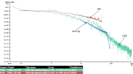
Since the approach gives access to the instantaneous temperature evolution, one may also apply usual spectral analysis. Figure 22 presents the Spectral Density Power obtained from experimental signals (on site and a mock-up) and from the L.E.S. approach for the probe located in section EX (upper elbow, fluid/solid interface).
spectral technique. Nevertheless, the different profiles seem in good agreement, and none of them shows any specific frequency peak.
Figure 21: Internal temperature on the upper elbow Figure 22: Experimental and L.E.S. temperature SDP (section P1)
section Tadim (exp.) Tadim (comp.) σTadim (exp.) σTadim (comp.)
C1 0.11 0.20 0.078 0.050
C2 0.72 0.60 0.088 0.055
EX 0.61 0.52 0.081 0.053
P1 0.82 0.67 0.082 0.048
Table 1: Experimental and computation comparison
CONCLUSION AND PERSPECTIVES
This paper presents a numerical approach able to address thermal fatigue problems occuring in pipeworks. A Large Eddy Simulation turbulent model implemented in EDF's CFD tool Code_Saturne yields instantaneous velocity and temperature fields. The thermal coupling with the finite element thermal code Syrthes allows to have access to the instantaneous thermal field inside the wall. These solid thermal fields are then exploited with a mechanical tool to obtain thermally induced stresses (see paper [1] for the methodology).
The L.E.S. approach seems very promising when compared to experimental data, to get a better understanding and knowledge of the instantaneous thermal loads seen by pipeworks, although still very costly in terms of CPU and computing memory. Further studies are planned at EDF to improve CPU aspects and confirm on other industrial configurations the ability and the high interest of the thermally coupled approach presented in this paper. Special efforts are likely to be devoted to investigating the influence of the inlet unsteady conditions and the near wall modelling in L.E.S.
REFERENCES
1. Stéphan J.M., Curtit F., Vindeirinho C., Taheri S., Akamatsu M., Péniguel C., « Evaluation of the Risk of Damages in Mixing Zones: EDF R&D Program », Proceeding ASME-PVP, Vancouver, 2002.
2. Benhamadouche S., Implantation de la L.E.S. dans une version de développement de Code_Saturne, Internal EDF R&D report HI-83/01/025.
3. Benhamadouche S., Laurence D., « L.E.S., Coarse L.E.S., and Transient RANS Comparisons on the Flow across a Tube Bundle », 5th Int. Symp. on Engineering Turbulence Modelling and Measurments, Mallorca, Spain 16-18 September 2002, W Rodi and N. Fueyo Edts, Elsevier.
4. Benhamadouche S., Mahesh K., Constantinescu G., « Collocated Finite Volume Schemes for L.E.S. on Unstructured Meshes », CTR, Proceeding of the 2002 Summer Program Stanford.
5. Ferziger J.H., Períc M., Computationnal Methods for Fluid Dynamics, Springer, second edition, 1999.
6. Rhie C.M., Chow W.L., « A Numerical Study of a Turbulent Flow past an Isolated Airfoil with Training Edge Separation », AIAA paper, 82-0998.
7. Péniguel C., Rupp I., « Coupling Heat Conduction and Radiation in Complex 2D and 3D Geometries », Proceeding Numerical Methods in Thermal Problems, Swansea, 1997.