On the complexity of computing determinants

ON THE COMPLEXITY OF COMPUTING

DETERMINANTS

Erich Kaltofen and Gilles Villard

To B. David Saunders

on the occasion of his 60th birthday

Abstract. We present new baby steps/giant steps algorithms of asymptotically fast running time for dense matrix problems. Our al-gorithms compute the determinant, characteristic polynomial, Frobe-nius normal form and Smith normal form of a dense n_×n _matrix A with integer entries in (n3.2_logkA_k)1+o(1) _{and (}n2.697263_logkA_k)1+o(1) bit operations; here kA_{k denotes the largest entry in absolute value} and the exponent adjustment by “+o_{(1)” captures additional factors} C_1(logn₎C2_(loglogkAk)C3 _{for positive real constants C}

1, C2, C3. The

bit complexity (n3.2_logkA_k)1+o(1) _{results from using the classical cubic} matrix multiplication algorithm. Our algorithms are randomized, and we can certify that the output is the determinant of A _{in a Las Vegas} fashion. The second category of problems deals with the setting where the matrix A _{has elements from an abstract commutative ring, that is,} when no divisions in the domain of entries are possible. We present algorithms that deterministically compute the determinant, character-istic polynomial and adjoint of A _with n3.2+o(1) _and O₍n2.697263_{) ring} additions, subtractions and multiplications.

Keywords. integer matrix, matrix determinant, characteristic poly-nomial, Smith normal form, bit complexity, division-free complexity, randomized algorithm, multivariable control theory, realization, matrix sequence, block Wiedemann algorithm, block Lanczos algorithm

Subject classification. 68W30 symbolic computation and algebraic computation, 15A35 matrices of integers

1. Introduction

lengths of the integers involved in the computation and the answer affect the running time of the used algorithms. A classical methodology is to compute the results via Chinese remaindering. Then the standard analysis yields a number of fixed radix, i.e. bit operations for a given problem that is essentially (within polylogarithmic factors) bounded by the number of field operations for the problem times the maximal scalar length in the output. The algorithms at times use randomization, because not all modular images may be usable. For the determinant of an n ×n integer matrix A one thus gets a running time of (n4_logkAk)1+o(1) _{bit operations (von zur Gathen & Gerhard 1999,}

Chapter 5.5), because the determinant can have at most (nlogkAk)1+o(1)_digits;

by kAk we denote the largest entry in absolute value. Here and throughout this paper the exponent adjustment by “+o(1)” captures additional factors C1(logn)C2(loglogkAk)C3 for positive real constantsC1,C2,C3 (“soft-O”). Via

an algorithm that can multiply twon×nmatrices inO(nω_{) scalar operations the}

time is reduced to (nω+1_logkAk)1+o(1)_{. We can setω = 2.375477 (Coppersmith}

& Winograd 1990).

First, it was recognized that for the problem of computing the exact rational solution of a linear system the process of Hensel lifting can accelerate the bit complexity beyond the Chinese remainder approach (Dixon 1982), namely to cubic inn without using fast matrix multiplication algorithms. For the deter-minant of an n×n integer matrixA, an algorithm with (n3.5_logkAk1.5₎1+o(1)

bit operations is given by Eberlyet al. (2000).1 _{Their algorithm computes the}

Smith normal form via the binary search technique of Villard (2000). Our algorithms combine three ideas.

i) The first is an algorithm by Wiedemann (1986) for computing the determi-nant of a sparse matrix over a finite field. Wiedemann finds the minimum polynomial for the matrix as a linear recurrence on a corresponding Krylov sequence. By preconditioning the input matrix, that minimum polynomial is the characteristic polynomial and the determinants of the original and preconditioned matrix have a direct relation.

ii) The second is by Kaltofen (1992) where Wiedemann’s approach is applied to dense matrices whose entries are polynomials over a field. Kaltofen achieves speedup by employing Shank’s baby steps/giant steps technique for the computation of the linearly recurrent scalars (cf. (Paterson & Stockmeyer 1973)). For integer matrices the resulting randomized algorithm is of the

1

Eberly et al. (2000) give an exponent for logkA_{k of 2}._{5, but the improvement to 1}.₅

Las Vegas kind—always correct, probably fast—and has worst case bit com-plexity (n3.5_logkAk)1+o(1) _{and again can be speeded with sub-cubic time}

matrix multiplication (Kaltofen & Villard 2001). A detailed description of this algorithm, with an early termination strategy in case the determi-nant is small (cf. (Br¨onnimann et al. 1999; Emiris 1998)), is presented by Kaltofen (2002).

iii) By considering a bilinear map using two blocks of vectors rather than a single pair of vectors, Wiedemann’s algorithm can be accelerated (Copper-smith 1994; Kaltofen 1995; Villard 1997a,b). Blocking can be applied to our algorithms for dense matrices and further reduces the bit complexity.

The above ingredients yield a randomized algorithm of the Las Vegas kind for computing the determinant of an n × n integral matrix A in (n3+1/3_×

logkAk)1+o(1) _{expected bit operations, that with a standard cubic matrix}

mul-tiplication algorithm. If we employ fast FFT-based Pad´e approximation algo-rithms for matrix polynomials, for example the so-called half-GCD algorithm (von zur Gathen & Gerhard 1999) and fast matrix multiplication algorithms, we can further lower the expected number of bit operations. Under the as-sumption that twon×n matrices can be multiplied in O(nω_{) operations in the}

field of entries, and ann×n matrix by an n×nζ _{matrix in n}2+o(1) _operations,

we obtain an expected bit complexity for the determinant of

(1.1) (nηlogkAk)1+o(1) with η =ω+ 1−ζ

ω2_{−(2 +ζ)ω+ 2}.

The best known values ω = 2.375477 (Coppersmith & Winograd 1990) and ζ = 0.2946289 (Coppersmith 1997) yield η = 2.697263. For ω = 3 and ζ = 0 we have η= 3 + 1/5 as given in the abstract above.

Our techniques can be further combined with the ideas by Giesbrecht (2001) to produce a randomized algorithm for computing the integer Smith normal form of an integer matrix. The method becomes Monte Carlo—always fast and probably correct—and has the same bit complexity (1.1). In addition, we can compute the characteristic polynomial of an integer matrix by Hensel lifting (Storjohann 2000b). Again the method is Monte Carlo and has bit complexity (1.1). Both results utilize the fast determinant algorithm for matrix polynomials (Storjohann 2002, 2003).

(see caseiii above) can be applied to our original 1992 division-free algorithm, and we obtain a deterministic algorithm that computes the determinant and characteristic polynomial of a matrix over a commutative ring in nη+o(1) _ring

additions, subtractions and divisions, where η is given by (1.1). The exponent η = 2.697263 seems to be the best that is known today for the division-free determinant problem. By the technique of Baur and Strassen (1983) we obtain the adjoint of a matrix in the same division-free complexity.

Kaltofen and Villard (2004) have identified other algorithms for computing the determinant of an integer matrix. Those algorithms often perform at cubic bit complexity on what we call propitious inputs, but they have a worst case bit complexity that is higher than our methods. One such method is Clarkson’s algorithm (Br¨onnimann & Yvinec 2000; Clarkson 1992), where the number of mantissa bits in the intermediate floating point scalars that are necessary for obtaining a correct sign depends on the orthogonal defect of the matrix. If the matrix has a large first invariant factor, Chinese remaindering can be employed in connection with computing the solution of a random linear system via Hensel lifting (Abbott et al. 1999; Pan 1988).

Notation: BySm×n _{we denote the set ofm×n matrices with entries in the}

setS. The set Zare the integers. For A∈Zn×n we denote by kAk the matrix height (Kaltofen & May 2003, Lemma 2):

kAk=kAk∞,1 = max

x6=0 kAxk∞/kxk1 = max1≤i,j≤n|ai,j|.

Hence the maximal bit length of all entries in A and their signs is, depending on the exact representation, at least 2 +blog₂max{1,kAk}c. In order to avoid zero factors or undefined logarithms, we shall simply definekAk>1 whenever it is necessary.

when cubic matrix multiplication algorithms are employed (Theorem 4.2). Sec-tion 5 presents the division-free determinant algorithm. SecSec-tion 6 contains the analysis for versions of our algorithms when fast matrix multiplication is intro-duced. The asymptotically best results are derived there. Section 7 presents the algorithms for the Smith normal form and the characteristic polynomial of an integer matrix. We give concluding thoughts in Section 8.

2. Generating polynomials of matrix sequences

Coppersmith (1994) first has introduced blocking to the Wiedemann method. In our description we also take into account the interpretation by Villard (1997a; 1997b), where the relevant literature from linear control theory is cited. Our algorithms rely on the notion of minimum linear generating polynomials (gen-erators) of matrix sequences. This notion is introduced below in Section 2.1. We also see how generators are related to block Hankel matrices and recall some basic facts concerning their computation. In Section 2.2 we then study determinants and Smith normal forms of generators and see how they will be used for solving our initial problem. All the results are given over an arbitrary commutative fieldK.

2.1. Generators and block Hankel matrices. For the “block” vectors X ∈Kn×l and Y ∈Kn×m consider the sequence of l×m matrices

(2.1) B[0] _=XTr

Y, B[1] _=XTr

AY, B[2] _=XTr

A2_{Y, . . . , B}[i] _=XTr

Ai_{Y, . . .}

As in the unblocked Wiedemann method, we seek linear generating polyno-mials. A vector polynomial Pd_i=0c[i]_λi_{, where c}[i] _{∈ K}m_{, is said to linearly}

generate the sequence (2.1) from the right if

(2.2) ∀j ≥0 :

d X

i=0

B[j+i]c[i]=

d X

i=0

XTr

Ai+jY c[i]= 0l.

For the minimum polynomial ofA, fA_{(λ), and for the µ-th unit vector in K}m_, e[µ]_{, f}A_(λ)e[µ] _{∈ K[λ]}m _{is such a generator because it already generates the}

Krylov sequence{Ai_Y[µ]_}

i≥0, where Y[µ] is theµ-th column of Y. We can now

consider the set of all such right vector generators. This set forms a K[λ ]-submodule of the K[λ]-module K[λ]m _{and contains m linearly independent}

(over the field of rational functionsK(λ)) elements, namely allfA_(λ)e[µ]_.

of the matrix formed by those basis vector polynomials as columns is minimal. The matrices corresponding to all integral bases clearly are right equivalent with respect to multiplication from the right by any unimodular matrix inK[λ]m×m_,

whose determinant is by definition of unimodularity a non-zero element inK. Thus we can pick a matrix canonical form for this right equivalence, say the Popov form (Popov 1970) (see also Kailath 1980, §6.7.2) to get the following definition.

Definition 2.3. The unique matrix generating polynomial for (2.1) in Popov form, denoted by F_XA,Y ∈ K[λ]m×m_{, is called the minimum matrix generating}

polynomial (generator).

As we will show below, deg(detF_XA,Y) ≤ n. The computation of the min-imum matrix generating polynomial from the matrix sequence (2.1) can be accomplished by several interrelated approaches. One is a sophisticated gen-eralization of the Berlekamp/Massey algorithm (Coppersmith 1994; Dickinson

et al. 1974; Rissanen 1972). Another generalizes the theory of Pad´e approx-imation (Beckermann & Labahn 1994; Forney, Jr. 1975; Giorgi et al. 2003; Van Barel & Bultheel 1992). The interpretation of the Berlekamp/Massey al-gorithm as a specialization of the extended Euclidean alal-gorithm (Dornstetter 1987; Sugiyama et al. 1975) can be carried over to matrix polynomials (Cop-persmith 1994; Thom´e 2002) (see also Section 3 below). All approaches solve the classical Levinson-Durbin problem, which for matrix sequences becomes a block Toeplitz linear system (Kaltofen 1995). The relation to Toeplitz/Hankel matrices turns out to be a useful device for establishing certain properties.

For a degreedand a lengthewe consider thel·ebym·(d+ 1) block Hankel matrix

(2.4) Hke,d+1(A, X, Y) =

     

B[0] _B[1] _{. . . B}[d−1] _B[d]

B[1] B[2] _B[d] _B[d+1]

... . .. ... ... B[e−1] . . . B[d+e−1]

     

For any vector generator Pd_i=0c[i]_λi _∈Km_{[λ] we must have}

Hke,d+1·

  

c[0]

... c[d]

 

By considering the rank of (2.4) we can infer the reverse. If

(2.5) Hkn,d+1·

  

c[0]

... c[d]

  = 0

then Pd_i=0c[i]_λi _{is a vector generator of (2.1). The claim follows from the fact}

that rank Hkn,d+1 = rank Hkn+e0

,d+1 for all e0 > 0. The latter is justified by

observing that any row in the (n +e0_{)th block row of Hk}

n+e0

,d+1 is linearly

dependent on corresponding previous rows via the minimum polynomial fA_,

which has degree deg(fA_)≤n.

We observe that rank(Hke,d) ≤ n for all d > 0, e > 0 by considering the

factorization

Hke,d=       

XTr XTr

A XTr

A2

... XTr

Ae−1

      

·Y AY A2_{Y . . . A}d−1_Y

and noting that either matrix factor has rank at mostn.

Therefore, whend≥deg(F_XA,Y), the module overK[λ] generated from solu-tions to (2.5) is the module of vector generators, with the columns of F_XA,Y(λ) as basis. In this case, if the column degrees of the minimum generator are δ1 ≤ · · · ≤δm, the dimension of the right nullspace of Hke,d+1 in (2.5) over K

is (d−δ1+ 1) +· · ·+ (d−δm+ 1). Hence for d≥degFXA,Y and e≥n we have

rank(Hke,d+1) =δ1+· · ·+δm = deg(detF_XA,Y)≤n, the latter becauseF_XA,Y(λ)

is in Popov from. Since the last block column in Hke,d+1 with d≥ deg(FXA,Y)

is generated by previous block columns, via shifting lower degree columns of F_XA,Y(λ) as necessary by multiplying with powers ofλ, we have

(2.6) rank(Hke,d) = deg(detFXA,Y) for d≥degF A,Y

X and e≥n.

One may now define the minimum emin such that the matrix Hkemin,d for

d = degF_XA,Y has full rank deg(detF_XA,Y). Any algorithm for computing the minimum generator requires the first deg(F_XA,Y) + emin elements of the

We give an example over Q (Turner 2002). Let A=    

0 1 0 0 0 0 1 0 0 0 0 1 2 0 0 0   

, X =Y =     1 0 0 0 0 0 0 0     Then

B[0] =

1 0 0 0

, B[1] =

0 0 0 0

, B[2] =

0 0 0 0

, B[3] =

0 0 0 0

,

B[4] =

2 0 0 0

, B[5] =

0 0 0 0

, B[6] =

0 0 0 0

, B[7] = 0 0 0 0 . Therefore

Hk4,5(A, X, Y) =

           

1 0 0 0 0 0 0 0 2 0 0 0 0 0 0 0 0 0 0 0 0 0 0 0 0 0 2 0 0 0 0 0 0 0 0 0 0 0 0 0 0 0 0 0 2 0 0 0 0 0 0 0 0 0 0 0 0 0 0 0 0 0 2 0 0 0 0 0 0 0 0 0 0 0 0 0 0 0 0 0

            , and from

nullspace Hk4,5(A,

X,

Y) = span(                 −2 0 0 0 0 0 0 0 1 0                 ,                 0 1 0 0 0 0 0 0 0 0                 ,                 0 0 0 1 0 0 0 0 0 0                 ,                 0 0 0 0 0 1 0 0 0 0                 ,                 0 0 0 0 0 0 0 1 0 0                 ,                 0 0 0 0 0 0 0 0 0 1                 )

we get F_XA,Y(λ) =

1 0 0 0

λ4₊

−2 0

0 1

=

λ4−2 0

0 1

Now let X as above and let Y =

1 0 0 0 0 0 1 0

Tr

. Then

B[0] =

1 0 0 0

, B[1] =

0 0 0 0

, B[2] =

0 1 0 0

,

B[3] =

0 0 0 0

, B[4] =

2 0 0 0

, B[5] = 0 0 0 0 . Therefore

Hk4,3(A, X, Y) =

           

1 0 0 0 0 1 0 0 0 0 0 0 0 0 0 1 0 0 0 0 0 0 0 0 0 1 0 0 2 0 0 0 0 0 0 0 0 0 2 0 0 0 0 0 0 0 0 0

            , and from

nullspace Hk4,3(A, X, Y) = span(

        0 −2 0 0 1 0         ,         −1 0 0 0 0 1         )

we get F_XA,Y(λ) =

1 0 0 1

λ2 ₋

0 1 2 0 =

λ2 ₋₁

−2 λ2

. Note that in both cases

the determinant of the minimum generator isλ4_{−2, which is det(λI −A).}

The second above example, where emin = 4 > deg(FXA,Y) = 2, shows that

more than 2 deg(F_XA,Y) sequence elements may be necessary to compute the generator, in contrast to the scalar Berlekamp/Massey theory. The last block row of Hk4,3(A, X, Y) is required to restrict the right nullspace to the two

generating vectors.

However, for random X and Y both deg(F_XA,Y) and emin are small. Let us

define, for fixedl and m,

(2.7) ν = max

d≥1,e≥1,X∈Kn×l_,Y∈Kn×m{rank Hke,d(A, X, Y)}.

Kn×m such that the corresponding rank Hke0,d0(A, W, Z) = νwithd0 =dν/me

and e0 = dν/le. Moreover, ν is equal to the sum of the degrees of the first

min{l, m} invariant factors of λI −A (see Theorem 2.12 below), and hence X, Y can be taken from any field extension of K. Then due to the existence of W, Z, for symbolic entries in X, Y and therefore, by (DeMillo & Lipton 1978; Schwartz 1980; Zippel 1979), for random entries, the maximal rank is preserved for block dimensions e0, d0. Note that the degree of the minimum

matrix generating polynomial is now deg(F_XA,Y) = d0 < n/m+ 1 and the

number of sequence elements required to compute the minimum generator is d0+e0 =dν/le+dν/me< n/l+n/m+2. IfKis a small finite field, Wiedemann’s

analysis has been generalized by Villard (1997b) (see also Brentet al. 2003). As with the unblocked Wiedemann projections, unlucky projection block vectorsX and Y may cause a drop in the determinantal degree deg(detF_XA,Y). They may also increase the length of the sequence required to compute the generator F_XA,Y.

2.2. Smith normal forms of matrix generating polynomials. In this section we study how the invariant structure ofF_XA,Y partly reveals the structure of A and λI −A. Our algorithms in Section 4 and Section 5 pick random block vectors X, Y or use special projections and compute a generator from the first d0 +e0 elements of (2.1). Under the assumption that the rank of

Hke,d = ν (see (2.7)) for sufficiently large d, e, we prove here that det(FXA,Y)

is the product of the first min{l, m} invariant factors of λI −A. These are well-studied facts in the theory of realizations of multivariable control theory, for instance see Kailath (1980). The basis is the matrix power series

XTr

(λI−A)−1Y =XTrX i≥0

Ai λi+1

Y =X

i≥0

B[i]

λi+1.

Lemma 2.8. One has the fraction description

(2.9) XTr(λI−A)−1Y =N(λ)D(λ)−1

if and only if there exists T ∈K[λ]m×m _{such that D=F}A,Y X T.

Proof. For the necessary condition, since every polynomial numerator in XTr

(λI−A)−1_{Y has degree strictly less than the corresponding denominator,}

D must be a multiple of F_XA,Y. Conversely, let D =F_XA,YT in K[λ]m×m _{be an}

invertible matrix generator for (2.1). Using (2.2) for its m columns it can be seen that we have

XTr

(λI−A)−1Y D(λ) = N(λ)∈K[λ]l×m

where the column degrees of N are lower than those of D. This yields the

matrix fraction description (2.9).

Clearly, for D = F_XA,Y, the minimum polynomial fA_{(λ) is a common}

de-nominator of the rational entries of the matrices on both sides of (2.9). If the least common denominator of the left side matrix is actually the character-istic polynomial det(λI −A), then it follows from degree considerations that detF_XA,Y = det(λI −A). Our algorithm uses the matrix preconditioners dis-cussed in Section 4 and random or ad hoc projections (Section 5) to achieve this determinantal equality. We shall make the relationship between λI −A andF_XA,Y more explicit in Theorem 2.12 whose proof will rely on the structure of the matrix denominatorD in (2.9) and on the following.

For a square matrixM overK[λ] we consider the Smith normal form (New-man 1972), which is an equivalent diagonal matrix over K[λ] with diagonal elements s1(λ), . . ., sφ(λ), 1, . . ., 1, 0, . . . ,0, where the si’s are the nontrivial

invariant factors ofM, that is, non-constant monic polynomials with the prop-erty thatsi is a (trivial or nontrivial) polynomial factor ofsi−1 for all 2≤i≤φ.

Because the Smith normal form of the characteristic matrixλI−Acorresponds to the Frobenius canonical form of Afor similarity, the largest invariant factor of λI−A, s1(λ), equals the minimum polynomial fA(λ).

Lemma 2.10. Let M ∈ K[λ]µ×µ _{be non-singular and let U ∈ K[λ]}µ×µ _be

unimodular such that

(2.11) M U =

H H12

0 H22

whereH is a square matrix, then thei-th invariant factor ofH divides thei-th invariant factor ofM.

Proof. Identity (2.11) may be rewritten as

M U =

I H12

0 H22

H 0 0 I

.

factors of diag(H, I) that are those of H, divide the corresponding invariant

factors of M U and thus M.

We can now see how the Smith form of F_XA,Y is related to that of λI −A. Essentially, the result may be obtained, for instance, following the lines in (Kailath 1980, §6.4.2). Here we give a statement and a proof better suited to our purposes.

Theorem 2.12. Let A ∈ Kn×n, X ∈ Kn×l, Y ∈ Kn×m and let s1, . . . , sφ

denote all invariant factors ofλI−A. Thei-th invariant factor ofF_XA,Y divides

si. Furthermore, there exist matrices W ∈ Kn×l and Z ∈ Kn×m such that for

all i, 1 ≤i ≤min{l, m, φ}, the i-th invariant factor of F_WA,Z is equal to si and

the m−min{l, m, φ}remaining ones are equal to 1. Moreover, for fixed l and

m,

(2.13)  



deg_λ(det(F_WA,Z(λ))) = maxX,Y deg(det(FXA,Y(λ)))

= deg(s1) +· · ·+ deg(smin{l,m,φ})

=ν, which is defined in (2.7).

Proof. We prove the first statement for a particular denominator matrixD of a fraction description ofXTr

(λI−A)−1_{Y. Indeed, if thei-th invariant factors}

ofDdividesi then, by Lemma 2.8 and using the product argument given in the

proof of Lemma 2.10, the same holds by transitivity of division forF_XA,Y. When Y has rank r < m, one may introduce an invertible transformationQ∈Km×m

such that Y Q = [Y1 0] with Y1 ∈ Kn×r. From there, if X

Tr

(λI −A)−1_Y 1 =

N1D1−1 then

XTr

(λI−A)−1Y = N1(λ) 0

D1(λ) 0

0 I

−1

Q−1

and the invariant factors of the denominator matrix Q diag(D1, I) are those

of D1. We can thus without loss of generality assume that Y has full column

rank. Let us now construct a fraction description of XTr

(λI −A)−1_{Y with D}

as announced. Choose Yc ∈ Kn×(n−m) such that T = [Y Yc] is invertible in

Kn×n and let D∈K[λ]m×m be defined from a unimodular triangularization of T−1_{(λI −A), that is:}

(2.14) T−1(λI−A)U(λ) =

D(λ) H12(λ)

0 H22(λ)

withU unimodular. If V is the matrix formed by the firstm columns of U we have the fraction descriptions (λI −A)−1_{Y = V D}−1 _{and X}Tr

XTr

VD−1_{. ThusD is a denominator matrix for X}Tr

(λI−A)−1_{Y. By (2.14)}

and Lemma 2.10, its i-th invariant factor divide the i-th invariant factor si of λI−A and the first assertion is proven.

To establish the rest of the theorem we work with the associated block Hankel matrix Hke,d(A, X, Y). By definition of the invariant factors we know

that

dim span(X, ATrX,(ATr)2X, . . .)≤deg(s1) +· · ·+ deg(smin{l,φ})

and

dim span(Y, AY, A2Y, . . .)≤deg(s1) +· · ·+ deg(smin{m,φ})

thus

rank Hke,d(A, X, Y)≤rank (     

XTr XTr

A XTr

A2

...

    ·

Y AY A2Y . . .)≤ν,¯

where ¯ν = deg(s1) +· · ·+ deg(smin{m,l,φ}). Hence, from the specializations W

and Z of X and Y given in (Villard 1997b, Corollary 6.4), we get

(2.15) rank Hke0,d0(A, W, Z) = max

X,Y,d,erank Hke,d+1(A, X, Y) = ¯ν

with d0 =dν/me¯ and e0 =dν/le¯ and thus ¯ν =ν. Using (2.6) we also have

(2.16) deg_λ(det(F_WA,Z(λ))) = max

X,Y degλ(det(F A,Y

X (λ))) = ¯ν.

With (2.15) and (2.16) we have proven the two maximality assertions. In addition, since thei-th invariant factor ¯si of FWA,Z must divide si, the only way

to get degλ(detFWA,Z) = ν, is to take ¯si =si for 1 ≤i≤min{m, l, φ}and ¯si = 1

for min{m, l, φ}< i≤m.

3. Normal matrix polynomial remainder sequences

As done for a scalar sequence (Brent et al. 1980; Dornstetter 1987; Sugiyama

et al. 1975), the minimum matrix generating polynomial of a sequence can be computed via a specialized matrix Euclidean algorithm (Coppersmith 1994; Thom´e 2002). Taking advantage of fast matrix multiplication algorithms re-quires to extend these approaches. In Section 3.1 we propose a matrix Euclidean algorithm which combines fast matrix multiplication with the recursive Knuth/ Sch¨onhage half-GCD algorithm (von zur Gathen & Gerhard 1999; Knuth 1970; Moenck 1973; Sch¨onhage 1971). This is applicable to computing the matrix minimum polynomial of a sequence {XTr

AY}i≥0 if the latter leads to a

nor-mal matrix polynomial remainder chain. We show in Section 3.2 that this is satisfied, with high probability, by our random integer sequences. This will be satisfied by construction by the sequence in the division-free computation. For simplicity we work in the square case l =m thus with a sequence {B[i]_}

i≥0 of

matrices inKm×m.

3.1. Minimum polynomials and half Euclidean algorithm. If F = Pd

i=0F[i]λi ∈K[λ]m×m is a generating matrix polynomial for{B[i]}i≥0 then, as

we have seen with (2.5), we have

(3.1)

    

B[0] _B[1] _{. . . B}[d]

B[1] _B[2] _{. . . B}[d+1]

... ... . .. ... B[d−1] _B[d+1] _{. . . B}[2d−1]

    

    

F[0]

F[1]

... F[d]

    =

    

0 0 ... 0

    .

The left side matrix was denoted by Hkd,d+1 in (2.4). We define ˆB inK[λ]m×m

by ˆB = P2_i=0d−1B[2d−i−1]_λi_{. Identity (3.1) is satisfied if and only if there exists}

matrices S and T of degree less than d−1 in K[λ]m×m _{such that}

(3.2) λ2dS(λ) + ˆB(λ)F(λ) =T(λ).

Thus λ2d_{I and ˆB may be considered as the inputs of an extended Euclidean}

For two matrices M = P2_i=0d M[i]_λi _{and N =} P2d−1

i=0 N[i]λi in K[λ]m×m, if

the leading matrix N[2d−1] _{is invertible inK}m×m _{then one can divide M byN}

in an obvious way to get:

(3.3)

M =N Q+R, with degQ= 1, degR≤2d−2,

Q= (N[2d−1]₎−1 _M[2d]_λ+M[2d−1]_−N[2d−2]_(N[2d−1]₎−1_M[2d]_.

If the leading matrix coefficient of R is invertible (matrix coefficient of de-gree 2d−2), then the process can be continued. The remainder sequence is normal if all matrix remainders have invertible leading matrices, if so we define:

(3.4)

M−1 =M, M0 =N

Mi =Mi−2−Mi−1Qi, 1≤i≤d

with degMi = 2d−1−i. The above recurrence relations define matrices Si

and Fi in K[λ]m×m such that

(3.5) M−1(λ)Si(λ) +M0(λ)Fi(λ) = Mi(λ), 1≤i≤d,

Si has degreei−1 andFi has degreei. We also defineS−1 =I,S0 = 0,F−1 = 0

and F0 = I. As shown below, the choice M−1 = λ2dI and M0 = ˆB leads to

a minimum matrix generating polynomial F = Fd for the sequence {B[i]}i≥0

(compare (3.5) and (3.2)).

Theorem 3.6. LetBˆ be the matrix polynomialP2_i=0d−1B[2d−i−1]_λi _∈Km×m_[λ].

If for all 1 ≤ k ≤ d we have det(Hkk,k) 6= 0, then the half matrix Euclidean

algorithm with M−1 =λ2dI and M0 = ˆB works as announced. In particular:

i) Mi has degree 2d−1−i (0≤ i ≤d) and its leading matrix Mi[2d−1−i] is

invertible(1≤i≤d−1);

ii) Fi has degree i and its leading matrix Fi[i] is invertible (0 ≤ i ≤ d); Si

has degree i−1 (1 ≤i≤d).

The algorithm produces a minimum matrix generating polynomial Fd(λ) for

the sequence {B[i]_}

0≤i≤2d−1 and F = (Fd[d])−1Fd(λ) is the unique one in Popov

normal form.

Furthermore, if in the half matrix Euclidean algorithm the conditions i-ii

are met for alli with 1≤i≤d, thendet(Hkk,k)6= 0 for all 1≤k≤d.

Proof. We prove the assertions by induction. Fori= 0, since by assumption B[0] _{is invertible, M}

0 satisfies i). By definition F0 = I and starting at i = 1,

S1 =I. Now assume that the properties are true fori−1. Then, following (3.3),

Qi = ˜Qiλ+ ¯Qi =

˜

Qi is invertible byi) at previous steps and ¯Qi is inKm×m. The leading matrix

of Fi is

F_i[i]=−F_i[₋i−₁1]Q˜i

thus Fi satisfies ii). The same argument holds for Si (i−1 ≥ 1). By

con-structionMi has a degree lower than 2d−1−ihence, looking at the right side

coefficient matrices of (3.5), we know that

(3.7)

    

B[0] _B[1] _{. . . B}[i]

B[1] _B[2] _{. . . B}[i+1]

... ... . .. ... B[i] _B[i+1] _{. . . B}[2i]

    

| {z }

Hki+1,i+1

    

F_i[0] F_i[1] ... F_i[i]

    =

    

0 0 ... M_i[2d−1−i]

    .

By assumption of non-singularity of Hki+1,i+1 and since we have proved that

F_i[i] is invertible, the columns in the right side matrix of (3.7) are linearly independent, thusM_i[2d−1−i]is invertible. This provesi). Identity (3.5) fori=d also establishes (3.1) which means that Fd is a matrix generating polynomial

for {B[i]_}

0≤i≤2d−1 whose leading matrix Fd[d] its invertible. It follows that F =

(F_d[d])−1_F

d(λ) is in Popov normal form. The minimality comes from the fact

that Hkd,d is invertible and hence no vector generator (column of a matrix

generator) can be of degree less thand.

We finally prove that invertible leading coefficient matrices in the Euclidean algorithm guarantee non-singularity for all Hkk,k. To that end, we consider the

range of Hki+1,i+1 in (3.7). Clearly, the block vector [ 0 Im]Tr is in the range,

sinceM_i[2d−1−i] is invertible. By induction hypothesis for Hki,i, we see that the

firstiblock columns of Hki+1,i+1 can generate [Imi 0 ]Tr, where the block zero

row at the bottom is achieved by subtraction of appropriate linear combinations of the previous block vector [ 0 Im]

Tr

. Hence the range of Hki+1,i+1 has full

dimension.

ForB[i]_=XTr

AY, i≥0, the next corollary shows that F is as expected.

Corollary 3.8. Let A be in Kn×n, let B[i] _{= X}Tr

Ai_{Y ∈ K}m×m_{, i ≥ 0, and}

let ν = md be the determinantal degree deg_λ(detF_XA,Y). If the block Hankel matrixHkd,d(A, X, Y)satisfies the assumption of Theorem 3.6 thenF =FXA,Y.

satisfies

rank Hk∞,d+1 = rank(

  

B[0] _B[1] _{. . . B}[d]

B[1] _B[2] _{. . . B}[d+1]

... ... ...  

) = rank Hkd,d+1 =ν.

It follows that Hk∞,d+1 and Hkd,d+1 have the same nullspace and F, which by

Theorem 3.6 is a matrix generator for the truncated sequence{B[i]_}

0≤i≤2d−1, is

a generator for the whole sequence. The argument used for the minimality of

F remains valid hence F =F_XA,Y.

Remark 3.9. In Theorem 3.6 and Corollary 3.8 we have only addressed the case where the target determinantal degree is an exact multiple md of the blocking factor m. This can be assumed with no loss of generality for the algorithms in Section 4 and Section 5 and the corresponding asymptotic costs in Section 6. Indeed, we will work there with ν = n and the input matrix A may be padded to diag (A, I).

In the general case or in practice to avoid padding, the Euclidean algorithm leads to rank (M_d[d₋]₁) =ν modm≤m and requires a special last division step. The minimum generatorF =F_XA,Y has degreed=dν/me, with column degrees [δ1, . . . , δm] = [d−1, . . . , d−1, d, . . . , d] where d−1 is repeated mdν/me −ν

times (Villard 1997b, Proposition 6.1).

The above method can be combined with the recursive Knuth (1970)/Sch¨on-hage (1971)/Moenck (1973) algorithm. Ifω is the exponent of matrix multipli-cation then, as soon as the block Hankel matrix has the required rank profile, F_XA,Y may be computed with (nω_d)1+o(1) _{operations in K. The required}

FFT-based multiplication algorithms for matrix polynomials are described by Cantor and Kaltofen (1991).

3.2. Normal matrix remainder sequences over the integers. The nor-mality of the remainder sequence associated to a given matrix A essentially comes from the genericity of the projections. This may be partly seen in the scalar case for Lanczos algorithm from (Eberly & Kaltofen 1997, Lemma 4.1), (Eberly 2002) or (Kaltofen et al. 2000; Kaltofen & Lee 2003) and in the block case from (Kaltofen 1995, Proposition 3) or (Villard 1997b, Proposition 6.1).

We show here that the block Hankel matrix has generic rank profile for generic projections, and then the integer case follows by randomization. We letX and Y be twon×mmatrices with indeterminates entries ξi,j and υi,j for

Lemma 3.10. With d =dν/me, the block Hankel matrix Hkd,d(A,X,Y) has

rankν and its principal minors of order i are non-zero for 1≤i≤ν.

Proof. For simplifying the presentation we only detail the case where ν is a multiple of m (see Remark 3.9). Let Kri(A, Z)∈ Kn×i be the block Krylov

matrix formed by thei first columns of [Z AZ . . . Ad−1_{Z] for 1≤i≤ν. The}

specializationZ ∈Kn×m_{ofY given in (Villard 1997b, Proposition 6.1) satisfies}

(3.11) rank Kri(A, Z) =i,1≤i≤ν.

We now argue, by specializing X and Y, that the target principal minors are non-zero. If i ≤ m, using (3.11) one can find X ∈ Kn×i such that the rank of XTr

Kri(A, Z) equals i. If m < i ≤ ν then one can find X ∈ Kn×m such

that XTr

Kri(A, Z) = [0 Jm] where Jm is the m×m reversion matrix. Hence

Hkd,d(A, X, Z) has ones on its ith anti-diagonal and zeros above, the

corre-sponding principal minor of order i is (−1)bi/2c_.

The polynomial Qd_k=1det(Hkk,k(A,X,Y)) is non-zero of degree no more md(d+ 1) inK[. . . , ξi,j, . . . , υi,j, . . .]. If the entries ofX and Y are chosen

uni-formly and independently from a finite setS ⊂Zthen, by the Schwartz/Zippel lemma and Theorem 3.6, the associated matrix remainder sequence is normal with probability at least 1−md(d+ 1)/|S|.

4. The block baby steps/giant steps determinant

algorithm

We shall present our algorithm for integer matrices. Generalizations to other domains, such as polynomial rings, are certainly possible. The algorithm fol-lows the Wiedemann paradigm (Wiedemann 1986, Chapter V) and uses a baby steps/giant steps approach for computing the sequence elements (Kaltofen 1992). In addition, the algorithm blocks the projections (Coppersmith 1994). A key ingredient is that from the theory of realizations described in Section 2, it is possible to recover the characteristic polynomial of a preconditioning of the input matrix.

Algorithm Block Baby Steps/Giant Steps Determinant.

Input: a matrixA∈Zn×n.

Step 0. Leth= log₂Hd(A), where Hd(A) is a bound on the magnitude of the determinant ofA, for instance, Hadamard’s bound (see, for example, von zur Gathen & Gerhard 1999). For purpose of guaranteeing the probability of a successful completion, the algorithm uses positive constants γ1, γ10 ≥

1.

Choose a random prime integer p0 ≤ γ10hγ1 and compute det(A) modp0

by LU-decomposition overZp0.

If the result is zero, A is most likely singular, and the algorithm calls an algorithm for computing x ∈ Zn_{\ {0} with Ax = 0, see Remark 4.7 on}

page 115 below. Note that the following steps would fail, for example, to certify the determinant of the zero matrix.

Step 1. PreconditionAsuch that with high probability det(λI−A) = s1(λ)· · ·

smin{m,φ}, where s1, . . . , sφ are the invariant factors of λI −A and where m is the blocking factor that will be chosen in Step 2. We have two very efficient preconditioners at our disposal. The first isA ←DA whereDis a random diagonal matrix with the diagonal entries chosen uniformly and independently from a set S of integers (Chen et al. 2002, Theorem 4.3). The second by Turner (2001) is A←EA where

E =     

1 w1 0 . . . 0

0 . .. ... ... ... ... 1 wn−1

0 . . . 0 1    

, wi ∈S.

The product DA is slightly cheaper than EA, but recovery of det(A) requires division by det(D). Thus, all moduli that divide det(D) would have to be discarded from the Chinese remainder algorithm below for the first preconditioner. Both preconditioners achieve s1(λ) = det(λI −A)

with probability 1−O(n2/|S|). Note that A is non-singular. We shall choose S ={i | −bγ0

2nγ2c ≤ i ≤ dγ20nγ2e}, where γ2 ≥ 2, γ20 ≥ 1 are real

constants.

Step 2. Let the blocking factors be l=m=dnσ_{e whereσ = 1/3.}

Select random X, Y ∈Sn×m_.

We will compute the sequence B[i] _=XTr

Ai_{Y for all 0 ≤ i < d2n/me=} O(n1−σ_{) by utilizing our baby steps/giant steps technique (Kaltofen 1992).}

Let the number of giant steps be s = dnτ_{e, where τ = 1/3, and let the}

Substep 2.1 for j = 0,1, . . . , r−1 Do V[j]_←Aj_Y;

Substep 2.2 Z ←Ar_;

Substep 2.3. For k= 1,2, . . . , s−1 Do (U[k]₎Tr

←XTr Zk_;

Substep 2.4. For j = 0,1, . . . , r−1 Do

Fork = 0,1, . . . , s−1 Do B[kr+j]_←(U[k]₎Tr V[j]_.

Step 3. Compute the minimum matrix generator F_XA,Y(λ) from the initial sequence segment {B[i]_}

0≤i<2dn/me. Here we can use the method from Section 3, padding the matrix so that m divides n (see Remark 3.9 on page 107), and return failure whenever the coefficient F_i[i] of the matrix remainder polynomial is singular. For alternative methods, we refer to the Remark 4.1 below the algorithm.

Step 4. If deg(detF_XA,Y) < n return “failure” (this check may be redun-dant, depending on which method was used in Step 3). Otherwise, since F_XA,Y(λ) is in Popov form we know that its determinant is monic and by Theorem 2.12 we have detF_XA,Y(λ) = det(λI−A). Return det(A) = ∆(0), or a value adjusted according to the used preconditioner in Step 1.

We remark that thearithmeticcost of verifying that the candidate forF_XA,Y is a generator for the block Krylov sequence {Ai_Y}

i≥0 is the same as step 2.

The reduction is seen by applying the transposition principle (Kaltofen 2000, Section 6): note that computing allB[i]_{amounts to computing the block}

diag-onal left product

(XTr

)1,∗ |(XTr)2,∗ |. . . ·     

. . . Ai_{Y . . . 0 0 · · · 0}

0 . . . Ai_{Y . . . 0 · · · 0}

... . .. ...

0 0 · · · . . . Ai_{Y . . .}     ,

where (XTr

)i,∗ denotes the i-th row ofXTr. Computing P_iAiY c[i], where c[i]∈

Km×m are the coefficients of F_XA,Y, amounts to computing the block diagonal right product     

. . . Ai_{Y . . . 0 0 · · · 0}

0 . . . Ai_{Y . . . 0 · · · 0}

... . .. ...

0 0 · · · . . . Ai_{Y . . .}     ·         

(c[0]_)∗

,1

(c[1]_)∗

,1

... (c[0]_)∗

,2

(c[1]_)∗

,2 ...          ,

where (c[i]_)∗

,j denotes the j-th column of the matrixc[i]. One may also develop

an explicit baby steps/giant steps algorithm for computing P_iAi_{Y c}[i]_.

How-ever, because the integer lengths of the entries inc[i]_{are much larger than those}

of X and Y, we do not know how to keep the bit complexity low enough to allow verification of the candidate generator via verification as a block Krylov space generator.

We shall first give the bit complexity analysis for our block algorithm under the assumption that no subcubic matrix multiplication `a la Strassen or sub-quadratic block Toeplitz solver/greatest common divisor algorithm `a la Knuth/ Sch¨onhage is employed. We will investigate those best theoretically possible running times in Section 6.

Theorem 4.2. Our algorithm computes the determinant of any non-singular matrix A ∈ Zn×n with (n3+1/3_logkAk)1+o(1) _{bit operations. Our algorithm}

utilizes (n1+1/3 _+nlogkAk)1+o(1) _{random bits and either returns the correct}

determinant or it returns “failure,” the latter with probability of no more than

In our analysis, we will use modular arithmetic. The following lemma will be used to establish the probability of getting a good reduction with prime moduli.

Lemma 4.3. Let γ ≥ 1, γ0 _{≥ 1 be positive real constants. Then for all}

in-tegers H ∈ Z≥2 that with h = 2 loge(H) ≤ 1.89 log2(H) satisfy 10 ≤ h,

h6∈[113,113.6]and γ0 _≤hγ_{, we have the probability estimate}

(4.4) Prob(pdivides H |p a prime integer, 2≤p≤γ0hγ)≤ 25 8

γ γ0_hγ−1.

Proof. We have the following estimates for the distribution of prime num-bers:

Y

pprime

p≤x

p > eC1x_{, π(x) =} X

pprime

p≤x

1> C2x logex

, π(x)< C3x logex

whereC1, C2 and C3 are positive constants. Explicit values forC1, C2 and C3

have been derived. We may choose C1 = 0.5 for x ≥10 (Rosser & Schoenfeld

1962, Theorem 10 + explicit estimation for 10≤x <101), C2 = 0.8 forx≥5

(Rosser & Schoenfeld 1962, Corollary 1 to Theorem 2 and explict estimation for 10≤x <17), andC3 = 1.25 for x <113 andx ≥113.6 (Rosser & Schoenfeld

1962, Corollary 2 to Theorem 2).

Since we have Q_p≤hp > eC1h _{= H, there are at most π(h) < C}

3h/(logeh)

distinct prime factors in H. The number of primes ≤ γ0_hγ _{is more than} C2γ0hγ/(γlogeh+ logeγ0), because from our assumptions we have that γ0hγ ≥

10. Therefore the probability for a random p to divide H is no more than, using log_eγ0 _≤γlog

eh,

C3h/(logeh)

C2γ0hγ/(γlogeh+ logeγ0)

≤ C3h/(logeh) C2γ0hγ/(2γlogeh)

≤ 2C3 C2

γ

γ0_hγ−1.

In the above Lemma 4.3 we have introduced the constant γ0 _{so that it is} possible to choose γ = 1 and have a positive probability of avoiding a prime divisor of H.

Step 0 has by h=O(nlog(nkAk)), which follows from Hadamard’s bound, the bit complexity (n3_+n2_logkAk)1+o(1)_{, the latter term accounting for taking}

every entry of A modulo p0. The failure probability of Step 0, that is when

det(A) ≡ 0 (mod p0) for non-singular A, is bounded by Lemma 4.3. Thus,

for H = det(A) and appropriate choice of γ1 and γ10 in Step 0 all non-singular

matrices will pass with probability no less than 9/10.

Step 1 increases logkDAkor logkEAkto no more thanO((logn)2_logkAk)

and has bit cost (n3_logkAk)1+o(1)_.

Steps 3, and 4 are performed modulo sufficiently many primes pl so that

det(A) can be recovered via Chinese remaindering. Using pl ≥ 2, we obtain

the very loose count

(4.5) 1≤l≤2 log₂(HdA) = 2h=O(nlog(nkAk)),

the factor 2 accounting for recovery of negative determinants. Modular arith-metic becomes necessary for the avoidance of length growth in the scalars in F_XA,Y during Steps 3 and 4. We shall first estimate the probability of success, and then the bit complexity. The probabilistic analysis will also determine the size of the prime moduli.

The algorithm fails if

i) the preconditioners D or E in Step 1 do not yield det(λI −A) = s1(λ)· · ·

smin{m,φ}, that with probability ≤O(1/nγ2−2). As for Step 0, we select the

constant γ2, γ20 so that the preconditioners fail with probability ≤1/10.

ii) the projectionsX, Y in Step 2 do not yield rank Hkdn/me,dn/me(A, X, Y) = n.

Since for X = X and Y = Y with variables ξi,j, υi,j as entries full rank is

achieved (see Section 2), we can consider an n×n non-singular submatrix Γ(X,Y) of Hkdn/me,dn/me(A,X,Y). By (DeMillo & Lipton 1978; Schwartz

1980; Zippel 1979) we get

Prob(det Γ(X, Y) = 0|X, Y ∈Sn×m)≤ deg(det Γ)

|S| ≤

2n |S| ≤

1 γ0

2nγ2−1

.

If we use the matrix polynomial remainder sequence algorithm of Section 3 for Step 3, we also fail if Q_1≤k<dn/medet(Hkk,k(A, X, Y)) = 0, that with

probability no more than n(n/m+ 1)/|S| ≤(n1−σ _{+ 1)/(2γ}0

2nγ2−1).

Again, the constant γ2, γ20 are chosen so that the probability is ≤1/10.

iii) the computation modulo one of the moduli pl fails for Step 3 or 4. Then pl

we may select the random moduli in the range

(4.6) 2≤pl ≤γ30(n2−σlogkAk)(1+o(1))γ3 =q

where σ = 1/3 and γ3 ≥ 2, γ30 ≥ 1 are constants. Note that in (4.6) the

exponent (1+o(1)) captures derivable polylogarithmic factorsC1(logn)C2×

(logkAk)C3_{, where C}

1, C2, C3 are explicit constants. By Lemma 4.3 the

probability that any one of the≤2hmoduli fails, i.e. divides det(Γ(A, X, Y)), is no more than 2h/(n2−σ_logkAk)(1+o(1))(γ3−1)_{. By the Hadamard estimate}

(4.5) we can make this probability no larger than 1/10 via selecting the constants γ3, γ30 sufficiently large.

If we also must avoid divisors of Q_1≤k<dn/medet(Hkk,k(A, X, Y)) for the

matrix polynomial remainder sequence algorithm, the range (4.6) increases topl ≤γ30(n3−2σlogkAk)(1+o(1))γ3.

iv) the algorithms fails to compute sufficiently many random prime moduli pl ≤ q (see (4.6)). There is now a deterministic algorithm of bit

complex-ity (logpl)12+o(1) for primality testing (Agrawal et al. 2002), which is not

required but simplifies the theoretical analysis here. We pick k = 4hlogq positive integers ≤q. The probability for each to be prime is ≥ 1/logq = ψ (provided q ≥ 17 (Rosser & Schoenfeld 1962)). By Chernoff bounds for the tail of the binomial distribution, the probability that fewer than 2h= (1−1/2)ψk are prime is ≤ e−(1/2)2_ψk/2

= 1/eh/2_{. Thus for h≥ 5 the}

probability of failing to find 2h primes is ≤1/10.

The cases i-iv together with Step 0 add up to a failure probability of ≤ 1/2. We conclude by estimating the number of bit operations for Steps 2-4.

Step 2 computes B[i]_modp

l for 0≤i <2dn/me and 1≤l ≤2h as follows.

First, allB[i] _{are computed as exact integers. For substeps 2.1 and 2.2 that}

re-quiresO(n3_{logr) arithmetic operations on integers of length (r logkAk)}1+o(1)_,

in total (n4−σ−τ_logkAk)1+o(1) _{bit operations (recall that σ = τ = 1/3).}

Sub-step 2.3 and SubSub-step 2.4 require O(s m n2_{) arithmetic operations on integers}

of length (r slogkAk)1+o(1)_{, again (n}3+τ_logkAk)1+o(1) _{bit operations. Then}

all O((n/m)m2_{) entries of all B}[i] _{are taken modulo p}

l with l in the range

(4.5) and pl in (4.6). Straight-forward remaindering would yield a total of

(n m h rslogkAk)1+o(1)_{bit operations, which is (n}3_(logkAk)2₎1+o(1)_{. The}

com-plexity can be reduced to (n3_logkAk)1+o(1) _{via a tree evaluation scheme (Aho}

et al. 1974; Heindel & Horowitz 1971, Algorithm 8.4).2

2

Steps 3 and 4 are performed modulo all O(h) prime moduli pl. For each

prime the cost of extended Euclidean algorithm on matrix polynomials is O(m3_(n/m)2_{) residue operations. Overall, the bit complexity of Steps 3 and 4}

is again (n3+σ_logkAk)1+o(1)_{. The number of required random bits in D or E,}

X and Y, and case iv above is immediate.

It is possible to derive explicit values for the constantsγ1,γ10,γ2,γ20,γ3, and

γ0

3 so that Theorem 4.2 holds. However, any implementation of the algorithm

would select reasonably small values. For example, all prime moduli would be chosen 32 or 64 bit in length. Since the method is Las Vegas, such choice only effects the probability of not obtaining a result.

If Step 3 uses a Knuth/Sch¨onhage half-GCD approach with FFT-based polynomial arithmetic for the Euclidean algorithm on matrix polynomials of Section 3, the complexity for each modulus reduces to (m2_n)1+o(1) _residue

op-erations. Thus, the overall complexity of Steps 3 and 4 reduces to (n2+2σ_×

logkAk)1+o(1) _{bit operations. For σ = 3/5 and τ = 1/5 the bit complexity of}

the algorithm then is (n3+1/5_logkAk)1+o(1)_.

Remark 4.7. In order to state a Las Vegas bit complexity for the determinant of a general square matrix, we need to consider the cost of certifying singularity in Step 0 on page 109 above. In order to meet the complexity of Theorem 4.2 on page 111 above we can use the algorithm by Dixon (1982). Reduction to a non-singular subproblem can be accomplished by methods of Kaltofen and Saunders (1991), and the rank is determined in a Monte Carlo manner via a random prime modulus; see also (Villard 1988, page 102).

5. Improved division-free complexity

Our baby steps/giant steps algorithm with blocking of Section 4 can be em-ployed to improve Kaltofen’s (1992) division-free complexity of the determinant (see also Seifullin 2003). Here we consider a matrix A ∈ Rn×n_{, where R is a}

commutative ring with a unit element. At task is to compute the determinant ofAby ring additions, subtractions and multiplications. Blocking can improve the number of ring operations from n3.5+o(1) _{(Kaltofen 1992) to n}3+1/3+o(1)_,

that without subcubic matrix multiplication or subquadratic Toeplitz/GCD algorithms, and best possible from O(n3.0281_{) (Kaltofen 1992)}3 _{to O(n}2.6973_).

Our algorithm combines the blocked determinant algorithm with the elimina-tion of divisions technique of Kaltofen (1992). Our computaelimina-tional model is

3

The proceedings paper gives an exponent 3._{188; the smaller exponent is in a postnote}

either a straight-line program/arithmetic circuit or an algebraic random access machine (Kaltofen 1988). Further problems are to compute the characteristic polynomial and the adjoint matrix ofA.

The main idea of Kaltofen (1992) follows Strassen (1973) and for the input matrixAcomputes the determinant of the polynomial matrixL(z) =C+z(A− C), whereC ∈Zn×n is a special integral matrix whose entries are independent of the entries in A (see below). For ∆(z) = det(L(z)) we have det(A) = ∆(1). All intermediate elements are represented as polynomials inR[z] or as truncated power series in R[[z]] and the “shift” matrix C determines them in such a manner that whenever a division by a polynomial or truncated power series is performed the constant coefficients are ±1. For the algorithm in Section 4 we not only pick a generalized shift matrix, now denoted by M, but also concrete projection block vectors X ∈ Zn×m and Y ∈ Zn×m. No randomization is necessary, as M is a “good” input matrix (φ = m) and X and Y are “good” projections, we have detF_XL(z),Y(λ) = det(λI −L(z)).

The matrices M, X and Y are block versions of the ones constructed by Kaltofen (1992). Suppose that the blocking factor m is a divisor of n, the

dimension of A. This we can always arrange by padding A to

A 0 0 I

. Let

d=n/m and let

ai =

i bi/2c

, ci =−(−1)b(d−i+1)/2c

b(d+i)/2c i , and let C =       

0 1 0 . . . 0 0 0 1 . .. 0 ... ... ... ... 0

0 0 0 1

c0 c1 . . . cd−2 cd−1

      

, v=        a0 a1 ...

ad−1

       .

We have shown (Kaltofen 1992) that for the sequence ai = eTr1 Civ, where

eTr

1 =

1 0 . . . 0 ∈ Z1×d is the first d-dimensional unit (row) vector, then the Berlekamp/Massey algorithm divides by only±1. We now define

M =     

C 0 . . . 0 0 C . .. 0 ... 0 ... ... 0 . . . 0 C

    ∈Z

X =     

e1 0 . . . 0

0 e1 . .. 0

... 0 ... ... 0 . . . e1

    ∈Z

n×m_{, Y =}     

v 0 . . . 0

0 v . .. 0 ... 0 ... ... 0 . . . v

    ∈Z

n×m_.

By construction, the algorithm for computing the determinant of Section 4 per-formed now with the matricesX, M, Y results in a minimum matrix generator

F_XM,Y(λ) = (λd−cd−1λd−1− · · · −c0)Im,

where Im is an m×m identity matrix. Furthermore, this generator can be

computed from the sequence of block vectorsB[i]_=a

iImby a matrix Euclidean

algorithm (see Section 3) in which all leading coefficient matrices are equal to ±Im.

The arithmetic cost for executing the block baby steps/giant steps algorithm on the polynomial matrixL(z) =M+z(A−M) is related to the bit complexity of Section 4. Now the intermediate lengths are the degrees in z of the com-puted polynomials in R[z]. Therefore, the matricesXTr

L(z)i_{Y ∈R[z]}m×m _can

be computed for all 0 ≤ i < 2d in n3+1/3+o(1) ring operations. In the matrix Euclidean algorithm for Step 3 we perform truncated power series arithmetic modulo zn+1_{. The arithmetic cost is (d}2_m3_n)1+o(1) _{ring operations for the}

classical Euclidean algorithm with FFT-based power series arithmetic. For the latter, we employ a division-free FFT-based polynomial multiplication al-gorithm (Cantor & Kaltofen 1991). Finally, for obtaining the characteristic polynomial, we may slightly extend Step 4 on page 110 and compute the entire determinant ofF_XL(z),Y(λ) division-free in truncated power series arithmetic over R[z, λ] mod (zn+1_{, λ}n+1_{) (a different approach is given at the end of Section 6).}

For this last step we can use our original division-free algorithm (Kaltofen 1992) and achieve arithmetic complexity (m3.5_n2₎1+o(1)_{. We have proven the following}

theorem.

Theorem 5.1. Our algorithm computes the characteristic polynomial of any matrix A ∈ Rn×n _{with (n}3+1/3₎1+o(1) _{ring operations in R. By the results}

of Baur and Strassen (1983) the same complexity is obtained for the adjoint matrix, which can be symbolically defined asdet(A)A−1_.

6. Using fast matrix multiplication

Section 5 can be brought below cubic complexity in n. We note that taking the n2 _{entries of the input matrix modulo n prime residues is already a cubic}

process inn; our algorithms therefore proceed differently.

Now let ω by the exponent for fast matrix multiplication. By Coppersmith and Winograd (1990) we may set ω = 2.375477. The considerations in this section are of a purely theoretical nature.

Substep 2.1 in Section 4 is done by repeated doubling as in

A2µ

Y A2µ₊₁

Y . . . A2µ+1₋₁

Y =A2µY AY . . . A2µ−1

Y forµ= 0,1, . . .

Therefore the bit complexity for Substeps 2.1 and 2.2 is (nω_rlogkAk)1+o(1)_with

an exponent ω+ 1−σ −τ for n. Note that σ and τ determine the blocking factor and number of giant steps, and will be chosen later so as to minimize the complexity.

Substep 2.3 both splits the integer entries in U[k] _{into chunks of length}

(rlogkAk)1+o(1)_{, which is the bit length of the entries inZ. There are at most}

s1+o(1) _{such chunks. Thus each block vector times matrix product (U}[k]₎Tr Z is a rectangular matrix product of dimensions (ms)1+o(1)_{×n byn×n. We now}

appeal to fast methods for rectangular matrices (Coppersmith 1997) (we seem not to need the results of Huang & Pan 1998), which show how to multiply an n×n matrix by ann×ν matrix innω−θ+o(1)_νθ+o(1) _{arithmetic operations (by}

blocking the n×n matrix into (t×t)-sized blocks and the n×ν matrix into (t×tζ_{)-sized blocks such thatn/t=ν/t}ζ _{and that the individual block products}

only take t2+o(1) _{arithmetic steps each), where θ = (ω−2)/(1−ζ) with ζ =}

0.2946289. There are s such products on integers of length (rlogkAk)1+o(1)_,

so the bit complexity for Substep 2.3 is (snω−θ_(ms)θ_rlogkAk)1+o(1) _{with an}

exponentω+ 1−σ+ (σ+τ −1)θ for n.

Step 3 for each individual modulus can be performed by the method pre-sented in Section 3 in (mω_n/m)1+o(1) _{residue operations. For all ≤ 2h moduli}

we get a total bit complexity for Step 3 of (mω−1_n2_logkAk)1+o(1) _{with an}

ex-ponent 2 +σ(ω−1) for n.

The bit complexities of Substep 2.4 and Step 4 are dominated by the com-plexities of other steps.

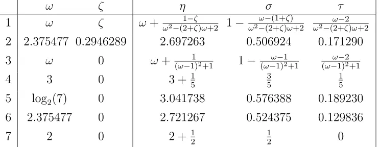
All of the above bit costs lead to total bit complexity of (nη_logkAk)1+o(1)

ω ζ η σ τ 1 ω ζ ω+ _ω2₋₍₂₊1−ζ_ζ)ω+2 1−

ω−(1+ζ)

ω2_{−(2+ζ)ω+2 ω}2₋₍₂₊ω−_ζ2_)ω+2

2 2.375477 0.2946289 2.697263 0.506924 0.171290

3 ω 0 ω+ 1

(ω−1)2₊₁ 1− _(ω−ω₁₎−12_{+1 (ω−}ω₁₎−22₊₁

4 3 0 3 + 1

5

3 5

1 5

5 log₂(7) 0 3.041738 0.576388 0.189230 6 2.375477 0 2.721267 0.524375 0.129836

7 2 0 2 + 1₂ 1₂ 0

Table 6.1: Determinantal bit/division-free complexity exponent η.

matrix multiplication schemes. Line 4 corresponds to the comments before Re-mark ReRe-mark 4.7 on page 115, and Line 5 uses Strassen’s original subquadratic matrix multiplication algorithm. Line 6 exhibits the slowdown without faster rectangular matrix multiplication algorithms. Line 7 is our complexity for a hypothetical quadratic matrix multiplication algorithm.

An issue arises whether the singularity certification in Step 0 of our algo-rithm can be accomplished at a matching or lower bit complexity than the ones given above for the determinant. We refer to possible approaches by Mulders and Storjohann (2004) and Storjohann (2004).

The above analysis applies to our algorithm in Section 5 and yields for the determinant and adjoint matrix a division-free complexity of O(n2.697263_{) ring}

operations. To our knowledge, this is the best-known to-date. For the division-free computation of the characteristic polynomial the homotopy inz is altered, because the computation of detF_XL(z),Y(λ) mod (zn+1_{, λ}n+1_{) in Step 4 (see}

Sec-tion 5) seems to require too many ring operaSec-tions. One instead computes

det(M −zAM) = det(I−zA) det(M) = ±zndet(1/zI −A)

by replacing A − M by AM in the original determinant algorithm. Since det(M) = ±1 one thus gets (the reverse of) the characteristic polynomial in O(n2.697263_{) ring operations as well.}

A Maple 7 worksheet that contains our exponent calculations is posted at

7. Integer characteristic polynomial and normal forms

As already seen in Section 5 and Section 6 over an abstract ring R, our de-terminant algorithm also computes the adjoint matrix and the characteristic polynomial. In the case of integer matrices, although differently from the alge-braic setting, the algorithm of Section 4 may also be extended to solving other problems. We briefly mention two extensions in the following. For A ∈ Zn×n

we shall first see that the algorithm leads to the characteristic polynomial of a preconditioning of A and consequently to the Smith normal form of A. We shall then see howF_XA,Y may be used for computing the Frobenius normal form of A and hence its characteristic polynomial. Note that the exponents in our bit complexity are of the same order than those discussed for the determinant problem in Table 6.1.

7.1. Smith normal form of integer matrices. A randomized Monte Carlo algorithm for computing the Smith normal formS∈Zn×n of an integer matrix A∈Zn×n of rankr may be designed by combining the algorithm of Section 4 with the approach of Giesbrecht (2001). Here we improve on the best previously known randomized algorithm of Eberlyet al. (2000). The current estimate for a deterministic computation of the form is (nω+1_logkAk)1+o(1) _(Storjohann

1996).

The Smith normal form over Z is defined in a way similar to what we have seen in Section 2.2 for polynomial matrices. The Smith formS is an equivalent diagonal matrix inZn×n_{, with diagonal elementss}

1, s2, . . . , sr,0, . . . ,0 such that si divides si−1 for 2≤ i≤r. Thesi’s are the invariant factors of A (Newman

1972).

Giesbrecht’s approach reduces the computation of S to the computation of the characteristic polynomials of matrices D₁(i)T(i)_D(i)

2 A for l = (logn +

log logkAk)1+o(1) _{random choices of diagonal matrices D}(i)

1 and D (i)

2 and of

Toeplitz matrices T(i)_{, 1 ≤ i ≤ l. The invariant factors may be computed}

from the coefficients of these characteristic polynomials. The preconditioning B ←D₁(i)T(i)_D(i)

2 Aensures that the minimum polynomialfB ofB is squarefree

(Giesbrecht 2001, Theorem 1.4) (see also Chen et al. 2002 for such precondi-tionings). Hence if ¯fB _{denotes the largest divisor of f}B _{such that ¯f}B_{(0) 6= 0,}

we have r = rankB = deg ¯fB _{which is −1 + degf}B _{if A is singular. By}

Theorem 2.12, for random X and Y we shall have, with high probability, ∆(λ) = det(F_XB,Y(λ)) = λk1_fB_{(λ) = λ}k2_f¯B_{(λ) for two positive integers k}

1

and k2 that depend on the rank and on the blocking factor m. The needed

characteristic polynomials λn−r_f¯B _{and then the Smith form are thus obtained}