A binary powering Schur algorithm for computing primary matrix roots

(1)

Numerical Algorithms manuscript No. (will be inserted by the editor)

A binary powering Schur algorithm for computing primary

matrix roots

Federico Greco · Bruno Iannazzo

Received: date / Accepted: date

Abstract An algorithm for computing primary roots of a nonsingular matrix A is presented. In particular, it computes the principal root of a real matrix having no nonpositive real eigenvalues, using real arithmetic. The algorithm is based on the Schur decomposition ofA and has an order of complexity lower than the customary Schur based algorithm, namely the Smith algorithm.

Keywords matrix pth root·matrix functions· Schur method· binary powering technique

Mathematics Subject Classification (2000) 65F30·15A15

1 Introduction

Let p be a positive integer. A primary pth root of a square matrix A ∈ Cn×n is a solution of the matrix equationXp−A= 0 that can be written as a polynomial ofA. IfAhas`distinct eigenvalues, sayλ1, . . . , λ`, none of which is zero, thenAhas exactly p`primarypth roots. They are obtained as

f(A) := 1 2πi

I γ

f(z)(zI−A)−1dz, (1)

wheref is any of thep` analytic functions defined on the spectrum ofA, denoted by σ(A) :={λ1, . . . , λ`}, and such thatf(z)p=zandγis a closed contour which encloses σ(A). The reason whyf(A) is a polynomial ofA is subtle and it is well explained in [10].

IfAhas no nonpositive real eigenvalues then there exists only one primarypth root whose eigenvalues lie in the sector

Sp={z∈C\ {0} : |arg(z)|< π/p}, (2)

Federico Greco, Bruno Iannazzo

Dipartimento di Matematica e Informatica, Universit`a di Perugia Via Vanvitelli 1, I-06123 Perugia, Italy

(2)

which is called principalpth root.

The main numerical problem is to compute the principal pth root of A, whose applications arise in finance or in the numerical computation of other matrix functions [8, 9, 15]. In particular if A is real and has no nonpositive real eigenvalues, then the principalpth root is proved to be real [8], and in order to compute it, it is preferable to have an algorithm which works entirely in real arithmetic.

The reliable algorithms are essentially of two kinds: 1. Algorithms based on matrix iterations;

2. Algorithms based on the Schur normal form.

In the first case, one uses a rational matrix iteration which converges to the principal pth root ofA. This approach is very complicated since the iterations usually do not depend continuously on the initial data, that is, if a perturbation on some iterate is introduced then it is potentially amplified by the subsequent steps and could result in numerical instability. Moreover, in the case p >2 the convergence properties, also in the scalar case, are hard to describe.

The first rational iteration used for the square root is the so-called Newton method Xk+1=12(Xk+Xk−1A), which was observed to be unstable by Laasonen [14], but the instability was first analyzed by Higham [6]. Some stable iterations have been proposed, the first of them is the Denman and Beavers iteration [2] and many others have followed [11, 17].

The case p >2 is more complicated. In order to have a general algorithm, some kind of preprocessing of the matrix A should be done. The first general and stable algorithm was given by Iannazzo [12] and some others have followed [3, 4, 13, 16]. The computational cost of these algorithms isO(n3log2p) arithmetic operations (ops) and the storage required isO(n2log₂p) real numbers.

The algorithms based on some matrix iteration show good numerical stability in the numerical tests, even if their behavior in the finite arithmetic for any matrix A is practically unpredictable and a thorough analysis is yet to be developed. Moreover, these algorithms compute just the principal pth root, and it is not clear if they can compute any of the primarypth roots ofAwith the same computational cost.

For the second class of algorithms, in order to compute a solution ofXp−A= 0, one computes the Schur normal form ofA, sayQ∗AQ=R, whereQis unitary andR is upper triangular and then solves the equationYp−R= 0 and deducesX=QY Q∗. Since Y is proved to be upper triangular, the equation Yp−R = 0 is solved by a recursion on the elements ofY [8].

In the important case in which Ais real, the real Schur form ofA is formed, say QTAQ=R, where Qis orthogonal andR is quasi-upper triangular, that is real and block upper triangular with diagonal blocks of size 1 or 2 according as they correspond to one real or a couple of complex conjugate eigenvalues, respectively. The equation Yp−R= 0 is solved by a recursion on the blocks ofY which is proved to have the same block structure asR. This approach works on the idea of the Schur-Parlett recurrence for computing general matrix functions. The casep= 2 was first developed by Bj¨orck and Hammarling [1] in the complex case and then by Higham [7] in the real case. Finally, the casep >2 was worked out by Smith [18].

The method developed by Smith has a cost ofO(n3p) ops and requires the storage ofO(n2p) real numbers. Ifpis composite, sayp=q1q2, it is thus convenient to form first theq1th root and then theq2th root ofA. However, ifpis prime, the cost of the method of Smith can be large and that makes the algorithm uneffective.

(3)

A nice feature of the Smith algorithm is that it has been proved to be backward stable, thus it is in some sense optimal in finite arithmetic. Moreover, it can compute any of the primarypth roots ofAwith the same cost.

We propose a new algorithm based on the Schur normal form of A whose cost is lowered to O(n2p+n3log2p) ops and the storage is lowered toO(np+n2log2p) real numbers. The proposed algorithm combines the advantages of being based on the Schur form and the low computational cost of the iterations.

The numerical tests show that the new algorithm reach the same numerical accu-racy as the one of Smith.

The paper is organized as follows. In Section 2 we describe and analyze the proposed method; in Section 3 we summarize the resulting algorithm; in Section 4 we discuss how to further reduce the cost of the algorithm; finally, in Section 5 we present some numerical experiments which confirm the reliability of the algorithm.

2 A Schur method based on the binary powering technique

One of the most used methods for computing the principal pth root, for p positive integer, of a real matrix A∈ Rn×n having no nonpositive real eigenvalues has been proposed by Smith in [18]. Since the principalpth root of such a matrix is proved to be real, the method is designed to work entirely in real arithmetics.

The idea of the algorithm is to compute the real Schur normal form of A, say QTAQ=R, whereQis orthogonal andRis real and quasi-upper triangular, namely the matrix is blockσ×σ, block upper triangular and itsσdiagonal blocks are real numbers or 2×2 real matrices corresponding to a couple of complex conjugate eigenvalues. Once the real Schur form is obtained, one applies the transformation to the equation

Xp=A, (3)

obtaining the new equation

Up=R, (4)

whereU=QTXQ. IfX is the principalpth root ofAthenU is the principalpth root of R as well, moreover, the matrix U is quasi-upper triangular with the same block structure asR(that follows from the fact that a primary pth root of a matrixAis a polynomial inA, see also [8]).

From a solution U of (4) one obtains a solution of (3) usingX =QU QT, so ifU is chosen to be the principalpth root ofR, sayU =R1/p then the principalpth root ofAisA1/p=QU QT (recall thatU andQU QT have the same eigenvalues).

The key point of the algorithm is the solution of (4) which is done by a clever recursion, employing the same idea as the methods of Bj¨orck and Hammarling [1] and Higham [6] for the matrix square root.

The recursion of Smith [18, 19] is obtained considering the sequence of matrices ( e V(0) =U, e V(k) = UVe(k−1) = Uk+1, k= 1, . . . , p−2, (5)

having the same quasi-triangular structure asU andR. The diagonal blocks ofU are obtained from thepth roots of the corresponding blocks ofRusing a simple formula:

(4)

ifUii is a 1×1 block, thenUii is the principalpth root of the scalarRii; ifUii is a 2×2 block corresponding to the complex conjugate eigenvaluesθ±iµ, then

Uii=αI+ β

µ(Rii−θI), (6)

whereIis the 2×2 identity matrix andα+iβis the principalpth root ofθ+iµ. The upper triangular part of U is obtained, a block column at a time, equating the (i, j) blocks in equation (5) (more details can be found in [8, 18]).

The main drawback of the Smith method is the high cost in terms of arithmetic operations (ops) and storage for large p, in particular it needs O(n3p) ops and the storage ofO(n2p) real numbers. The most expensive part is the computation of the elements of the intermediate matricesVe(k)and their storage. The idea of our algorithm is to use a recursion similar to the one of Smith but with less intermediate matrices obtaining an algorithm with similar features but less expensive. The proposed recursion is based on the binary powering decomposition of the integerp, that is

p =

blog₂pc

X k=0

bk2k, for a unique choice ofb0, . . . , bblog₂pc∈ {0,1}, (7)

whereb_blog₂pc = 1. Observe thatbi, fori= 0, . . . ,blog2pc, are the digits in the binary representation ofp.

We define also the sets

c(p) ={k : bk= 1}, c(p)+=c(p)\ {0}. (8) The set c(p) has cardinality m+ 1, for some nonnegative integer m, while the set c(p)+ coincides withc(p) ifpis even (that is 0 6∈c(p)) and has cardinalitym ifpis odd. Clearly,m+ 1 denotes the number of 1s comparing in the binary representation of p. Let c0, c1, . . . , cm be the sequence obtained by sorting the elements ofc(p) by decreasing order. Note that ifm >0, then

c0=blog2pc,

ch= max{k : k < ch−1, bk= 1}, h= 1, . . . , m,

(9) while ifm= 0, then the sequence contains just the termc0=blog2pc.

Since Up=R, R=Up= blog₂pc Y k=0 Ubk2k₌ m Y h=0 U2ch,

and it is possible to devise a method based on a sequence of c0+m = O(log2p) intermediate matrices from which construct a recursion for computingU.

We obtain the furtherc0matrices as follows (

V(0) = U

V(k) = V(k−1)·V(k−1) = U2k, k= 1, . . . , c0,

(10)

and the lattermmatrices as follows (

W(0) = V(c0)

(5)

whereW(m)=R.

The matricesV(k)andW(h)have the same block structure asR, being quasi-upper triangular. We denote the blocks of V(k) and W(h) by V_ij(k) and W_ij(h), respectively, where the indicesi, jgo from 1 toσ, whereσ2is the number of blocks in the partitioning ofR. Each choice ofiandjcould correspond to a 1×1, or to a 1×2, or to a 2×1, or to a 2×2 block, according to the quasi-triangular structure ofR.

The idea of the proposed method is to compute, using (10) and (11), the blocks of U, that isV(0), in the following order: first, compute the diagonal blocks of U, then compute the upper part ofU,V(k)andW(h)a column at a time from the bottom to the top. During the computation we need the diagonal blocks ofUq forq = 1, . . . , p. These blocks can be computed with a cost ofO(n2p) ops and a storage ofO(np) real numbers.

Relations (10) and (11) can be restated in terms of blocks, for eachi, j= 1, . . . , σ such thati6j, fork= 1, . . . , c0, and forh= 1, . . . , mone has

V_ij(k) = j X ξ=i V_iξ(k−1)V_ξj(k−1), W_ij(h) = j X ξ=i W_iξ(h−1)V(ch) ξj , (12)

while fori > jthe blocksV_ij(k)andW_ij(h)are zero for eachk.

In order to get useful formulae we isolate the terms containing the indicesiandj in the sum, obtaining

V_ii(k−1)V_ij(k−1)+V_ij(k−1)V_jj(k−1) = V_ij(k)−B_ij(k), (13) W_ii(h−1)V(ch) ij +V (ch) ij W (h−1) jj = W (h) ij −C (h) ij . (14)

whereB_ij(k), andC_ij(h)denote something which is already known when one is computing the blockUij, in fact, forj > i+ 1,

B_ij(k) = j−1 X ξ=i+1 V_iξ(k−1)V_ξj(k−1), C_ij(h) = j−1 X ξ=i+1 W_iξ(h−1)V(ch) ξj , and forj=i+ 1,B_ij(k)=C_ij(h)= 0.

Now we show how to use equations (13) and (14) in order to obtain a single equation from which recover Uij for each iand j. The construction of such equation is quite technical and will be done in the rest of the section.

LetA1 = {(0; 1; 0)}, and let

Ak = [ (r;s;t)∈Ak−1

{(r+ 2k−1;s;t),(r;s;t+ 2k−1)} ∪ {(0;k; 0)}, (15)

for any integerk >1.

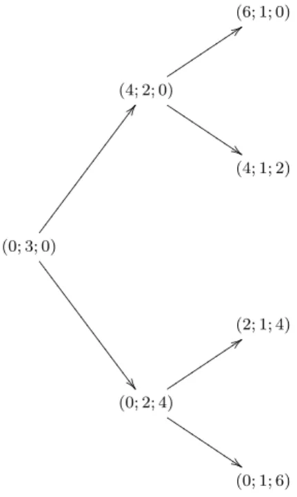
The set Ak contains 2k−1 triples; it can be easily shown that the following two properties completely describeAk:

(6)

(i) (0;k; 0)∈Ak holds;

(ii) If (r;s;t)∈Ak, ands >1, then (r+2s−1;s−1;t)∈Ak, and (r;s−1;t+2s−1)∈Ak. Property (i), and (ii) allow us to represent the elements inAk by a tree. In Figure 1 the tree in the casek= 3 is depicted.

(6; 1; 0) (4; 2; 0) : : t t t t t t t t t $ $ J J J J J J J J J (4; 1; 2) (0; 3; 0) C C 7 7 7 7 7 7 7 7 7 7 7 7 7 7 7 7 (2; 1; 4) (0; 2; 4) : : t t t t t t t t t $ $ J J J J J J J J J (0; 1; 6) Fig. 1 A tree representation ofA3

We first explain how the blocks of U can be constructed when p= 2k, then the general case is described. We recall that the algorithm will be used essentially only if pis a prime number, the casep= 2k is presented just for the sake of the clarity.

Let us illustrate what happens in the case p= 16 to better understand the case p= 2k. Observe that forp= 2k one needs only equation (10). Let us suppose that the diagonal blocksU_iiq for anyq= 0, . . . ,15 have been already computed. It follows from (13) applied fork= 4 that

V_ij(4) =V_ii(3)V_ij(3)+V_ij(3)V_jj(3)+B(4)_ij . Note thatB_ij(4)=Uii0B

(4) ij U

0

jj, and it can be associated with the triple (0; 4; 0) belonging to the first level in the tree corresponding to A4. Let us consider the termV_ii(3)V_ij(3), it follows from (13) applied fork= 3 that

V_ii(3)V_ij(3) =Uii8 V_ii(2)V_ij(2)+V_ij(2)V_jj(2)+Uii8B (3) ij . Note thatUii8B (3) ij =U 8 iiB (3) ij U 0

jj, and that it can be associated with the triple (8; 3; 0) belonging to a part of the second level of the tree corresponding toA4. Clearly, the

(7)

triple (0; 3; 8) appears when we substitute (13) fork = 3 inV_ij(3)V_jj(3). Recalling that V_ii(2) =U_ii4, and thatV_jj(2) =U_jj4, we obtain by making use of (13) applied fork= 2 that Uii12V (2) ij +U 8 iiV (2) ij U 4 jj =Uii12 V_ii(1)V_ij(1)+V_ij(1)V_jj(1) +Uii12B (2) ij +Uii8 V_ii(1)V_ij(1)+V_ij(1)V_jj(1)Ujj4 +U 8 iiB (2) ij U 4 jj. By arguing as above, the two termsU_ii12B(2)_ij and U_ii8B_ij(2)U_jj4 are associated with the triples (12; 2; 0), and (8; 2; 4), respectively. The other two triples belonging to the third level of the tree corresponding toA4appear, for symmetry, when we simplifyV_ij(3)V_jj(3). Remembering thatV_ii(1)=U_ii2, and thatV_jj(1)=U_jj2, we obtain by making use of (13) fork= 1 that Uii14V (1) ij =U 15 ii V (0) ij +U 14 ii V (0) ij Ujj+U 14 ii B (1) ij , Uii12V (1) ij U 2 jj =Uii13V (0) ij U 2 jj+Uii12V (0) ij U 3 jj+Uii12B (1) ij U 2 jj, Uii10V (1) ij U 4 jj =Uii11V (0) ij U 4 jj+Uii10V (0) ij U 5 jj+Uii10B (1) ij U 4 jj, Uii8V (1) ij U 6 jj =U 9 iiV (0) ij U 6 jj+U 8 iiV (0) ij U 7 jj+U 8 iiB (1) ij U 6 jj,

which make appear the missing terms inA4. In general, it holds the following result. Lemma 1 Ifp= 2c0_{, for some positive integer}_c_{0, then}

Rij = p−1 X q=0 U_iiqV_ij(0)U_jjp−1−q+ X (r;s;t)∈Ac0 UiirB (s) ij U t jj. (16)

Proof The claim is proved by induction onc0. Let us supposec0= 1, from (13) applied fork= 1 it follows that

Rij =V (1) ij = V (0) ii V (0) ij +V (0) ij V (0) jj +B (1) ij . SinceV_ii(0)=Uii,V (0)

jj =Ujj, andA1 = {(0; 1; 0)}, the claim trivially follows. Let us assume the claim for c0=c >0, and let us prove it forc0=c+ 1. From (13) applied fork=c+ 1 it follows that

Rij = Vij(c+1) = V (c) ii V (c) ij +V (c) ij V (c) jj +B (c+1) ij .

By making use of inductive hypothesis and observing thatV_ii(c)=U_ii2c, andV_jj(c)=U_jj2c, the above equation can be written as

Rij = U2 c ii   2c₋₁ X q=0 U_iiqV_ij(0)U_jj2c−1−q+ X (r;s;t)∈Ac UiirB (s) ij U t jj   +   2c₋₁ X q=0 U_iiqV_ij(0)U_jj2c−1−q+ X (r;s;t)∈Ac UiirB (s) ij U t jj  U 2c jj +B (c+1) ij = 2c₋₁ X q=0 U_iiq+2cV_ij(0)U_jj2c−1−q+U_iiqV_ij(0)U_jj2c−1−q+2c + X (r;s;t)∈Ac U_iir+2cB(s)_ij Ujjt +UiirB (s) ij U t+2c jj +Uii0B (c+1) ij U 0 jj.

(8)

The former term of the last expression can be written as 2c+1−1

X q=0

U_iiqV_ij(0)U_jj2c+1−1−q, while the latter term of the last expression can be rearranged as X

(r;s;t)∈Ac+1 UiirB (s) ij U t jj as a consequence of the definition ofAk fork=c+ 1. The claim thus follows.

Note that the two sums involved inRij havep, and 2c0−1 =p−1 terms, respec-tively.

Lemma 1 provides a basis for an algorithm for the 2kth root of a matrix. We need the use of the Kronecker notation [10], that is the Kronecker product, the vec operator which stacks the columns of a matrix in a long vector and the well-know relation vec(AXB) = (BT⊗A) vec(X), forA, X, Bmatrices of suitable sizes.

Using the Kronecker notation andV_ij(0)=Uij, equation (16) can be rewritten as   p−1 X q=0 U_jjp−1−q T ⊗U_iiq  vec(Uij) = vec  Rij− X (r;s;t)∈Ac0 UiirB (s) ij U t jj  , (17)

which is a linear system of size at most 4, whose unknown is vec(Uij), and the matrix coefficient and the right hand side are known quantities since they involve already computed blocks. The solution is unique as the matrix coefficient is the transpose of the one appearing in the Smith algorithm which is proved to be nonsingular [18].

In order to go further to the case in which p is arbitrary, let us illustrate what happens for p= 23, wherem= 3, c0= 4, c1= 2,c2 = 1,c3 = 0. By making use of (14) fork= 3, we have that

W_ij(3) = W_ii(2)V_ij(0)+W_ij(2)V_jj(0)+C_ij(3) = Uii22V (0) ij +W

(2)

ij Ujj+Cij(3), where we have used thatW_ii(2)=U_ii2c0+2c1+2c2 =U_ii22, and thatV_jj(0)=Ujj. The only summand which needs to be further reduced is the second one; according to (14), for k= 2 we have that W_ij(2)Ujj = (W (1) ii V (1) ij +W (1) ij V (1) jj )Ujj+C (2) ij Ujj = Uii20V (1) ij Ujj+Wij(1)U 3 jj+C (2) ij Ujj,

where we have used that W_ii(1) = U_ii2c0+2c1 = U_ii20, and V_jj(1) = U_jj2. Moreover, it follows from Lemma 1 that

V_ij(1) = 1 X q=0 U_iiqV_ij(0)U_jj1−q+ X (r;s;t)∈A1 UiirB (s) ij U t jj, hence, Uii20V (1) ij Ujj = Uii20   1 X q=0 U_iiqV_ij(0)U_jj1−q  Ujj+Uii20   X (r;s;t)∈A1 UiirB (s) ij U t jj  Ujj.

(9)

According to (14), fork= 1, we have that W_ij(1)Ujj3 = W (0) ii V (2) ij U 3 jj+W (0) ij V (2) jj U 3 jj+C (1) ij U 3 jj = Uii16V (2) ij U 3 jj+W (0) ij U 7 jj+C (1) ij U 3 jj.

Note that W_ii(0) = U_ii2c0 = U_ii16, and that V_jj(2) = U_jj4. Moreover, from Lemma 1 it follows that V_ij(2) = 3 X q=0 U_iiqV_ij(0)U_jj3−q+ X (r;s;t)∈A2 UiirB (s) ij U t jj, hence, Uii16V (2) ij U 3 jj = U 16 ii   3 X q=0 U_iiqV_ij(0)U_jj3−q  U 3 jj+U 16 ii   X (r;s;t)∈A2 UiirB (s) ij U t jj  U 3 jj.

On the other hand,

W_ij(0)Ujj7 = V (4) ij U 7 jj =   15 X q=0 U_iiqV_ij(0)U_jj15−q  U 7 jj+   X (r;s;t)∈A4 UiirB (s) ij U t jj  U 7 jj,

by making use of Lemma 1 forc0= 4, and of (14) fork= 0. All terms involvingV_ij(0)can be grouped as follows

22 X q=0

U_iiqV_ij(0)U_jj22−q,

while the remaining terms can be divided into two summands. The first one containing C_ij(h),i, j= 1, . . . , σ, can be written as

3 X h=1

C_ij(h)U_jj2ch+1+···+2c3,

whereU_jj2ch+1+···+2c3 denotes the identity matrix forh= 3. The second one referring to theB(k)_ij ’s, can be written as

X h∈c(23)+ U_ii23−2ch−···−2c3   X (r;s;t)∈A_ch UiirB (s) ij U t jj  U 2ch+1₊_···₊₂c3 jj ,

wherec(23)+is the set{4,2,1}, according to definition (8). Now we give the main result of this section.

(10)

Theorem 1 Letp= m X h=0

2ch _{be a positive integer greater than}₁_and_c(p)+ _{as in} ₍₈₎_. Then Rij = p−1 X q=0 U_iiqV_ij(0)U_jjp−1−q + m X h=1 C_ij(h)U_jj2ch+1+···+2cm + X h∈c(p)+ U_iip−2ch−···−2cm   X (r;s;t)∈A_ch UiirB (s) ij U t jj  U 2ch+1+···+2cm jj , (18)

where, forh=m,U_jj2ch+1+···+2cm denotes the identity matrix, form= 0 the second summand on the right hand side of (18)is the zero matrix and the third summand on the right hand side of (18)is the zero matrix whenc(p)+ is the empty set.

Proof The claim is done by induction onm. Let us assumem= 0, hence,p= 2c0_{, for}

some positive integerc0. The claim thus follows from Lemma 1.

Let us assume the claim form=µ, and let us prove it form=µ+ 1, note that in this casep=

µ X h=0

2ch_{+ 2}cµ+1_{. Let}_p0 _{denote the integer}

µ X h=0

2ch_{, thus}_p₌_p0_{+ 2}cµ+1_.

It follows from (11) applied forh=µ+ 1 that Rij = W (µ+1) ij = W (µ) ii V (cµ+1) ij +W (µ) ij V (cµ+1) jj +C (µ+1) ij . Note that W_ii(µ) =U_iip0, and thatV(cµ+1)

jj =U

2cµ+1

jj . By making use of the induction hypothesis forW_ij(µ), Rij = Up 0 iiV (cµ+1) ij + p 0₋₁ X q=0 U_iiqV_ij(0)U_jjp0−1−q + µ X h=1 C_ij(h)U_jj2ch+1+···+2cµ + X h∈c(p0₎+ U_iip0−2ch−···−2cµ   X (r;s;t)∈A_ch UiirB (s) ij U t jj  U 2ch+1+···+2cµ jj Ujj2cµ+1+C (µ+1) ij .

As a consequence of the relationp=p0+ 2cµ+1_{, we have that}

Rij = Up 0 iiV (cµ+1) ij + p0−1 X q=0 U_iiqV_ij(0)U_jjp−1−q + µ X h=1 C_ij(h)U_jj2ch+1+···+2cµ+2cµ+1+C_ij(µ+1) + X h∈c(p0₎+ U_iip−2ch−···−2cµ−2cµ+1   X (r;s;t)∈A_ch UiirB (s) ij U t jj  U 2ch+1₊_···₊₂cµ₊₂cµ+1 jj .

Asµ+ 1 =m,U_jj2cµ+2+···+2cµ+1 denotes the identity matrix. Hence, the termC[p] := Pµ h=1C (h) ij U 2ch+1+···+2cµ+1 jj +C (µ+1)

ij is equal to the second sum in the right hand side of equation (18) form=µ+ 1.

In order to complete the proof, we distinguish two cases:cµ+1= 0 andcµ+1>0 which correspond topodd andpeven, respectively.

(11)

Ifcµ+1= 0, thenV_ij(cµ+1)=V_ij(0)=Uij, andU2 cµ+1 jj =Ujj hold, hence, Rij = Up 0 iiV (0) ij + p0−1 X q=0 U_iiqV_ij(0)U_jjp−1−q +C[p] (19) + X h∈c(p0₎+ U_iip−2ch−···−2cµ−2cµ+1   X (r;s;t)∈A_ch UiirB (s) ij U t jj  U 2ch+1+···+2cµ₊₂cµ+1 jj .

Sincep=p0+ 1, the first two summands of the right hand side of (19) can be written as

p−1 X q=0

U_iiqV_ij(0)U_jjp−1−q, which corresponds to the first sum in the the right hand side of equation (18) form=µ+ 1.

Finally, noting that c(p)+ =c(p0)+, the second row in equation (19) corresponds to the third sum in the the right hand side of equation (18) form=µ+ 1.

The claim thus follows in the casecµ+1= 0. Suppose, now, thatcµ+1>0. Let us computeV

(cµ+1)

ij using Lemma 1 forc=cµ+1. Hence, Rij = Up 0 ii 2cµ+1−1 X q=0 U_iiqV_ij(0)U_jj2cµ+1−1−q+ X (r;s;t)∈A_cµ₊₁ UiirB (s) ij U t jj + p0₋₁ X q=0 U_iiqV_ij(0)U_jjp−1−q +C[p] + X h∈c(p0₎+ U_iip−2ch−···−2cµ−2cµ+1   X (r;s;t)∈A_ch UiirB (s) ij U t jj  U 2ch+1+···+2cµ₊₂cµ+1 jj . Sincep=p0+ 2cµ+1_, Up 0 ii 2cµ+1₋₁ X q=0 U_iiqV_ij(0)U_jj2cµ+1−1−q+ p0−1 X q=0 U_iiqV_ij(0)U_jjp−1−q = p−1 X q=0 U_iiqV_ij(0)U_jjp−1−q,

thus, the first sum in the the right hand side of equation (18) form=µ+ 1 has been obtained. Moreover, U_iip0 X (r;s;t)∈A_cµ₊₁ UiirB (s) ij U t jj = U p−2cµ+1 ii X (r;s;t)∈A_cµ₊₁ UiirB (s) ij U t jj Ujj0

Noting thatc(p)+=c(p0)+∪ {µ+ 1}, the remaining terms can be written as

X h∈c(p)+ U_iip−2ch−···−2cµ−2cµ+1   X (r;s;t)∈A_ch UiirB (s) ij U t jj  U 2ch+1+···+2cµ₊₂cµ+1 jj .

(12)

Note that the first sums involved inRij according to Theorem 1 haspsummands. The second one hasmsummands, and the third one hasP

h∈c(p)+(2ch−1) terms. In

particular,

m+ X

h∈c(p)+

(2ch₋_{1) =} _p₋₁

in both casescm= 0, andcm>0.

3 The algorithm

We summarize the algorithm for computing the principal pth root of a real matrix having no nonpositive real eigenvalues.

Algorithm 1(Binary powering Schur algorithm for the principal pth root of a real matrixA)

1. compute a real Schur decompositionA=QRQT, whereR is blockσ×σ

2. computeb0, . . . , bblog₂pc andc0, . . . , cmin the binary decomposition ofpas in (7) and (9)

3. forj= 1 :σ

4. computeUjj=R 1/p

jj (using (6) if the size ofUjj is 2) 5. forq= 0 :p−1 computeD_j(q)=U_jjq, end

6. fork= 0 :c0 setV_jj(k)=U2 k jj, end 7. W_jj(0)=V(c0) jj 8. forh= 1 :msetW_jj(h)=W_jj(h−1)V(ch) jj , end 9. fori=j−1 :−1 : 1 10. fork= 1 :c0 11. Bk=Pj`=i+1−1 V (k−1) iξ V (k−1) ξj 12. end 13. forh= 1 :m 14. Ch= Pj−1 `=i+1W (h) iξ V (ch) ξj 15. end 16. solvePp_q=0−1D(q)_i UijD (p−q−1) j =Rij−Pmh=1ChD (2ch+1+···+2cm₎ j −P h∈c(p)+D (p−2ch−···−2cm) i h P (r;s;t)∈A_chD (r) i BsD (t) j i D_j(2ch+1+···+2cm) with respect toUij 17. V_ij(0)=Uij 18. fork= 1 :c0 19. V_ij(k)=Bk+V (k−1) ii V (k−1) ij +V (k−1) ij V (k−1) jj 20. end 21. W_ij(0)=V(c0) ij 22. forh= 1 :m 23. W_ij(h)=Ch+W (h−1) ii V (ch) ij +W (h−1) ij V (ch) jj 24. end 25. end 26. end 27. computeA1/p=QTU Q.

(13)

In Steps 11, 14 and 16, we assume that a void sum is the zero matrix, while in Step 16 we assume that given a matrixM,M2ch+1+···+2cm is the identity matrix for h=m.

Let us analyze the computational cost of Algorithm 1. We can assume that σ = O(n),c0=O(log2p) andm=O(log2p). Step 5 requires the computation ofppowers of s blocks of size at most 2, the cost is O(np) ops. Steps 6–8 are obtained with no more cost. Steps 10–12 require c0 sums from i+ 1 toj−1 for each i < j−1, the resulting cost isO(n3log₂p) ops, the same cost is required for Steps 13–15. Forming the coefficients and solving the equation at Step 16 requiresO(n2p) ops, since the sum on the right hand side contains no more than 2 log₂pterms. Finally, the cost of Steps 18–20 and 22–24 isO(n2log2p).

In summary the cost of the algorithm isO(n2p+n3log2p) ops which asymptotically favorably compares to the Smith method whose cost isO(n3p) ops. Algorithm 1 requires less operations also for smallporn and this leads to a faster computation as we will show in Section 5. The cost could be further lowered as suggested in Section 4.

Consider now the cost in memory. The main expenses are due: to the storage of V(k),W(h)which areO(log2p)n×nmatrices for a total ofO(n2log2p) real numbers; to the storage of the block diagonal ofUq, namely, the blocksD(q)_j , wherej= 1, . . . , σ andq= 0, . . . , p−1 for a total ofO(np) real numbers.

In summary the algorithm requires the storage ofO(np+n2log₂p) real numbers.

Algorithm 1 can be slightly modified to work with the complex Schur form as well, in that case one gets the principalpth root of a complex matrix.

More generally the algorithm can be used to compute any primarypth root of a nonsingular matrixA, by choosing for each eigenvalue the desired pth root at Step 4, with the restriction that the same branch of thepth root function must be chosen for repeated eigenvalues.

If two different branches of thepth root are chosen for the same eigenvalue appear-ing in two different blocks, then the linear matrix equation at Step 18 admits no unique solution, and Algorithm 1 fails. However, in that case the resultingpth root would be nonprimary.

4 Possible further improvements

Algorithm 1 has a computational cost which isO(n2p+n3log2p) ops and needs the storage of O(np+n2log2p) real numbers. The linear dependence on pis bothering since the algorithms for the matrixpth root based on matrix iterations depend only on the logarithm ofp. It is possible to reduce further the computational cost of Algorithm 1.

The storage ofO(np) real numbers is due to the need of all the powers ofUii, say U_iiq, fori= 1, . . . , σandq= 1, . . . , p.

The computational cost ofO(n2p) ops is due to the solution of the matrix equations p−1 X q=0 U_iiqUijUjjp−1−q=Rij − m X h=1 C_ij(h)U_jj2ch+1+···+2cm (20) − X h∈c(p)+ U_iip−2ch−···−2cm   X (r;s;t)∈A_ch UiirB (s) ij U t jj  U 2ch+1+···+2cm jj ,

(14)

with respect toUij, for eachiandj.

We will explain how to reduce these costs for fixediandj. First, we compute and storeλk for any eigenvalueλofU, and for

k= 2,4, . . . ,2c0_,

k=p−2ch_{− · · · −}₂cm_, _h_{= 1, . . . , m,} k= 2ch+1₊_{· · ·}_{+ 2}cm_, _h_{= 1, . . . , m}₋_1, for a total amount ofO(log2p) values ofk.

Then, observe that ifRii is a scalarµi, thenUii=µi1/p =:λi, thus,Uiik =λki; if Rii is a 2×2 real matrix corresponding to the couple of complex eigenvalues θ±iµ, then its principal pth root Uii is obtained from the principal pth root of the scalar θ+iµthat isα+iβby formula (6). In a similar manner ifα(k)+iβ(k):= (α+iβ)k, then it is easy to see that

Uiik=α (k)

I+β (k)

µ (Rii−θI). (21)

Now, we can proceed in removing the linear term in p in the asymptotic costs. First, we explain how to construct the matrix coefficient

Mij:= p−1 X q=0 U_jjp−q−1 T ⊗U_iiq

withO(log₂p) ops.

Let λi =θi+iµi be one of the two eigenvalues ofUii and letλqi =α (q) i +iβ

(q) i , forq= 1, . . . , p−1, be the corresponding eigenvalue ofU_iiq, then using (21) the matrix coefficient becomes Mij =   p−1 X q=0 α(p_j −q−1)α(q)_i  I+   p−1 X q=0 β(p_j −q−1)α(q)_i   (Rjj−θjI)T⊗I µj +   p−1 X q=0 α(p_j −q−1)β_i(q)   I⊗(Rii−θiI) µi +   p−1 X q=0 β_j(p−q−1)β_i(q)   (Rjj−θjI)T⊗(Rii−θiI) µiµj , where, forλi6=λj, p−1 X q=0 α(p_j−q−1)α(q)_i =1 2 Re λp_i −λp_j λi−λj ! + Re λ p i −λ p j λi−λj !! , p−1 X q=0 β_j(p−q−1)α(q)_i =1 2 Im λp_i −λp_j λi−λj ! + Im λ p i −λ p j λi−λj !! , p−1 X q=0 α(p_j −q−1)β(q)_i =1 2 Im λp_i −λp_j λi−λj ! −Im λ p i −λ p j λi−λj !! , p−1 X q=0 β_j(p−q−1)β(q)_i =1 2 Re λp_i −λp_j λi−λj ! −Re λ p i −λ p j λi−λj !! ,

(15)

while forλi=λj it holds that λp_i−λp_j λi−λj =pλp_i−1.

Thus, for computing Mij one needs just thepth power of the eigenvalues of A, which have been already computed, and then performing a fixed number of arithmetic operations.

The second summand on the right hand side of (20) is a sum of m =O(log2p) terms. It can be computed withO(log2p) ops, since λ2

ch+1+···+2cm

j and, in view of

formula (21),U_jj2ch+1+···+2cm are known for eachh= 1, . . . , m.

Finally, we discuss how to compute inO(log22p) the last summand on right hand side of equation (20), that is,

X h∈c(p)+ U_iip−2ch−···−2cm   X (r;s;t)∈A_ch UiirB (s) ij U t jj  U 2ch+1+···+2cm jj . (22)

The cardinality ofc(p)+isO(log₂p), so, in order to obtain a total cost ofO(log2₂p) ops we need to compute the sum P

(r;s;t)∈A_chUiirB (s) ij U

t

jj in O(log2p) ops and the pre-multiplication by U_iip−2ch−···−2cm and the post-multiplication by U_jj2ch+1+···+2cm in O(1) ops. The latter two tasks follow from the fact that we already knowλp_i−2ch−···−2cm andλ2_jch+1+···+2cm and from the use of (21).

To conclude, we rewriteP

(r;s;t)∈A_chUiirB (s) ij U

t

jjin the equivalent form ch X s=1 X r,t (r,s,t)∈A_ch (Ujjt)T⊗Uiir vec(B_ij(s)), (23)

where the matrixP

(U_jjt )T ⊗U_iir is computed by a trick similar to the one used for Mij, by using only the known values ofλki andλkj.

For instance forA3(compare Figure 1) one must compute the matrices

(Ujj6)T ⊗I+ (Ujj4)T ⊗Uii2+ (Ujj2)T ⊗Uii4+I⊗Uii2, (Ujj4)

T

⊗I+I⊗Uii4.

If the matrices are 1×1, i.e.Uii=λi,Ujj=λj andλi6=λj, then the computation is reduced to p/2−1 X q=1 λ2(p_j −q−1)λ2q_i = λ p i −λ p j λ2 i −λ2j and λ4j+λ4i.

A drawback of this approach is that it is based on the simplification p−1 X q=0 λq_iλp_j−q−1=λ p i −λ p j λi−λj ,

computing the right hand side requires a lower computational cost, but is less numer-ically stable.

An open problem is the possibility to rearrange these ideas in a way such that the resulting algorithm is stable.

(16)

5 Numerical experiments

The analysis of the cost of Algorithm 1 of Section 3 both in terms of arithmetic op-erations and storage shows that it is asymptotically less expensive than the method proposed by Smith. We show by some numerical tests that in practice Algorithm 1 is faster than the one of Smith also for moderate values ofp, moreover, the two algorithms reach the same numerical accuracy. For smallpsuch as 2 or 3 the new algorithm does not give any advantage with respect to the one of Smith, on the contrary the latter in most cases is a bit faster in terms of CPU time.

The tests are performed on Matlab6, with unit roundoff 2−53 ≈ 1.1×10−16, where for the Smith method the implementation rootpm_real of Higham’s Matrix Function Toolbox [5] is used and for the new algorithm the implementation can be found at [20].

We compare the performance of the two algorithms on some test matrices. In particular the CPU time required for the execution of the two algorithms is computed and the accuracy is estimated in terms of the quantity

ρA(X) :=e kA−Xepk kXek Pp−1 i=0(Xep−1−i)T⊗Xei ,

whereXeis the computedpth root ofAandk·kis any matrix norm (in our tests we used the Frobenius norm denoted byk·kF). In [8], the quantityρAis proved to be a measure of accuracy more realistic than the norm of the relative residual, saykXep−Ak/kAk. To better describe the numerical properties of the methods we also compute the quantity β(U) =kUkp₂/kRk2, where U is the computed root of the (quasi) triangular matrix R from the Schur decomposition ofA, this quantity has been introduced in [19] as a measure of stability.

The results are summarized in Table 1, where n is the size of the matrices and “time” is the CPU time (in seconds) computed by_Matlab. If not otherwise stated we always compute the principalpth root.

Test 1 We consider the quasi upper triangular matrix

A=     1 1 1 1 0 2 1 1 0 0 1 −1 0 0 1 1     ,

and compute its principalpth root for some values of p. Since the difference between Smith’s algorithm and Algorithm 1 is the recursion used to compute thepth root of a (quasi) triangular matrix, the test is suitable to compare the accuracy and the CPU time of the two algorithms.

Test 2 We consider a 8×8 random stochastic matrix having no nonpositive real eigenvalues, which may be assumed to be the transition matrix relative to a period of one year in a Markov model [8, 9]. If one needs the transition matrix for one day, then a 365th root of A is required. Observe that 365 = 73·5 so it is enough to compute the 73th root followed by the 5th root. The average speedup of computing the 73th root of Awith Algorithm 1 with respect to the one of Smith is 9, while the residual ρA is essentially the same. For large p, the speedup increases further, for instance, if one computes the 521th root ofA, the speedup is 60. The value of β(U) is moderate and it is the same for both algorithms.

(17)

Test 3 ([19]) We consider the matrix A=     1.0000−1.0000−1.0000 −1.000 0 1.3000 −1.0000−1.0000 0 0 1.7000 −1.000 0 0 0 2.0000     ,

and compute its non principal 8th root

X=     1.0000 6.7778 17.091 36.469 0 −1.0333−5.2548−17.707 0 0 1.0686 7.1970 0 0 0 −1.0905     ,

for which β is large. Also in that case the two algorithms give the same numerical results.

Test 4 We consider the 10×10 Frank matrix, from_Matlabgalleryfunction, a matrix with ill-conditioned eigenvalues and for which the value ofβand the condition number of the matrix roots are rather large.

Test n p Smith Algorithm 1

β(U) ρA(Xe) time β(U) ρA(Xe) time 1 4 11 1.06 2.78·10−17 _<₀_.₀₂ ₁_.₀₆ ₁_.₉₈_·₁₀−17 _<₀_.₀₂ 4 101 1.06 5.21·10−17 _0.58 ₁_.₀₆ ₅_.₂₁_·₁₀−17 _0.05 4 1001 1.06 4.84·10−17 ₄₃ ₁_.₀₆ ₄_.₈₄_·₁₀−17 _0.34 2 8 73 60.6 5.34·10−16 _0.91 ₆₀_.₆ ₅_.₃₆_·₁₀−16 _0.094 8 521 61.0 6.02·10−16 ₄₀ ₆₁_.₀ ₅_.₉₈_·₁₀−16 _0.70 3 4 8 6.56·1012 ₆_.₅₆_·₁₀−19 _<₀_.₀₂ ₆_.₅₆_·₁₀12 ₈_.₃₄_·₁₀−19 _<₀_.₀₂ 4 10 11 6.18·1032 4.16·10−20 0.30 6.18·1032 4.67·10−20 0.062 Table 1 Comparison between Smith’s algorithm and Algorithm 1 of Section 3 for some test matrices.

Acknowledgments

We would like to thank Prof. N. J. Higham and the anonymous referees for their helpful comments which improved the presentation.

References

1. ˚A. Bj¨orck and S. Hammarling. A Schur method for the square root of a matrix. Linear Algebra Appl., 52/53:127–140, 1983.

2. E. D. Denman and A. N. Beavers, Jr. The matrix sign function and computations in systems. Appl. Math. Comput., 2(1):63–94, 1976.

3. C.-H. Guo. On Newton’s method and Halley’s method for the principal pth root of a matrix.Linear Algebra Appl. to appear.

(18)

4. C.-H. Guo and N. J. Higham. A Schur–Newton method for the matrixpth root and its inverse. SIAM J. Matrix Anal. Appl., 28(3):788–804, 2006.

5. N. J. Higham. The Matrix Function Toolbox. http://www.ma.man.ac.uk/~higham/ mctoolbox(Retrieved on November 3, 2009).

6. N. J. Higham. Newton’s method for the matrix square root. Math. Comp., 46(174):537– 549, 1986.

7. N. J. Higham. Computing real square roots of a real matrix. Linear Algebra Appl., 88/89:405–430, 1987.

8. N. J. Higham. Functions of Matrices: Theory and Computation. Society for Industrial and Applied Mathematics, Philadelphia, PA, USA, 2008.

9. N. J. Higham and L. Lin. Onpth roots of stochastic matrices. MIMS EPrint 2009.21, Manchester Institute for Mathematical Sciences, The University of Manchester, UK, Mar. 2009.

10. R. A. Horn and C. R. Johnson. Topics in Matrix Analysis. Cambridge University Press, Cambridge, 1994. Corrected reprint of the 1991 original.

11. B. Iannazzo. A note on computing the matrix square root. Calcolo, 40(4):273–283, 2003. 12. B. Iannazzo. On the Newton method for the matrixpth root. SIAM J. Matrix Anal.

Appl., 28(2):503–523, 2006.

13. B. Iannazzo. A family of rational iterations and its application to the computation of the matrixpth root.SIAM J. Matrix Anal. Appl., 30(4):1445–1462, 2008.

14. P. Laasonen. On the iterative solution of the matrix equationAX2₋_I_{= 0.}_{Math. Tables} Aids Comput., 12:109–116, 1958.

15. B. Laszkiewicz and K. Zi¸etak. Algorithms for the matrix sector function.Electron. Trans. Numer. Anal. To appear.

16. B. Laszkiewicz and K. Zi¸etak. A Pad´e family of iterations for the matrix sector function and the matrix pth root.Numer. Linear Alg. Appl. DOI: 10.1002/nla.656.

17. B. Meini. The matrix square root from a new functional perspective: theoretical results and computational issues. SIAM J. Matrix Anal. Appl., 26(2):362–376, 2004/05. 18. M. I. Smith. A Schur algorithm for computing matrixpth roots. SIAM J. Matrix Anal.

Appl., 24(4):971–989, 2003.

19. M. I. Smith. Numerical Computation of Matrix Functions. PhD thesis, University of Manchester, Manchester, England, September 2002.