Improving the structural
dynamics of slender
beam-like structures
A Ph.D. thesis
by
Christopher Stuart Anderson
Supervised by Dr S. Eren Semercigil
and Dr Özden F. Turan
Victoria University of Technology
School of the Built Environment
Summary and Significance
This project explores a novel technique for the vibration control of slender
beam-like flexible structures. For this purpose, a new method is developed
based on minor structural modifications. Three applications are chosen to
demonstrate the new method. The first is the sensing wire oscillations of a
hot-wire probe. The second application is the problem of tool chatter due to
milling tool vibration, while the third application is the bending of an arrow as it
is released from a bow. Although these applications sound quite different,
they are in fact similar problems dynamically. They are related to the forced
transverse structural vibrations of slender beams. For all applications, the
external force input is of a broadband nature in frequency, similar to a white
noise excitation. This force excites the slender beams into large amplitude
resonance which in the case of a hot-wire probe, causes measurement
inaccuracies, for milling, causes rough surface finish and slower machining
times, whereas for archery causes reduced accuracy. The choice of the
particular problems to demonstrate the effectiveness of the technique is due
to the current research interests and available expertise in this area in the
School of the Built Environment at Victoria University. However, the methods
developed through the course of this research are general methods applicable
ACKNOWLEDGMENTS
I would like to thank a number of people for their contribution, assistance and support.
Firstly to my parents, you made me who I am and for that I thank you. I thank my wife Fiona for her support and understanding. My brother, Jeremy also offered valuable support and experience after completing his own PhD.
My Grandfather-in-law, Ken, gave me inspiration and an enthusiastic thirst for knowledge. I knew him for 9 years before he passed away. I am grateful to have known him and thankful for his interest in my research.
Victoria University of Technology provided me a platform of resources, staff and experience for me to conduct my research. The Postgraduate studies unit provide valuable support to all postgraduate students. The staff within the School of the Built Environment were all extremely helpful.
I received an Australian Postgraduate Award scholarship to conduct my research and am grateful for this financial support.
Finally, I would like to sincerely thank my supervisors. Dr S. Eren Semercigil and Associate Professor Özden F. Turan were ideal supervisors. They gave me the direction I needed whilst allowing me the freedom I desired. Their experience and knowledge was an asset. I can only hope that some of it wore off onto me.
TABLE OF CONTENTS
Summary………..………...…ii
Acknowledgments………..……….…iv
Table of Contents………..……….……...………v
List of Tables..………...vi
List of Figures……….……….vii
Chapter 1 INTRODUCTION... 1
1.1 Existing Forms of Vibration Control ...1
Chapter 2 PROPOSED CONTROL TECHNIQUE ... 7
2.1 Introduction...7
2.2 Numerical Analysis of Slender Beam Geometries ...12
2.3 Discussion of Scaling in Frequency Plots ...30
2.3.1 Scaling Using Mass ...33
2.3.2 Scaling Using Individual Standard Beam Equations...35
2.4 Conclusions ...40
Chapter 3 SENSING WIRE VIBRATION OF HOT-WIRE PROBES ... 41
3.1 Introduction...41
3.2 Earlier Work...45
3.3 Numerical Modelling ...48
3.3.1 Numerical Model ...49
3.3.2 Numerical Predictions...51
3.3.3 Effect of L/d ...58
3.4 Scaled-up Experimental Verification...61
3.4.1 Experimental Setup ...61
3.4.2 Scaled-Up Experimental Results...65
3.5 Actual Size Experimental Verification and Flow Measurements ...71
3.5.1 Probe Manufacture ...71
3.5.2 Experimental Setup and Wire Parameters ...75
3.5.3 Measurements...79
3.5.4 Experimental Results...80
3.6 Conclusions ...86
Chapter 4 MILLING TOOL CHATTER ... 92
4.1 Introduction...92
4.2 Suggested Control Technique ...95
4.3 Numerical Procedure...100
4.4 Numerical Predictions...103
4. 5 Experimental Results...118
LIST OF TABLES
Table 3.1 First three natural frequencies of Probe 3 and the new geometries.
Table 3.2 Experimentally and numerically determined natural frequencies of the experimental beams. fi refers to the ith natural frequency
in Hz.
LIST OF FIGURES
Figure 2.1. (a) The fixed-fixed beam model, and (b) its first two bending mode shapes.
Figure 2.2. (a) The fixed-free beam model, and (b) its first two bending mode shapes.
Figure 2.3. (a) The free-free beam model, and (b) its first two bending mode shapes.
Figure 2.4. Schematic representation of the numerical beam model used for the fixed-fixed beam example.
Figure 2.5. Ten different types of three beam geometries for (a), (b) and (c)
fixed-fixed; (d), (e), (f) and (g) free-free; and (h), (i), and (j)
fixed-free boundary conditions.
Figure 2.6. Frequency against Lg/L for a probe having a total length, Lo, of
3mm, end diameter, dg, of 30µm and a sensitive diameter, d, of
5µm.
Figure 2.7. Frequency plots for fixed-fixed beam type, Figure 2.5(a), repeated here for clarity. The vertical and horizontal axes of each subplot are the same as in Figure 2.6. Each column has a different total wire length, and each row has a different end diameter, as shown.
Figure 2.8. Frequency plots for the beam type shown in Figure 2.5(b), repeated here for clarity. The axes are the same as in Figure 2.6.
Figure 2.9. Frequency plots for beam type (c) as shown in Figure 2.5(c).
Figure 2.10. Frequency plots for beam type (d) from Figure 2.5(d).
Figure 2.11. Frequency plots for the beam type (e) as shown in Figure 2.5(e).
Figure 2.12. Frequency plots for beam type (f) from Figure 2.5(f).
Figure 2.13. Frequency plots for beam type (g) in Figure 2.5(g).
Figure 2.14. Frequency plots for beam type (h) as shown in Figure 2.5(h).
Figure 2.15. Frequency plots for beam type (i) as shown in Figure 2.5(j).
Figure 2.17. Frequency versus Lg/L plot for a wire having dg=35µm and total
length, Lo=3.5 mm.
Figure 2.18. Frequency versus Lg/L plot for the same hot-wire shown in
Figure 2.17 having dg=35µm and total length, Lo=3.5 mm.
Plotted here using one colour for all the frequency lines.
Figure 2.19. The hot-wire geometry separated into three uniform beam sections.
Figure 2.20. Frequency distribution plots for the individual uniform beam geometries shown, plotted on the same scale as in Figure 2.18.
Figure 2.21. Frequency against Lg/L plot for the same hot-wire shown in
Figure 2.19 shown in red. Also plotted are the blue and green lines from Figure 2.20 corresponding to the middle and end sections, respectively.
Figure 3.1. Showing (a) hot-wire probe in entirety, (b) hot wire alone [11] and (c) electron microscope photograph of wire and prong connection [12].
Figure 3.2. The block diagram of a constant temperature anemometer [13].
Figure 3.3. (a) A DANTEC 55PO5 Probe in the wake of a 2 mm diameter cylinder and (b) close-up of the sensing wire. The mean velocity upstream of the cylinder was 38m/s. The magnification in (a)
and (b) are, 6.7× and 55.6×, respectively.
Figure 3.4. Schematic of the sensing wire numerical model.
Figure 3.5. Variation of the first five natural frequencies with Lg/L for dg of (a) 15 µm, (b) 30 µm and (c) 45 µm. Lg/Lo scale also shown.
Figure 3.6. Variation of the normalised rms displacement response for random white noise excitation and for dg of (a) 15 µm, (b) 30 µm
and (c) 45 µm. Lg/L: 0.5(U); 0.77(o); 1(+); 1.13(*); 1.5(Z); 2(Y);
2.5(•); 3(@).
dg=45µm. The sensitive length to diameter ratios for (a), (b) and (c) are 205, 104 and 104 respectively.
Figure 3.9. Wire geometries for (a) the original probe, (b) for Probe A, and
(c) for Probe B.
Figure 3.10. Displacement history for Probe C with d =3.75 µm such that L/d=160, plotted on the same axes as Figure 3.9.
Figure 3.11. Schematic representation of the experimental rig showing
(1) the signal generator,
(2) the signal amplifier,
(3) the shaker,
(4) soft spring,
(5) the laser displacement transducer and
(6) the data acquisition PC.
Figure 3.12. (a) FFT, (b) displacement history and (c) amplitude probability distribution for the starting geometry, Beam 3, of Lg/L = 0.77 and
end diameter, dg = 30 mm.
Figure 3.13. Same as Figure 3.12, but for Beam A, of Lg/L = 2 and end
diameter, dg = 30 mm.
Figure 3.14. Same as Figure 3.12, but for Beam B, of Lg/L = 0.77 and end
diameter, dg = 45 mm.
Figure 3.15. Same as Figure 3.12, but for Beam C, of Lg/L = 2 and end
diameter, dg = 45 mm .
Figure 3.16. Photograph of the probe manufacture workstation showing
(1) Zeiss Stereo microscope, Stemi 2000-C 0.65-5.0.
(2) Light source, Schott KL1500 Electronic 15V 150W Halogen Lamp.
(3) DANTEC Micromanipulator, Type 55A13.
(4) Weld station, Type 55A12 Power Generator.
Figure 3.17. Schematic representation of the etching process using an acid meniscus.
Figure 3.18. Schematic diagram of the experimental set-up.
(1) Fan
(2) Steel Pipe: L = 18m, I.D. = 108 mm
(3) Pitot tube: I.D. = 1 mm
(4) Micromanometer: Furness Controls Limited FC012
(5) Hot-wire Probe with 90 degree probe support and 4m cable
(7) Keithley Metrabyte STA-U DAS58 Universal Screw Terminal Accessory Board
(8) Pentium 166 MHz Personal Computer with 64 MB RAM
Figure 3.19. Photograph of probe 2 after a piece of fluff (shown on left hand side) hit the wire during measurements and broke the sensitive length. Magnification is 52 times.
Figure 3.20. Energy spectra for the seven probe geometries listed in Table 3.3: (a) DANTEC, (b) Probe 1, (c) Probe 4, (d) Probe 5, (e)
Probe 6, (f) Probe 7 and (g) Probe 8.
Figure 3.21. Dissipation spectra for seven probe geometries listed in Table 3.3: (a) DANTEC, (b) Probe 1, (c) Probe 4, (d) Probe 5, (e)
Probe 6, (f) Probe 7 and (g) Probe 8.
Figure 3.22. Rate of dissipation of turbulence kinetic energy as measured by the seven different hot-wire probes under analysis in the fully developed pipe flow.
Figure 3.23. Displacement amplitude spectrum of the DANTEC probe using the measured velocity data as the excitation input.
Figure 3.24. Displacement amplitude spectra for (a) Probe 1, (b) Probe 4, (c)
Probe 5, (d) Probe 6, (e) Probe 7 and (f) Probe 8. The red arrows point towards the zero frequency static deflection.
Figure 4.1. (a) A typical helical end mill cutter and (b) its simplified model cantilevered from a rigid spindle.
Figure 4.2. Showing (a) the first, and (b) the second mode shapes, and (c)
their spatial average (assuming comparable peak displacements).
Figure 4.3. Schematic representation of the comparison between (a) the combined adaptor-cutter system (for Lg/L=2.25) and (b) the
cutter alone.
Figure 4.4. (a) History of the random force and (b) its FFT.
Figure 4.7. Variation of first five natural frequencies with Lg/L for (a) the 6
mm diameter steel milling tool with a 30 mm diameter aluminium adaptor, and for (b) the milling tool alone for Lg+L=150 mm. Figure 4.8. (a) and (b) first and second mode shapes of the cutter alone,
respectively. (c) and (d) first and second mode shapes of the combined system of the adaptor and cutter, as indicated.
Figure 4.9. The rms tip displacement of the combined adaptor-cutter system (blue ‘o’) and the cutter alone (green ‘+’).
Figure 4.10. Tip displacement histories for the cutter alone corresponding to Lg/L values as indicated.
Figure 4.11. Same as in Figure 4.10 but for the adaptor-cutter system.
Figure 4.12. Frequency response to a ramped sinusoidal excitation for the cutter alone corresponding to Lg/L values as shown.
Figure 4.13. Same as in Figure 4.12 but for the adaptor-cutter system.
Figure 4.14. Top view of the experimental equipment itemised as follows:
1 Brüel & Kjær Dual Channel Signal Analyser Type 2032 (not shown) 2 Gearing & Watson Electronics Ltd SS100 Amplifier (not shown) 3 Gearing & Watson Electronics Ltd Shaker
Type GWV46(1Ω), Rating 38lbf (170N) No. 2132 4 Soft Spring
5 Brüel & Kjær Type 4383V Accelerometer with Noise & Vibration Measurement Systems CA11 Charge Amplifier
6 DT31 EZDATA Panel ATD board. (not shown)
Sampling Frequency 16384 Hz, 81920 Points, for 5 seconds. 7 PC using HP Vee version 4.01(not shown)
Figure 4.15. Variation of the rms acceleration with the length ratio, Lg/L.
Figure 4.16. Acceleration (a) history and (b) power spectrum of the 6 mm diameter cutter of 50 mm length (for Lg/L = 2).
Figure 4.17. Same as in Figure 4.16 but with the 30 mm diameter adaptor.
Figure 5.1. (a) The unstrung bow, (b) strung bow, (c) fully drawn bow, and
(d) arrow.
Figure 5.2. First mode shape, corresponding to the first natural frequency, of an arrow.
Figure 5.4. First and second mode shapes for a free-free uniform beam. The dashed line represents the average of the first two mode shapes.
Figure 5.5. Natural frequency against needle diameter for a 800 mm long Carbonhawk arrow. The blue line represents the first natural frequency (fn1), cyan and green represent the second (fn2) and
third (fn3) natural frequencies, yellow and red represent the
fourth (fn4) and fifth (fn5) natural frequencies, respectively. Figure 5.6. Normalised tip displacement histories for (a) the original arrow,
and (b) the modified arrow.
Chapter 1
INTRODUCTION
This thesis investigates a new type of vibration control technique that involves
imposing multiple coincident natural frequencies to reduce the excessive
contribution of the fundamental mode, and hence, to reduce the excessive
vibrations of slender beams. The technique proposed here is a unique one.
No published results exist in the literature to control vibration in beams by
imposing multiple coincident frequencies. Furthermore, the first of the three
problems under analysis here, hot-wire probe sensing-wire vibration, has had
little or no attempts made at reducing its undesirable oscillations.
1.1 Existing Forms of Vibration Control
Current vibration control methods can be classified broadly as: (i) vibration
isolation, (ii) use of vibration absorbers, (iii) introduction of damping, and (iv)
active vibration control. Alternatively, the first three can be grouped under the
name of passive vibration control, indicating that there is no feedback
between the controller and the system to be controlled.
Vibration isolation involves the introduction of an additional path between a
structure and its mounting surface or vibration source. The resilient
components are tuned to provide vibration isolation over a frequency range of
component from an adjacent structure or to inhibit vibrations of a machine
from reaching the structure it is mounted onto. In Hain et al. [1], the general
procedure of using the vibration isolation technique is summarised.
Vibration absorption requires the attachment of an auxiliary oscillator to the
system to be protected. Vibration absorbers are tuned to eliminate specific
frequencies of concern, [2]. The auxiliary oscillator is generally tuned to have
the same natural frequency as the system. Although vibration absorbers are
effective in reducing vibration amplitude at their tuning frequency, they are
ineffective for broadband excitation conditions, unless additional damping
elements are incorporated in the absorber.
Dampers of various characteristics can be used for vibration reduction by
converting energy from the system into heat or sound, which is dissipated. In
Panossian [3], the existing methods of using damping for vibration reduction
are summarised. An example is a shock absorber on a car suspension
system. These methods are not adaptable to problems where physical
constraints do not allow damping elements to be included in the geometry.
An active vibration control may involve a feedback mechanism that effectively
varies the mass, stiffness and damping characteristics of the system to
Again, this method is not appropriate for problems where constraints may
prohibit secondary systems being attached. Also, problems where the
component to be controlled is moving, present difficulties such as an arrow in
free flight.
In summary, conventionally recognised control techniques may all be
effective, provided that certain conditions are satisfied for their performance.
Being able to attach additional components is a primary condition, which may
be practically impossible to satisfy for a class of vibration control problems.
This difficulty arises from the fact that there is simply no room for these
components without interfering with the intended function. Examples of three
such cases are specifically addressed in this thesis.
Local structural modification is a relatively new technique that has been
gaining attention in recent years. This technique involves changing the
structure so that its mass, stiffness and damping properties are redistributed
locally to give improved vibration response characteristics [5]. Cha and Pierre
[6], investigated the possibility of imposing nodes to the natural modes of
beams. They achieved success by the addition of a chain of mass-spring
oscillators to a beam. They showed that a node could be imposed at any
point, for many natural mode shapes, depending on how many oscillators
were attached. The effect of ‘node’ – ‘anti-node’ cancellation using the unit-rank method was more recently investigated by Mottershead and Lallement
[7]. This work showed that slight structural modifications could yield
presents promise for vibration problems that cannot be controlled using the
previously discussed more conventional methods.
The vibration control technique discussed in Chapter 2 has a similar approach
to that of earlier local structural modification studies. However, quite different
than other works, the objective here is to suppress the contribution of the
fundamental mode of vibrations. Being the most flexible mode, fundamental
mode is either the sole source of the problem, or it is a very significant
contributor. Hence, its effective control is critically important. This technique
is appropriate for problems where the displacement amplitude is of critical
importance.
Chapter 2 of this thesis outlines the principles of the suggested control
procedure. The following three chapters discuss applications to three
different problems. Each of these three chapters are presented independently
with their relevant literature review and conclusions.
Control of excessive vibrations of the sensor of a hot-wire probe is discussed
in Chapter 3. Hot-wire anemometry is a flow measurement technique widely
accepted in fields of both science and industry. A very thin wire, in the order
of 5 µm diameter, is kept at a constant temperature at the CTA (Constant
procedure is that the sensing wire is stationary and the relative velocity of the
flow with respect to the wire can be assumed to be the absolute velocity.
Sensing wire, of course, is prone to excessive vibrations, which may lead to
measurement errors.
A comprehensive study to analyse the dynamics of a sensing wire
numerically, is presented first in Chapter 3. Laboratory observations are
given to check the validity of the numerical predictions using a scaled-up
prototype. Then, a procedure is described to manufacture the suggested
designs. Flow measurements, comparisons and interpretations of possible
measurements anomalies, which may arise when unsuitable sensor
geometries are used for measurements, are given to conclude this
application.
The second application presented in Chapter 4 is related to manufacturing.
Design modifications in the form of an add-on solution, are suggested to
enhance the chatter resistance of a cantilevered end milling cutting tool. Tool
chatter in end milling is the self-excited resonance of the structure leading to
excessive oscillations, accelerated tool wear, unacceptably high noise levels
and poor surface finish of the work piece. Hence, efforts to reduce the
proneness to chatter are well worthwhile. Both numerical predictions and
laboratory observations are given to indicate the potential benefit of the
The last application given in Chapter 5, is only of preliminary nature, and it
applies to the bending vibrations of an arrow in free flight. Problem of concern
here is the loss of accuracy at the target due to excessive oscillations.
Numerical predictions to suggest control are discussed in Chapter 5.
However, experimental verification is left for a future study to extend the work
presented in this thesis.
Chapter 6 summarises the contribution of this thesis. Appendix A presents
the purpose written Matlab® code used to perform the numerical
investigations of this thesis. Examples and descriptions of how to use the
Chapter 2
PROPOSED CONTROL TECHNIQUE
2.1 Introduction
This chapter discusses the vibration control technique developed in this
thesis. To this end, numerical predictions and associated trends are
presented to illustrate the effectiveness of the suggested procedures.
The inspiration for this study is credited to the work by Turan et al. [8]. It was
shown that some slender beam geometries were less susceptible to large
amplitude vibration under broadband excitation. It was also reported that the
favourable geometries had relatively close first and second natural
frequencies. Further investigations by the candidate demonstrated the
reasons for this trend [9]. The reason why some slender beams are less
susceptible to excessive vibrations can be related to the particular shape that
a beam assumes when excited at a resonance frequency. Figure 2.1(b)
shows the first two mode shapes of the fixed-fixed, uniform beam shown in
Figure 2.1(a). The second resonance mode has a point of zero amplitude in
the mid-span, where the first resonance mode has a point of maximum
amplitude. When the first two natural frequencies are close, or coincident,
these two mode shapes should have equal opportunity to contribute to the
In Figure 2.1(b), the dashed line represents the shape obtained by spatially
averaging the first two mode shapes, assuming that both have an identical
contribution. The resulting shape has a node at about 1/3 distance from one
end, on the side where the second mode happens to be out-of-phase with the
first mode. The actual phase difference between the two modes is immaterial,
due to the particular shape of the second mode. This node, however, is
unstable, since the value of the second natural frequency will always be
somewhat larger than that of the first natural frequency. As a result, the node
will travel towards the middle, and then, to the other side of the beam, before
it turns back to assume the location shown in the figure. A structure with
slightly different natural frequencies will exhibit a beating phenomenon.
First Natural Mode Shape
Fixed supports Slender Beam
(a)
(b)
If a beam is designed to have virtually coincident natural frequencies of the
first two modes, then neither of the two natural modes will be able to establish
themselves. For such a design, the node of the second mode will effectively
suppress the response of the more critical fundamental mode.
In the argument above, it is possible to include fixed-free geometries such as
those of a drill bit or a milling cutter, as illustrated in Figure 2.2, by removing
the right hand constraint. The average shape in Figure 2.2(b), again
represents the strong interference of the out-of-phase characteristics of the
second mode on the in-phase first mode. Such interference may result in
reduced magnitudes of the beam oscillations as compared to the case where
the first mode of the vibrations is free to dominate the dynamic response.
Figure 2.2. (a) The fixed-free beam model, and (b) its first two bending mode shapes.
Fixed and Free ends Slender Beam
(a)
First Natural Mode Shape
Second Natural Mode Shape
The argument of the preceding paragraph can also be extended to free-free
geometries, such as that of an arrow upon release from an archer’s bow. The
average mode shape in Figure 2.3(b), represents the suppression effect of the
second bending mode on the first one.
Figure 2.3. (a) The free-free beam model, and (b) its first two bending mode shapes.
For all three cases, the second mode shape has a nodal point either at or
close to the largest amplitude of the first mode. Hence, in all three cases, First Natural Mode Shape
Second Natural Mode Shape
Free ends Slender Beam
(a)
(b)
The control technique suggested in this section may be achieved by modifying
the problem geometries locally, instead of incorporating additional control
structures. As such, there are some significant advantages. Control may be
achieved without adding mass. Control may be possible for a variety of
excitation conditions that involve a predominant displacement in the
fundamental mode. Finally, the suggested control may be the only form of
vibration control possible for problems where the constraints of the system
disallow existing forms of vibration control to be implemented. Applications
presented in Chapters 3 to 5 are examples of such problems.
The next section in this chapter presents the numerical analysis procedure for
a number of different beam geometries. Section 2.3 discusses scaling
methods for the presented results and section 2.4 outlines conclusions drawn
from this chapter. The first practical application investigated in this thesis is
sensing wire vibrations of hot-wire probes, as discussed in Chapter 3. Hence,
the beam dimensions discussed in this chapter relate to the dimensions of
these sensing wires. Larger scale applications, such as those of milling
2.2 Numerical Analysis of Slender Beam Geometries
To illustrate the effectiveness of the control technique introduced in the
previous section, finite element predictions are presented next. The
numerical model for a beam having fixed-fixed boundary conditions is shown
in Figure 2.4. In this figure, the middle section has d and L for diameter and
length, respectively; whereas dg, Lg and Lo represent respectively the
diameter and length of the thicker ends and the total length. The beams were
modelled numerically using standard Euler-Bernoulli finite beam elements in
Matlab® [10]. These classical elements used for thin beam theory disregard
the effects of rotary inertia and shear deformation and have a single node at
each end. Thirty beam elements were used across the beam length, a
sufficient number to provide a smooth representation of the first five natural
mode shapes of interest. The solution to the resulting eigenvalue problem
provided the natural frequencies and the mode shapes of the beam geometry.
d dg
L
Lg
Here, the investigation of beam geometries has been limited to three different
cross sections as shown in Figure 2.4, and to the three boundary conditions
shown in Figures 2.1 to 2.3. Therefore, there are 10 different cases, as
shown schematically in Figure 2.5. Uniform cross section beams are not
included here, since they have well separated natural frequencies.
Figure 2.5. Ten different types of three basic beam geometries for (a), (b)
and (c) fixed-fixed; (d), (e), (f) and (g) free-free; and (h), (i), and
(j) fixed-free boundary conditions. (Continued over page). d
dg
L Lg
Lo (c)
d dg
L Lg
Lo (b)
d dg
L Lg
Figure 2.5. Ten different types of three basic beam geometries for (a), (b)
and (c) fixed-fixed; (d), (e), (f) and (g) free-free; and (h), (i), and
(j) fixed-free boundary conditions. (Continued over page). d
dg
L Lg
Lo (e)
d dg
L Lg
Lo (d)
d dg
L Lg
Figure 2.5. Ten different types of three basic beam geometries for (a), (b)
and (c) fixed-fixed; (d), (e), (f) and (g) free-free; and (h), (i), and
(j) fixed-free boundary conditions.
(h)
d dg
L Lg
Lo
d dg
L Lg
Lo (i)
d dg
L Lg
Lo (j)
d dg
L Lg
For each of the types shown in Figure 2.5, the ratio of Lg to L was varied from
0 to 4. An Lg/L of zero corresponds to the entire length consisting of diameter,
d; whereas an Lg/L of 4 corresponds to Lg being four times as large as L.
Also, the effect of relative slenderness was investigated by varying the end
diameter dg and the overall length Lo. The following figures show how these
design parameters can modify the natural frequency separation.
Figure 2.6 shows how the natural frequency separation changes with Lg/L for
a fixed-fixed beam, having dg=30µm, Lo=3mm and d=5µm, as illustrated in
Figure 2.5(a). The thick ends are gold, for better electrical conductivity, while
the middle section is tungsten with Young’s modulus of elasticity values of 60
GPa and 407 GPa, respectively. This geometry has been chosen as an
example, since it represents a hot-wire probe sensing wire, the application
discussed in Chapter 3.
In Figure 2.6, the vertical axis is the frequency in kHz, while the horizontal
axis is the ratio of the end length to the middle (sensitive) length, Lg/L. The
blue line represents the first natural frequency, while the cyan, green, yellow
and red lines represent the second, third, fourth and fifth natural frequencies,
respectively. Any vertical line drawn on the figure would indicate the first five
natural frequencies, at the intersection with the five curves, for a single
a uniform sensing wire of 3 mm in length where the length of the Lg section
has been reduced to zero so that the total wire length consists solely of the L
section.
Inspection of Figure 2.6 reveals that the first and second natural frequencies,
corresponding to the blue and cyan lines, can be pushed relatively close,
around Lg/L equal to one. Furthermore, geometries could be chosen to have
the third natural frequency either in close proximity or far away from the
second natural frequency.
Figure 2.6. Frequency against Lg/L for a probe having a total length, Lo, of
3mm, end diameter, dg, of 30µm and a sensitive diameter, d, of
5µm. The blue line represents the first natural frequency. The cyan, green, yellow and red lines represent the second, third, fourth and fifth natural frequencies, respectively.
0 0.5 1 1.5 2 2.5 3 3.5 4
Lg/L 70
60
50
40 Frequency
[kHz] 30
20
10
0
Blue Cyan Green
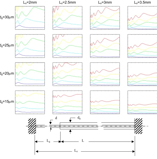
Figure 2.7 shows the frequency plots for a range of total lengths and end
diameters for the same geometry as in Figure 2.6. The axes, which are the
same as in Figure 2.6, are not displayed here due to space limitations. When
the plots are displayed collectively in this manner, trends can be identified.
Firstly, increasing the overall length, Lo, has the effect of reducing the relative
stiffness of the wire, giving a noticeable reduction in the magnitudes of the
natural frequencies, moving from the left to the right in a row. Secondly,
decreasing the end diameter, dg, has the effect of decreasing the relative
stiffness, again clearly visible moving down in a column. The bottom row, for
dg of 15 µm, has no region where the first and second natural frequencies are
particularly close. Here, closeness is assumed to be within 10%. Therefore,
it is expected that these geometries would be susceptible to large amplitude
vibration. The row corresponding to a dg of 20 µm shows promising
geometries for Lg/L of between 1 and 2, for overall lengths of 3 and 3.5 mm.
Figure 2.7. Frequency plots for fixed-fixed beam type, Figure 2.5(a), repeated here for clarity. The vertical and horizontal axes of each subplot are the same as in Figure 2.6. Each column has a different total wire length, and each row has a different end diameter, as shown.
Similar frequency plots can be generated for the other nine beam types
presented in Figure 2.5. Here, Figures 2.8 to 2.16 correspond to beam types
(b) to (j), respectively. The frequency plots in Figure 2.8 show regions were
the third and fourth modes are pushed close together, such as for Lg/L of 1
dg=25µm
dg=20µm
dg=15µm
dg=30µm
Lo=3mm Lo=3.5mm
Lo=2mm Lo=2.5mm
d dg
L Lg
Lo=3mm Lo=3.5mm
Lo=2mm Lo=2.5mm
dg=25µm
dg=20µm
dg=15µm
dg=30µm
dg d
L Lg
with Lo=2.5 mm and dg=30 µm, but not the first and second. Therefore, beam
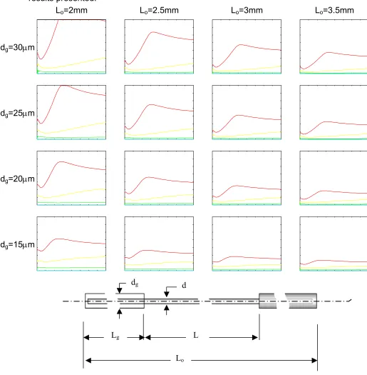
type (b) is not a promising geometry. The frequency plots in Figure 2.9 show
more promising results towards the upper right hand corner, and therefore, a
stepped beam of type (c) would benefit from having a large diameter ratio and
Figure 2.9. Frequency plots for beam type (c) as shown in Figure 2.5(c).
Figure 2.10 is the first of the free-free geometries. For these free-free cases,
the first two natural frequencies calculated by the solution of the eigenvalue
problem are zero, corresponding to rigid body modes where the beam is
translating or rotating about an axis. This is simply the result of having no
boundary constraints and can safely be excluded. Hence, for these free-free
dg d
L Lg
Lo
Lo=3mm Lo=3.5mm
Lo=2mm Lo=2.5mm
dg=25µm
dg=20µm
dg=15µm
cases, the first natural bending frequency, corresponding to the third
eigenvalue, is shown in green. For this geometry, there are no promising
results presented.
d dg
L Lg
Lo
Lo=3mm Lo=3.5mm
Lo=2mm Lo=2.5mm
dg=25µm
dg=20µm
dg=15µm
dg d
L Lg
Lo
beam having this stepped geometry would be less susceptible to large
amplitude vibration. Modifying the overall length gives no apparent benefit
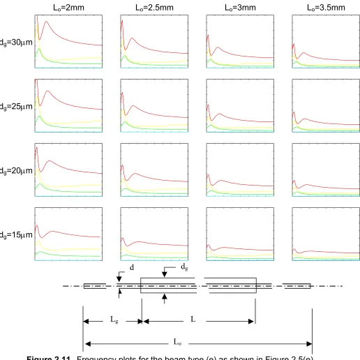
here. In Figure 2.12, beam type (f), also shows some promising geometries,
this time in the top right hand corner for Lg/L of around 3.5, suggesting that a
larger overall length along with a large diameter ratio is expected to be
beneficial.
Figure 2.11. Frequency plots for the beam type (e) as shown in Figure 2.5(e).
Lo=3mm Lo=3.5mm
Lo=2mm Lo=2.5mm
dg=25µm
dg=20µm
dg=15µm
Figure 2.12. Frequency plots for beam type (f) from Figure 2.5(f).
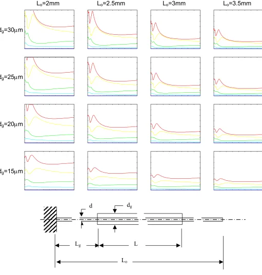
Figure 2.13, the first of the fixed-free geometries, shows no regions where the
first and second natural frequencies are close. Similarly, for Figures 2.14 and
dg d
L Lg
Lo
Lo=3mm Lo=3.5mm
Lo=2mm Lo=2.5mm
dg=25µm
dg=20µm
dg=15µm
frequency plots corresponding to dg values of 30 and 25 µm. This trend
suggests that large step changes in the cross sectional diameters will be of
benefit, for any overall length.
Figure 2.13. Frequency plots for beam type (g) in Figure 2.5(g).
d dg
L Lg
Lo
Lo=3mm Lo=3.5mm
Lo=2mm Lo=2.5mm
dg=25µm
dg=20µm
dg=15µm
Figure 2.14. Frequency plots for beam type (h) as shown in Figure 2.5(h).
dg d
L Lg
Lo
Lo=3mm Lo=3.5mm
Lo=2mm Lo=2.5mm
dg=25µm
dg=20µm
dg=15µm
Figure 2.15. Frequency plots for beam type (i) as shown in Figure 2.5(j).
dg d
L Lg
Lo
Lo=3mm Lo=3.5mm
Lo=2mm Lo=2.5mm
dg=25µm
dg=20µm
dg=15µm
Figure 2.16. Frequency plots for beam type (j) as shown in Figure 2.5(j).
d dg
L Lg
Lo
Lo=3mm Lo=3.5mm
Lo=2mm Lo=2.5mm
dg=25µm
dg=20µm
dg=15µm
Examination of Figures 2.7 to 2.16 reveals similarities in the frequency
patterns. In any of these figures, moving down in a column seems to repeat
the characteristic shapes of the natural frequency curves, only to ‘push’ them
down to lower values. On the other hand, moving from left to right in a row,
seems to both ‘lower’ the curves and ‘zoom out’ to present a wider view.
These similarities lead to the search for scaling parameters. The similarities,
along with attempts to establish scaling parameters, are discussed in the next
section. Scaling parameters would reduce the need to generate so many
2.3 Discussion of Scaling in Frequency Plots
The following discussion is based on fixed-fixed beams, only. However, it
also applies to the other two boundary conditions. Hence, taking beam (a) of
Figure 2.5 as an example, Figure 2.7 shows a selection of frequency against
Lg/L plots for different hot-wire probe geometries. The individual plots in
Figure 2.7 are arranged in such a way that each plot represents a small
change in parameters from those of its neighbours. The plots in the top left
and bottom right do not, at first glance, appear to be similar. However, by
observing the plots that exist in between, similarities can be established.
Figure 2.17 presents a similar case to those given in Figure 2.7 with an end
diameter of 35µm and total length of 3.5mm. The first trend of interest is the
way particular natural frequencies converge, for example the blue,
corresponding to fn1, and cyan, corresponding to fn2, lines at Lg/L=0.75, and
then diverge again as Lg/L increases. This trend is also clearly observed for
all other combinations of neighbouring natural frequencies, such as fn3 and fn4
Figure 2.17. Frequency versus Lg/L plot for a wire having dg=35µm and total
length, Lo=3.5mm.
Another point of interest is the location of Lg/L=0.5, in relation to the fn2 (cyan)
line. As the fn1 (blue) line approaches the fn2 (cyan) line around Lg/L=0.5, the
fn3 (green) line separates. It appears that only two natural frequency lines can
be in close proximity at any given time. When a third natural frequency
approaches to the earlier two, from below, the higher of the earlier two seems
to separate as the value of Lg/L increases. This trend is also present at other
locations, such as for Lg/L=1.25 for the third, fourth and fifth natural
frequencies.
0 0.5 1 1.5 2 2.5 3 3.5 4 Lg/L
70
60
50
40
30
20
10
0
f [kHz]
fn1 (Blue)
fn2 (Cyan)
The third point of interest is the apparent grouping of natural frequencies,
within the frequency range of interest. The first and second natural
frequencies have only one peak, whereas the third and fourth have two
peaks. Following with this pattern, the fifth and sixth (not shown here) have
three peaks. This trend continues for higher modes.
Each of the frequency plots shown in Figure 2.7 exhibit these discussed
trends. Some of the plots, particularly those with small end diameters, appear
to be stretched versions where the clarity of the trends is ‘diluted’. The
existence of such clear trends has led to the search for scaling parameters. A
group of non-dimensionalised parameters to scale the plots would negate the
need for hundreds of trial cases to be explored. Rather, one frequency plot
would ideally show the entire spectrum of possible results. The search for
non-dimensionality has yielded only two partially successful mapping
2.3.1 Scaling Using Mass
The first successful scaling technique relates to the equivalent mass of each
particular geometry. Two frequency plots can be generated where the
geometries have identical end conditions and material properties except for
density. Then, the first can be scaled into the second by the square root of
the ratio of the two densities.
1 2 2 1
ρ ρ ω
ω = ×
where ω1 and ω2, andρ1 and ρ2, are the first natural frequencies and densities
of the first and second geometry, respectively, and ρ1 and ρ2 are the densities
of the two geometries. The origin of this relationship is from the solution of
the natural frequencies of uniform cross sectioned standard Euler-Bernoulli
beams [2]:
( )
2 4ρAL EI
βL
ω=
where: ω is the natural frequency,
β is a constant relating to the boundary conditions and the
particular mode of interest,
E is the Young’s modulus of the beam,
I is the moment of inertia of the beam,
ρ is the density of the beam,
A is the cross sectional area, and
L is the length of the beam.
The usefulness of this scaling is that by varying the density, the absolute
values of the frequencies can be changed rather than the relative
distributions, provided that densities corresponding to real materials are
chosen. Since both geometries here have the same E, I, A, L and β, the
relationship in Equation 2.2 reduces to Equation 2.1. It follows that the other
parameters in Equation2.2 can be scaled in the same manner.
4 1 1 1 2 2 4 2 2 2 1 1 2 1 4 2 2 2 2 2 4 1 1 1 1 1 2 1 L A ρ I E L A ρ I E ω ω L A ρ I E L A ρ I E ω ω = =
Hence, after generating one frequency plot, another can be generated for a
new geometry with identical end conditions using equation 2.3. The limitation
of this scaling technique is that all sections of the beam must be uniform for
the parameter analysed. That is, each section of the stepped beam needs to
have the same material properties. For example, a steel beam can be
geometry 1, and an aluminium beam could be geometry 2. Geometry 2
cannot have aluminium end sections with, for instance, a tungsten middle
section.
2.3.2 Scaling Using Individual Standard Beam Equations
Perhaps the most interesting of all trends in the frequency plots presented in
Figure 2.7, is seen clearly only by modifying Figure 2.17. Rather than
different colours being used for each of the natural frequency lines shown in
Figure 2.17, Figure 2.18 has all the lines drawn in the same colour. Now, a
pattern can be recognised in the way that the ‘first peak’ of each line is
positioned. A line, possibly a hyperbola, can be superimposed onto the plot
so that it covers the ‘first negative gradient portion’ of all five of the natural
frequency lines. A similar line can be drawn covering the ‘second negative
gradient portions’ of the third, fourth and fifth natural frequency lines. A third
0 0.5 1 1.5 2 2.5 3 3.5 4 Lg/L
Figure 2.18. Frequency versus Lg/L plot for the same hot-wire shown in Figure
2.17 having dg=35µm and total length, Lo=3.5mm. Plotted here
using one colour for all the frequency lines. 70
60
50
40
30
20
10
0 f
line can represent the third negative gradient portion of the fifth natural
frequency line.
More lines can be drawn, this time possibly of parabolic type, linking the ‘first
positive gradient portion’ of the first natural frequency with the ‘second
positive gradient’ of the third natural frequency and the ‘third positive gradient’
of the fifth natural frequency line. Similarly, the remaining positive gradient
portions of each of the other frequency lines can also be linked with parabolic
shaped patterns, such as the ‘first positive gradient’ of the second natural
frequency with the ‘second positive gradient’ of the fourth natural frequency
lines.
The hyperbolic and parabolic trends in Figure 2.17 can be mapped by using
the solutions of ‘equivalent’ uniform beams. In order to follow this process,
an analysis was conducted on each section of the stepped beam separately,
rather than on the entire geometry as a whole. As shown in Figure 2.19, the
stepped beam was divided into two uniform cantilevered beams, and one
uniform fixed-fixed beam, each corresponding to the sections of the original
The natural frequencies of each of the individual sections, shown in Figure
2.19, were then calculated, from the closed form exact solutions [2], and
plotted in Figure 2.20. Firstly, for the uniform cantilevered beam in Figure
2.20(a), a hyperbolic trend is observed. Moving from the left to the right on
the horizontal axis, as Lg/L increases, the length of the uniform section
increases such that the beam becomes more flexible, and hence, its natural
frequency decreases. Conversely, in Figure 2.20(b) the plot for the uniform
fixed-fixed beam exhibits parabolic frequency trends. Moving from the left to
right on the graph corresponds to a decrease in the length of the section, so
that it becomes more rigid, and its natural frequency increases.
70
60
50
40
30
20
10
0
Figure 2.20. Frequency distribution plots for the individual uniform beam geometries shown, plotted on the same scale as in Figure 2.18.
f [kHz]
0 0.5 1 1.5 2 2.5 3 3.5 4
Lg/L
Lg
0 0.5 1 1.5 2 2.5 3 3.5 4
Lg/L
Lg
Figure 2.21 shows the individual section frequencies plotted over the
frequencies of the original stepped beam. The red line, corresponding to the
natural frequencies of the stepped geometry, closely follows the blue and
green lines of the middle and end sections, respectively. For example, the
second mode (red) involves the 1st blue curve and the 1st green curve. The third mode (red) involves the 1st and 3rd blue curves and the 1st and 2nd green
curves. Hence, the natural frequency plots for the stepped geometry can be
mapped using two standard uniform beam equations, rather than having to go
through the lengthy finite elements solutions.
0 0.5 1 1.5 2 2.5 3 3.5 4 L /L
70
60
50
40
30
20
10
0
f [kHz]
Blue
Green
The correlation between the natural frequency separations of the stepped
geometry and those of the individual sections is suspected to be only valid for
significant step changes in section diameters, as seen previously in Figure
2.7. The middle section of the geometry needs to be able to vibrate largely on
its own, as if it were mounted between two fixed ends.
There is a clear mismatch between the red lines and the interchange between
the blue and green lines in Figure 2.21. The red line intersects with the blue
line, and they have similar slopes, then it asymptotes towards the green line.
The degree of mismatch is dependent on the magnitude of the step change
between the thick and thin cross sections of the stepped beam. Investigations
have shown that as the step change decreases, so does the correlation
between the frequencies. As a guide, if the step change between the two
sections is at least 5 times, then, a reasonable match is observed. If a larger
step change is practicable, of around 10 times, then a closer match is
expected.
The procedure outlined in this section can be used to eliminate the number of
trial searches required. When a promising curve is found, the frequency
2.4 Conclusions
In this chapter, a novel technique has been introduced for the control of
transverse vibrations of slender beams. The technique relies on modifying
the structure slightly to achieve close first and second natural frequencies.
When the first and second natural frequencies are close, the beam attempts
to have both mode shapes exist simultaneously. The resulting mode shape is
a combination of the first and second mode shapes. This combined mode
shape is ‘unbalanced’ as there are two mode shapes equally possible for the
same frequency. This particular situation restricts the beam’s vibration from
building to resonance in any one particular mode. A numerical procedure is
outlined here for the general case of a fixed-fixed beam geometry. Scaling
and trends of the numerical results are discussed. The next three chapters
Chapter 3
SENSING WIRE VIBRATION OF HOT-WIRE PROBES
3.1 Introduction
Hot-wire anemometry is a powerful and practical technique for measuring
mean and fluctuating fluid velocities and temperatures. It is relatively
inexpensive and easy to use for research, teaching and industrial
applications. The sensing component of a hot-wire probe is a thin wire,
typically in the order of 2 to 6 micrometers in diameter and about 3 millimetres
in length. In Figure 3.1 the sensing wire mounted between two prongs is
shown.
For traditional isothermal applications, the sensing wire is kept at a constant
temperature of about 300o C during measurements, when used in the constant temperature anemometry (CTA) mode. The cooling effect of the
(a) (b) (c)
(Dimensions are shown in mm)
Figure 3.1. Showing (a) hot-wire probe in entirety, (b) hot wire alone [11] and
(c) electron microscope photograph of wire and prong connection [12].
As shown in Figure 3.2, the hot wire probe forms one resistor in a
Wheatstone bridge. Two fixed resistors (R1 and R2) and an adjustable
resistor (R3) complete the Wheatstone bridge. Oncoming fluid velocity cools
the sensor and causes bridge unbalance. A differential feedback amplifier
senses the bridge unbalance and adds current to maintain the temperature of
the sensor [13]. Since the feedback amplifier responds rapidly, the sensor
temperature remains virtually constant as the velocity changes [14]. The
voltage change required to maintain the constant sensor temperature is
interpreted as the velocity of the oncoming fluid through a calibration
Figure 3.2. The block diagram of a constant temperature anemometer [13].
The underlying assumption of the interpretation discussed in the preceding
paragraph is that the wire is stationary, and the velocity of the flow ‘relative’ to
the wire can be assumed to be the ‘absolute’ velocity. However, due to its flexibility, the hot-wire probe is susceptible to large amplitude resonance
vibrations. As a result of these vibrations, the relative velocity can no longer
represent a close indication of the absolute flow velocity.
A turbulent flow approaching the wire has mean and fluctuating velocity
components. The mean velocity can cause a deflection of the wire, which is
best described as causing a constant sag or curve in the wire. Wires are
manufactured with a pre-tension, which may compensate for this effect. This
curve does not present a significant problem to the accuracy of the
measurements, since it causes no fluctuations in the wire displacement.
However, the fluctuating velocity component of the flow can cause the wire to
Feedback Amplifier
Bridge unbalance sensed here Probe
Anemometer output voltage measured here
R1 R2
resonate. Each velocity fluctuation in the flow has an associated fluctuating
force that leads the wire displacement by a phase angle of 90 degrees at
resonance [2]. On the other hand, the wire velocity always leads the
displacement by 90 degrees. Hence, at resonance, the velocity of the wire is
in phase with the excitation force fluctuations. Therefore, the velocity of the
wire is in phase with the velocity fluctuations in the flow. This presents a
significant problem, if the velocity fluctuations of the wire are comparable in
magnitude to the velocity fluctuations in the flow. It is easy to see that if the
wire has the same amplitude velocity fluctuations as those of the flow velocity,
then there would be no relative velocity between the wire and the flow. Zero
relative velocity is, of course, an unlikely condition. However, the relative
velocity sensed by the probe wire can be somewhat smaller than the absolute
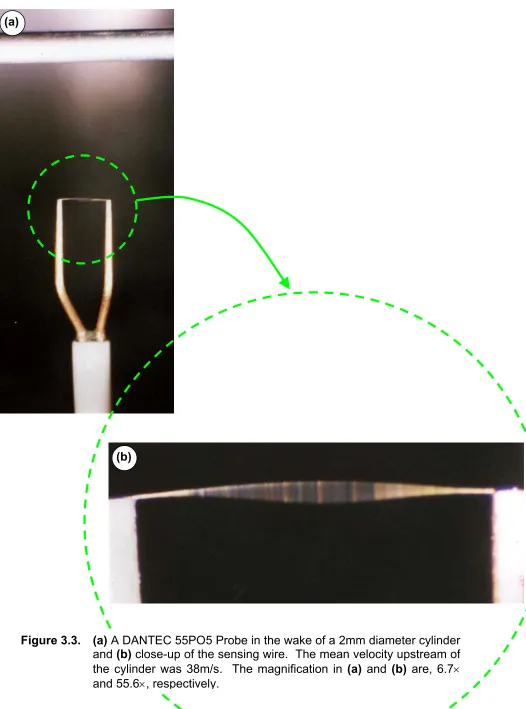
velocity of the flow. In Figure 3.3 (a) a hot-wire probe is shown in the wake of
a cylinder, where the flow is from top to bottom. A close up of the blurry
envelope in Figure 3.3 (b) indicates the stream-wise vibrations possible in
turbulent flow.
In this chapter, the limited works related to the vibration of a hot-wire probe
are reviewed in the next section. In section 3.3, a numerical model is
introduced. The numerical predictions are discussed in Section 3.4. The
scaled-up experimental results and the actual size flow measurements are
Figure 3.3. (a) A DANTEC 55PO5 Probe in the wake of a 2mm diameter cylinder and (b) close-up of the sensing wire. The mean velocity upstream of the cylinder was 38m/s. The magnification in (a) and (b) are, 6.7×
and 55.6×, respectively.
(a)
3.2 Earlier Work
The problem of wire vibration was first observed by Perry et al. [15, 16]. This
work investigated two types of wire vibration, namely, rotational vibration and
skipping (or whirling) of the wire. However, the more predominant case of
stream-wise transverse vibrations had not been investigated in detail before
the work of [8].
This earlier study in reference 8 indicated measurement errors when large
amplitude wire vibrations are expected. It suggested that the filament of a
hot-wire probe can be excited at its first or higher resonance modes. If the
probe wire is excited in the first mode, the resulting vibration velocity is
in-phase with the velocity fluctuations in the flow along the entire wire length as
mentioned earlier. Hence, these in-phase oscillations may reduce the relative
velocity between the wire and the flow, leading to smaller readings than the
true absolute velocity of the flow. Therefore, hot wire dimensions must be
chosen such that the resulting first natural frequency of the wire is larger than
the expected frequency content in the flow.
One way to achieve a high first natural frequency of the wire is to use a short
wire. However, a short wire causes heat conduction loss to the prongs. Heat
The earlier work in [8] investigated the differences in the experimental results
obtained with different probes under the same flow conditions. It showed that
large measurement errors were present for some probes, while others had
more accurate results. For cases when the first natural frequency is within the
frequency range of excitation, the most accurate measurements were
observed when the first and second natural frequencies of the probe wire
were close numerically. This earlier investigation pointed out a limited
number of already existing favourable designs. However, no effort was made
to look at new designs with improved dynamic characteristics. It is this
determination, which forms the basis for this research thesis. The objective
here has been to explore the possibilities of linking the first and second
natural frequencies together to achieve favourable vibration characteristics.
3.3 Numerical Modelling
Application of the technique discussed in Chapter 2 to a hot-wire probe, was
commenced by numerically modelling the particular slender beam of interest.
The geometry of a hot-wire probe sensing wire can be modelled using beam
type (a) from Figure 2.5, which is shown again here in Figure 3.4 for
convenience. In this figure, the middle sensing wire has d and L for diameter
and length, whereas dg, Lg and Lo represent the diameter and the length of the
thicker ends and the total length of the wire, respectively. Boundary
conditions are taken to be built-in where the wire is welded to the prongs. The
electron microscope photograph presented in Figure 3.1 (c), justifies this
boundary condition by clearly showing the welded connections.
Hot-wire probes are manufactured with an intentional pre-tension at room
temperature. The numerical model does not include this pre-tension. The
presence of any wire pre-tension would simply increase all the natural
frequencies by the same scale, rather than making any relative changes. In
d dg
addition, pre-tension may be lost when the wire is heated for flow
measurements.
3.3.1 Numerical Model
Along the length of the wire, 30 standard finite beam elements [2] were used
to approximate the dynamic properties of the model in Figure 3.4. The three
sections of the beam had ten elements each, a sufficient number to give an
accurate representation of the first five mode shapes. The minimum number
required was found to be 6 elements, so 30 is ample. Solution of the resulting
eigenvalue problem in Matlab® [10] provided the first 58 natural frequencies
for the wire, of which the first five were of interest, since the higher modes are
well outside the frequency range of flow excitation.
Dynamic response of the wire to a broadband, random white noise excitation
force was obtained by numerically integrating the system differential
equations of motion using the Newmark-β technique [2]. The white noise was
generated in Matlab® [10] using the built in random number generator, then
scaling the output to the desired frequency by altering the time step. The
frequency content of the excitation force (zero to 50 kHz) was sufficient to
excite up to the fifth mode of the wire. Broadband excitation may be assumed
to be indicative of the forces that a wire experiences when placed in a
turbulent flow. This external force was applied at one node to the right of the
mid-point so as to be able to excite the even numbered modes, which have
nodes at the mid-point. A single node input was chosen rather than a
discussed later. Structural damping of 1% was used in the model. 50,000
steps of integrations were performed with a time step of 10 µs to allow the
root mean square (rms) of the displacement to settle to within 1% of its steady
state value.
One of the existing hot-wire probe geometries, Probe 3 in [8], is investigated
here as the starting geometry. This probe has a total length of 3 mm, a
sensitive length and diameter of 1.18 mm and 5.75 µm, respectively, resulting
in a sensitive length to diameter ratio, L/d, of 205. It has a thick end diameter
of 30 µm. The probe wire has a platinum core plated with tungsten, and its
thicker ends are plated with gold. Previous research showed that Probe 3
was the least susceptible to large amplitude vibrations, and one of the most
accurate for measurements in turbulent flow [19]. The objective here has
3.3.2 Numerical Predictions
The effect of varying the ratio of the length of the end sections to the sensitive
length, Lg/L, is shown in Figure 3.5. From left to right along the horizontal
axis, the ratio of the end length to the sensitive length, Lg/L, increases. This
increase results in a smaller L and larger Lg for a constant Lo of 3 mm. The
ratio of the end length to the total length, Lg/Lo, is also shown as a second
horizontal axis for reference. The vertical axis represents the five resonance
frequencies of the wire corresponding to the five curves given in ascending
order. Figures 3.5(a), 3.5(b) and 3.5(c) correspond to end diameters, dg, of
15µm, 30µm and 45µm, respectively.
The starting geometry of Probe 3 is marked with a vertical dashed line at Lg/L
of 0.77 in Figure 3.5(b). As Lg/L increases from the starting value of 0.77 in
this figure, the first (fn1) and second (fn2) resonance frequencies move closer,
while the third resonance frequency is pushed away. Furthermore, the third
and fourth resonance frequencies also approach one another as Lg/L
increases. As the thick ends increase in length, they become more flexible
and participate more actively in vibrations. It appears that thick ends can
participate a lot more readily in the first two modes as compared to the higher
ones. As a result, increasing Lg/L generally gives smaller fn1 and fn2; while
higher modes can exhibit initial rapid increases before levelling off and then
decreasing gradually. This trend is most clearly observed in Figure 3.5(c),
where dg is 45 µm, whereas Figure 3.5(a) shows only slight changes in the
Figure 3.5. Variation of the first five natural frequencies with L /L for d of (a)
0.5 1 1.5 2 2.5 3 3.5 4
0 10 20 30 40 50 60 70 4 f(kHz) (c) 0 10 20 30 40 50 60 70 4 f(kHz) (b) 0 10 20 30 40 50 60 70 4 f(kHz) (a)
Lg/Lo
Lg/L
The effect of Lg/L decreasing from the starting value of 0.77 in Figure 3.5 (b),
is the relative separation of the resonance frequencies. For Lg/L of
approximately 0.2, all five resonance frequencies become almost equally
spaced. The reason for this trend originates from the effective stiffening of the
ends as they become shorter. Short ends contribute less to the dynamic
response. The response of the sensing wire overwhelms that of the thick
ends, eventually approaching the case of a uniform beam consisting of the
sensing section alone with well-separated natural frequencies.
Eight representative end length to sensitive length ratios (of 0.5, 0.77, 1, 1.13,
1.5, 2, 2.5 and 3) were chosen from Figure 3.5, and the resulting probe wire
models were subjected numerically to a broad band excitation to obtain their
dynamic responses for comparison. The results of this excitation are shown
in Figure 3.6. In Figure 3.6, a value of zero on the horizontal axis represents
the middle of the wire. The vertical axis is the normalised rms of the
displacement amplitude. The vertical axis is normalised by dividing the rms
response of each case by a scaler parameter, which is the rms response of
Probe 3 in the mid span. Probe 3 from reference [8] was previously shown to
be the best existing design. Probe 3 is marked with (o) in Figure 3.6 (b),
having Lg/L of 0.77, with a total length of 3 mm and an end diameter, dg of 30
µm. Hence, any new probe with a normalised rms response smaller than
unity represents a desirable structural improvement. Any normalised
response larger than unity, however, indicates a detrimental effect due to
geometric changes. Clearly, reduction in the end diameter to 15 µm, has a
Beam axis (mm) Normalised
rms response
(a) 3
2
1
(b) 1.5
1
0.5
(c) 1.5
1
0.5
-1.5 -1 -0.5 0 0.5 1 1.5 0
0 0
Figure 3.6. Variation of the normalised rms displacement response for random white noise excitation and for dg of (a) 15 µm, (b) 30 µm and (c) 45 µm.
Figure 3.6(b) shows the reduction in amplitude achievable by altering Lg/L.
The best, lowest amplitude, case is for Lg/L of 3 (@). It is notable, however,
that there is little difference in amplitude between geometries having Lg/L of
between 1.5 (Z) and 3 (@). Figure 3.6(c) shows the rms amplitudes for
probes with an increased end diameter dg of 45 µm. Here, a probe with Lg/L
of 1.5 (Z) has comparable amplitude to that having Lg/L of 1.5 (Z) with dg of
30 µm. However, unlike the case for 30 µm, increasing Lg/L to 3 (@), reduces
the RMS amplitude significantly for 45 µm.
A more concise presentation of this data may be achieved by plotting only the
mid-span rms amplitude for each geometry, as shown in Figure 3.7. Similar
0 .5 1 1 .5 2 2 .5 3
260 174 130 104 87 75 L/d
Normalised rms response in the
mid-span
Figure 3.7. Variation of the peak rms displacement at the mid-span with L /L 3
2
1
0
Lg/L