Article
Parameters identification for inverse option problems
using Markov Chain Monte Carlo methods
Yasushi Ota1,∗ and Yu Jiang2
1 Department of Management, Okayama University of Science, 1-1 Ridaicyou, Okayama City, Okayama
1
2
3
4
5
6
7
8
9
7000005 Japan; [email protected]
2 School of Mathematics, Shanghai University of Finance and Economics, 777 Guoding Rd.,Shanghai,200433,P.
R.China;[email protected]
* Correspondence:[email protected];Tel.:+81-086-256-9805
Abstract:Thispaperinvestigatestheinverseoptionproblems(IOP)intheextendedBlack–Scholes modelarisinginfinancialmarket.Weidentifythevolatilityandthedriftcoefficientfromthemeasured datainfinancialmarketsusingaBayesianinferenceapproach,whichispresentedasanIOPsolution. Theposteriorprobabilitydensityfunctionoftheparametersiscomputedfromthemeasureddata. ThestatisticsoftheunknownparametersareestimatedbyaMarkovChainMonteCarlo(MCMC) algorithm,whichexploitstheposteriorstatespace. TheefficientsamplingstrategyoftheMCMC algorithmenablesustosolveinverseproblemsbytheBayesianinferencetechnique.Ournumerical resultsindicatethattheBayesianinferenceapproachcansimultaneouslyestimatetheunknowntrend andvolatilitycoefficientsfromthemeasureddata.
Keywords:Inverseproblem;Optionpricing;Bayesianinferenceapproach 10
1. Introduction 11
The technique of inverse problems for a partial differential equation of a parabolic type is 12
developed and used in various fields, such as Inverse heat transfer problems(IHTP), Inverse heat 13
conduction problems(IHCP), Inverse option problems(IOP), etc[1,2,4]. 14
In this paper we consider the backward parabolic eauation:
∂u ∂t +
1 2σ(x,t)
2x2∂2u
∂x2+µ(x,t)x ∂u
∂x −ru=0, (x,t)∈(0,∞)×[0,T),
u(x,t)|t=T=Φ(x,T), x∈(0,∞).
(1)
where u(x,t)is the price for a derivative, such as an option, bond, interest rate, futures, foreign 15
exchange, etc. Moreover,xin the underlying asset price,tis the time,σ(x,t)andµ(x,t)are the drift
16
and volatility coefficient of the processx, the interest rateris a nonnegative constant, andKis the 17
strike price andTis the maturity of the underlying asset, andΦ(x,T)is a suitable initial condition. 18
Now, we are interested in the following inverse option problem(IOP): Let the current timet∗be given , 19
and determine simultaneouslyµ(x,t)andσ(x,t)from the observation of datau(x,t∗),x ∈ω, where
20
ωis the interval.
21
IOP in mathematical finance were started by Dupire [8]. He derived the option premiumU(T,K)
as a solutionu(·,·;T,K)to the dual equation of Black-Schoels equation, which isµ=rin (1), with
respect to the strike priceKand maturity T as follows:
∂U ∂T −
1
2σ(T,K)
2K2∂2U
∂K2 +rK ∂U
∂K =0. (2)
If the option price and its derivative can be determined for all possibleTandK, then the local volatility functionσ(T,K)can be directly derived from Eq.(2) as
σ(T,K)2= ∂U
∂T +rK ∂U ∂K
1 2K
2∂2U
∂K2
. (3)
Using this approach, we can deduce the local volatility function from the quoted option prices in the financial market. Bouchouev and Isakov [4], Bouchouev et al. [5], and Ota and Kaji [24], by using a linearization method, considered the following form of the time–independent local volatility function
σ2(K):
1 2σ
2(K) = 1 2σ
2
0+f(K)
where f is a small perturbation of the constant volatilityσ0. Moreover, Mitsuhiro and Ota [23], Korolev 22
et al. [17] and Doi and Ota [9] used the extended Black–Scholes equation (1) and then reconstructed 23
the trend function by linearization method. The above studies provided point estimates of unknown 24
parameters by exact determination or least squares optimization, without rigorously examining and 25
considering the measurement errors in the inverse solutions. In [25] we reconstruct the parameters not 26
by linearizing the inverse problems but by applying Bayesian inference to IOP. 27
In this paper, we investigate the Binary Option Problem, which has an initial conditionΦ(x,T) =
H(x−K)in (1), whereHis the Heviside function, that is,
H(x−K) =
(
1 x≥K 0 x<K.
And we attempt a parameter reconstruction by a statistical method that simultaneously estimates the 28
unknown trend and volatility coefficients from the measured data. 29
Bayesian inference approach solves an inverse problem by formulating a complete probabilistic 30
description of the unknowns and uncertainties from the given measured data (see [16]). Incorporating 31
the likelihood function with a prior distribution, the Bayesian inference method provides the posterior 32
probability density function (PPDF). Owing to the recent developments in Bayesian inference work, 33
including Bayesian inference approach by efficient sampling methods such as Markov Chain Monte 34
Carlo (MCMC), we can apply the Bayesian inference technique to inverse problems in remote sensing 35
[11], seismic inversion [21], heat conduction problems [29], [30] and various other real–world problems. 36
Moreover, several prior publications such as [6,14,15,27,28] are related to option pricing based on 37
Bayesian inference. In those publications, the option prices are usually computed by using the 38
analytical solution (or so-called Black-Scholes formula) or applying of Monte Carlo simulation of 39
original stochastic differential equation under an assumption which the volatility is constant. 40
This paper is divided into five parts. Our inverse problem is mathematically formulated in Section 41
2. Section 3 outlines the general Bayesian framework for solving inverse problems and discusses the 42
numerical exploration of the posterior state space by the MCMC method. In Section 4, we discretize 43
our inverse problem and reconstruct the parameters by a numerical algorithm. We then discuss various 44
2. Mathematical formulation of IOP 46
In this paper, we consider that the volatility is a constant (σ(x,t)≡σ0)and the initial condition is a step function in (1):
∂u ∂t +
1 2σ
2 0x2
∂2u
∂x2 +µ(x,t)x ∂u
∂x −ru=0 (x,t)∈(0,∞)×[0,T),
u(x,t)|t=T=H(x−K) x∈(0,∞).
(4)
First, we check an idea of Dupire[8] and derive the partial differential equation dual to (4). 47
We set
G(x,t;K,T) =−∂u(x,t;K,T)
∂K (5)
and thenG(S,t;K,T)satisfies the differential equation (4), and
G(x,T;K,T) =δ(x−K). (6)
According to Friedman[10],G(x,t;K,T)satisfies for fixed(x,t)as a function of(K,T)the following differential equation and initial condition:
∂G ∂T −
1 2
∂2 ∂K2(σ
2 0K2G) +
∂
∂K(µ(K,T)KG) +rG=0 (x,t)∈(0,∞)×[0,T),
G(x,t;K,t)|t=T =δ(x−K) x∈(0,∞).
(7)
Then, we use the definition ofG(S,T;K,T), and integrate the equation (7) fromKto∞. The third term 48
in the left-hand side can be integrated by parts as follows 49
Z ∞
K
∂
∂ξ(µ(ξ,T)ξG)dξ=µ(K,T)K ∂u ∂K
where we have used the following behaviour at infinity
u,K∂u
∂K,K
2∂2u
∂K2 →0 as K→∞
Consequentry, we can obtain the following dual equation foru(·;K,T)
∂u ∂T −
1 2σ0K
2∂2u
∂K2 −(σ0−µ(K,T))K ∂u
∂K+ru=0. (8)
Now, the substitution
y=logK
x, τ=T−t,
µ(y) =µ(K,T), U(y,τ) =u(x,t;K,T)
transforms the equation and the initial condition (4) into
∂U ∂τ −
σ02
2
∂2U ∂y2 −
σ2 0
2 −µ(y) ∂U
∂y +rU=0 (y,τ)∈R×(0,τ
∗),
U(y, 0) =H(−y) y∈R,
(9)
whereτ∗=T−t∗andt∗is the current time.
Then, we consider the following problem IOP: 51
ProblemIf we give the data U∗(x):=U(y,τ∗)onωatτ=τ∗=T−t∗then identifyσ0andµ(y)satisfying
52 (9) 53
However, due to the nonlinearity of this inverse problem, the uniqueness and existence of its 54
solution are hard to prove. In this paper we attempts to reconstruct the parameters by a statistical 55
method simultaneously estimatesµ(y)andσ0from the measured dataU∗(y). 56
Let us definem−dimensional vectorsY,F(θ)andεas follows:
57
{Y}j = U∗(yj) =U(τ∗,yj; ¯θ)(1+εj)
{F(θ)}j = U(τ∗,yj;θ)
{ε}j = εj
whereyj(j = 1,· · ·,m)are the measurement points atτ∗,U(τ∗,yj;θ)solves the Cauchy problem
(9) for the unknown parametersθandεjis the uncertainty (noise) in the market, assumed as white
Gaussian noise with a known standard deviationΣε. We then seek the parameters ¯θ, which assumedly
represent the true value ofθ, such that
Y=F(θ) +ε. (10)
3. Bayesian inference approach to IOP 58
The Bayesian inference approach is now widely used with great successes for solving a variety of inverse problem (see for example [16]). The solution of the Bayesian inference approach is estimated not as single-valued, but as the posterior conditional mean (CM)
θCM:= Z
θf(θ|Y)dθ, (11)
of the unknown parametersθgiven the measured dataY. Here, according to the Bayes’ theorem, the
posterior probability density function (PPDF) is defined as follows:
f(θ|Y) = f(Y|θ)f(θ)
f(Y) . (12)
i.e. the posterior probability of a hypothesis is proportional to the product of its likelihood and its prior probability. The likelihood function f(Y|θ)is then given as
f(Y|θ) =exp
−(Y−F(θ))
T(Y−F(
θ))
2Σ2 ε
. (13)
In some case, since we don’t know much about a prior density function(θ), it is simply assumed as
59
f(θ) =U[−θ0,θ0], whereθ0is a sufficiently large positive constant. Thus, the PPDF of the parametersθ
60
is the same as the likelihood function. 61
3.1. MCMC methods 62
It is hard to know the explicit form of f(θ|Y) in (11), Markov chain Monte Carlo (MCMC)
algorithm given in Robert and Casella [26] can be applied to obtain a set of samplesθk(k=1,· · ·,K)
and these independent samples can approach the distribution f(θ|Y). Also the posterior conditional
mean comes to
θCM≈ 1 K
K
∑
k=1θk.
In this paper, we employs a typical MCMC algorithm called the Metropolis–Hastings (M–H) 64
algorithm (see Metropolis et al. [22]; Hastings [12]).M–H Algorithmgiven below builds its Markov 65
chain by accepting or rejecting samples extracted from a proposed distribution.M–H Algorithmis 66
generally used in Bayesian inference approach (cf. [16]). 67
M–H Algorithm 68
• Step1: Generate θ0 ∼ q(·|θk) = N(θk,γ2) (the normal distribution) with a given stander
69
derivationγ>0 for givenθk.
70
• Step2: Calculate the acceptance rateα(θ0,θk) =min{1,f(θ0|Y)/f(θk|Y)}.
71
• Step3: Updateθkasθk+1=θ0with probabilityα(θ0,θk)but otherwise setθk+1=θkand re-sample
72
from 1. 73
While running this M–H algorithm, we can find, by given any initial guessθ0, the samples will come to a stable Markov chain after a burn-in timek∗. In other word, unlike common Newton–type iterative regularization methods (for example, the Levenberg–Marquardt algorithm), the MCMC algorithm does not highly depend on the initial guess and the mean value
θCM≈ 1 K−k∗
K
∑
k=k∗+1θk,
always reaches the global minimum after a sufficiently long sampling time. 74
4. Numerical examples 75
In this section, we generate numerically an exact artificial data set F(θ) and let (10) be the
numerical data. In the rest of this paper, we assume the trendµ(y)has the form:
µ(y) =r+αy+βy2+γy3, (14)
whereα,β,γare the unknown constant. We also assume the measurement dataYhas the form:
Y=F(θ) +ε, (15)
where random errorεcontains both the random measurement error and the numerical error. By
76
reconstructing the parameters by the M–H method, we simultaneously estimateα,β,γandσ0from the 77
measured dataYin (15). 78
4.1. Direct problems 79
In this section, we assume r = 0 and solve the direct problem for (9) by the numerical 80
Crank–Nicholson scheme: 81
ajUi+1,j+1+ (1+b)Ui+1,j+cjUi+1,j−1
=−ajUi,j+1+ (1−b)Ui,j−cjUi,j−1, (16)
whereUi,j =U(ti,yj), and
aj=− ∆
τ
4(∆y)2
σ02+∆y
1 2σ
2
0−(αy+βy2+γy3)
,
b= ∆τ
2(∆y)2,
cj=− ∆
τ
4(∆y)2
σ02−∆y
1
2σ 2
0−(αy+βy2+γy3)
Here, we took a uniform grid 82
˜
ω={(τi,yj):τi ∈(0,τ∗), yj∈ I1.5= (−1.5, 1.5),
i=1, 2,· · ·, 400,j=1, 2,· · ·, 100}
with artificial zero Dirichlet boundary conditions aty=−1.5 and 1.5, such asUi,1=1 andUi,100=0, 83
and∆τ=τi+1−τi =0.001, ∆y=yj+1−yj= 331.
84
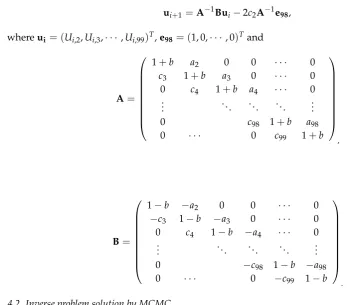
Then (9) can be given in the matrix form:
ui+1=A−1Bui−2c2A−1e98, (17)
whereui= (Ui,2,Ui,3,· · ·,Ui,99)T,e98= (1, 0,· · ·, 0)Tand
A=
1+b a2 0 0 · · · 0 c3 1+b a3 0 · · · 0 0 c4 1+b a4 · · · 0 ..
. . .. . .. . .. ...
0 c98 1+b a98
0 · · · 0 c99 1+b , 85 B=
1−b −a2 0 0 · · · 0 −c3 1−b −a3 0 · · · 0 0 c4 1−b −a4 · · · 0 ..
. . .. . .. . .. ...
0 −c98 1−b −a98
0 · · · 0 −c99 1−b .
4.2. Inverse problem solution by MCMC 86
Table 1 shows the true values and parameter settings in M–H Algorithm. 87
Table 1.Parameter setting in M–H Algorithm.
Parameters α β γ σ0
True value 1 1 1 1
σθ 0.01 0.01 0.01 0.01
In the following examples, the relative noise in all the observationsYis assumed as 1% and 5%, and the prior distributionf(θ)of unknowns is(α,β,γ,σ0) =1. That is, we can say
fprior(θ) =1[αmin,αmax](α)·1[βmin,βmax](β)·1[γmin,γmax](γ)·1[σmin
0 ,σ0max](σ0)
and the intervals[αmin,αmax],[βmin,βmax],[γmin,γmax]and[σ0min,σ0max]are large enough so that all
(α,β,γ,σ0)’s appearing in the Markov chain fall into these intervals. Here, we set the the indicator function as
1A(a) =
(
General uniform distributions can be used forf(θ)if we use the prior-reversible proposal that satisfies
88
f(θ)q(θ0|θ) = f(θ0)q(θ|θ0)(see for example [13]). On the other hand, if we choosef(θ)as a Gaussian
89
distribution, this will turn out to be the Tikhonov regularization term in the cost function. 90
For comparison, we particularly consider the Levenberg-Marquardt algorithm [18,20]. That is, the recovery ofθ= (α,β,γ,σ0)Tis computed by the iteration given by
θk+1=θk+
h
F0(θk)TF0(θk) +λI
i−1
F0(θk)T(U−F(θk)), (18)
where F0(a) is the Jacobian matrix and the parameter λ is nonnegative. This algorithm can be
91
implemented for example by an inner embedded programlsqcurvefitin MATLAB 2018a. 92
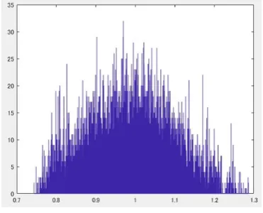
Example 1: In this example, we set the initial guess of(α,β,γ,σ0)as(0, 0, 0, 0). Figure1, Figure3, 93
Figure5, Figure7are the trace plots of the chain for(α,β,γ,σ0), respectively. We can see that the chain 94
mixes well. Moreover recovered results for the posterior probability density function are presented 95
in Figure2, Figure4, Figure6, Figure8, and Table2. From these results the recovery of(α,β,γ,σ0) 96
represents an excellent approximation of the ture value(1, 1, 1, 1). Here, “Mean value(with 1% noise) 97
and Mean value(with 5% noise)” in Table2are the average of the value of the iteration time 30000 98
after burn-in time 5000. For comparison, the converged recovery of (α,β,γ,σ0) obtained by the 99
Levenberg–Marquardt algorithm for the measured data with 5% noise is also provided in Table2. 100
Figure 1.The trace plot ofα
Figure 2.The posterior density forα
with 1% noise added into the data
Figure 3.The trace plot ofβ Figure 4.The posterior density forβ
Figure 5.The trace plot ofγ Figure 6.
The posterior density forγ
with 1% noise added into the data
Figure 7.The trace plot ofσ0
Figure 8.The posterior density forσ0
Table 2.Recovery results of(α,β,γ,σ0).
Parameters α β γ σ0
Initial guess 0 0 0 0
Mean value(with 1%noise) 0.9887 0.9888 1.0022 1.0030
Result of LM 0.9895 0.9936 1.0054 1.0031
Mean value(with 5% noise) 1.0556 0.9881 0.9473 0.9912
Result of LM 1.0662 0.9991 0.9504 0.9894
True value 1 1 1 1
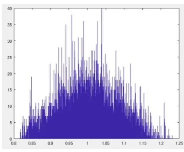
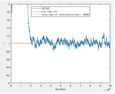
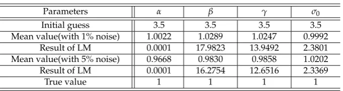
Example 2: 101
In this example, the initial guess of(α,β,γ,σ0)was set(3.5, 3.5, 3.5, 3.5)to the value far from 102
the true value(1, 1, 1, 1). The evolutions of the MCMC sampledα,β,γandσ0are shown in Figure 103
9, Figure11, Figure13, Figure15respectively, and we can see that the chain mixes well. Moreover 104
recovered results for the posterior probability density function are presented in Figure10, Figure12, 105
Figure14, Figure16, and Table3. From these results the recovery of(α,β,γ,σ0)represents an excellent 106
approximation of the ture value(1, 1, 1, 1). The divergent recovery of(α,β,γ,σ0) obtained by the 107
Levenberg–Marquardt algorithm for the measured data with 5% noise is also shown in Table3. 108
Figure 9.The trace plot ofα Figure 10.The posterior density forα
with 1% noise added into the data
Figure 11.The trace plot ofβ Figure 12.The posterior density forβ
Figure 13.The trace plot ofγ
Figure 14.The posterior density forγ
with 1% noise added into the data
Figure 15.The trace plot ofσ0 Figure 16.The posterior density forσ0
Table 3.Recovery results of(α,β,γ,σ0).
Parameters α β γ σ0
Initial guess 3.5 3.5 3.5 3.5
Mean value(with 1% noise) 1.0022 1.0289 1.0247 0.9992 Result of LM 0.0001 17.9823 13.9492 2.3801 Mean value(with 5% noise) 0.9668 0.9830 0.9858 1.0202 Result of LM 0.0001 16.2754 12.6516 2.3369
True value 1 1 1 1
In the case of the initial guess(0, 0, 0, 0), from the results of the MCMC samples in Figure1, 109
Figure3, Figure5, Figure7and the posterior condition mean values are presented in Table2, we can 110
see that we succeeded in recovering parameters. And, in the case of the initial guess(3.5, 3.5, 3.5, 3.5)
111
likewise, from the results of the MCMC samples in Figure9, Figure11, Figure13, Figure15and the 112
posterior condition mean values are presented in Table3, we can see that we succeeded in recovering 113
parameters. 114
On the other hand, in the case of the initial guess (0, 0, 0, 0), the recoveries obtained by the 115
Levenberg–Marquardt algorithm in Table2succeeded as the case of MCMC algorithm. However, 116
in the case of the initial guess(3.5, 3.5, 3.5, 3.5), we could not obtain the results of the recovering 117
parameters by the Levenberg–Marquardt algorithm in Table3. From these results we observe that 118
parameters are more sensitive to initial values than MCMC algorithm and hence it is less easily 119
recovered. 120
5. Conclusions 121
In this study, we have established the method of simultaneous estimation of the unknown drift and 122
volatility coefficients from the measured data, by using a Bayesian inference approach(MCMC-MH) 123
based on a partial differential equation of parabolic type. In particular, we took into account an 124
application to real financial markets and dealt with the case with Heaviside function as the initial 125
condition, so-called binary option. In the instantaneous estimation of trend and volatility coefficients, 126
we assumed that the volatility coefficient is a constant and the trend coefficient is a cubic function with 127
three unknown parameters. The posterior distributions of the unknown trend and volatility coefficients 128
were recovered from the measured data by modeling the measurement errors as Gaussian random 129
variables. The posterior state space was explored by the MCMC–M–H method. As confirmed in the 130
numerical results, the Bayesian inference approach(the MCMC algorithm) simultaneously estimated 131
the unknown trend and volatility coefficients from the measured data than the Levenberg–Marquardt 132
algorithm. 133
There are still several problems we have to settle. First, from the form of our model it is expected 134
that we will be able to apply the results of this study to problems of term structure models for an 135
interest rate. Moreover we will try to identify parameters of another financial model, for instance, such 136
as the model including the dividend yield. Next, we will develop mathematical results (for instance, 137
the uniqueness, stability, and existence) of IOP and extend our approach to two–dimensional cases. 138
Finally, we have to study how to apply our results to the real financial market, and repeat tests. 139
Author Contributions:Investigation, Ota Y. ; Methodology, Ota Y. and Jiang Y. ; Software , Ota Y. (MCMC) and 140
Jiang Y. (MCMC, LM) ; Validation and Writing–original draft, Ota Y. 141
Funding:The first author would like to acknowledge the supports from JSPS Grant-in-Aid for Scientific Research 142
(C) 18K03439. The second author was supported by National Natural Science Foundation of China (No. 11771270). 143
Acknowledgments:In this section you can acknowledge any support given which is not covered by the author 144
contribution or funding sections. This may include administrative and technical support, or donations in kind 145
(e.g., materials used for experiments). 146
References 148
1. Alifanov M. O. 1997Inverse Heat Transfer Problems, International Series in Heat and Mass Transfer,Springer 149
Verlag. 150
2. Beck V. J., Blackwell B. and Clair Jr. C. R. 1985Inverse Heat Conduction: Ill-Posed Problems,Wiley-Interscience. 151
3. Black F. and Scholes M. 1973The pricing of options and corporate liabilities, Journal of Political Economy,81, 152
637-659. 153
4. Bouchouev I. and Isakov V. 1999Uniqueness, stability and numerical methods for the inverse problem that arises in 154
financial markets, Inverse Problems,15, R95-R116. 155
5. Bouchouev I., Isakov V. and Valdivia N. 2002Recovery of volatility coefficient by linearization, Quantitative Finance, 156
Vol2, 257-263. 157
6. Bunnin F. O., Guo Y. and Ren Y. 2002Option pricing under model and parameter uncertainty using predictive 158
densities Statistics and Computing,12(1), 37–44. 159
7. Cui T., Fox C., and O’fSullivan M.J. 2011Bayesian calibration of a large-scale geothermal reservoir model by a new 160
adaptive delayed acceptance Metropolis Hastings algorithm, Water Resource Research,47, W10521. 161
8. Dupire B. 1994Pricing with a smil, Risk,7 18-20. 162
9. Doi S. and Ota Y. 2018Application of microlocal analysis to an inverse problem arising from financial markets Inverse 163
Problems.34, N11. 164
10. Friedman A. 1983Partial Differential Equations of Parabolic Type,(Englewood Cliffs, N.J: Prentice-Hall). 165
11. Haario H., Laine M., Lehtinen M., Saksman E. and Tamminen J. 2004Markov chain Monte Carlo methods for high 166
dimensional inversion in remote sensing, Journal of the Royal Statistical Society: Series B (Statistical Methodology),66, 167
591-608. 168
12. Hastings, W. 1970Monte Carlo sampling methods using Markov chains and their application, Biometrika,57, 97-109. 169
13. Iglesias M. A., Lin K and Stuart A. M. 2014Well-posed Bayesian geometric inverse problems arising in subsurface 170
flow, Inverse Problems,30, 114001. 171
14. Jacquier E. and Jarrow R. 2000Bayesian analysis of contingent claim model error, Journal of Econometrics,94(1-2), 172
145–180. 173
15. Jacquier E. and Polson N. 2010Bayesian methods in finance, Oxford handbook of Bayesian econometrics,439–512 174
(Oxford University Press). 175
16. Kaipio J. and Somersalo E. 2005Statistical and Computational Inverse Problems.(New York: Springer) 176
17. Korolev M., Kubo H. and Yagola G. 2012Parameter identification problem for a parabolic equation-application to the 177
Black-Scholes option pricing model, J. Inverse Ill-posed probl,20No.3, 327-337. 178
18. Levenberg, K. 1944A method for the solution of certain non-linear problems in least squares, Quarterly Appl. Math., 179
2, 164–168. 180
19. Lishang J. and Youshan T. 2001Identifying the volatility of underlying assets from option prices, Inverse Problems, 181
17, 137-155. 182
20. Marquardt D. 1963An algorithm for least-squares estimation of nonlinear parameters, SIAM J. Appl. Math.,11, 183
431–441. 184
21. Martin J., Wilcox L.C., Burstedde C. and Ghattas O. 2012A stochastic Newton MCMC method for large-scale 185
statistical inverse problems with application to seismic inversion, SIAM Journal on Scientific Computing,34(3), 186
A1460-A1487. 187
22. Metropolis N., Rosenbluth A., Rosenbluth M., Teller A. and Teller E. 1953Equations of state calculations by fast 188
computing machines, J. Chem. Phys.,21(6), 1087-1092. 189
23. Mitsuhiro M. and Ota Y. 2015Recovery of Foreign Interest Rates from Exchange Binary Options, Computer 190
Technology and Application,6, 76-88. 191
24. Ota Y. and Kaji S. 2016Reconstruction of local volatility for the binary option model, J. Inverse Ill-posed probl.,24, 192
No.6 727-742. 193
25. Ota Y., Jiang Y., Nakamura G. and Uesaka M. 2019Bayesian inference approach to inverse problems in a financial 194
mathematical model, International Journal of Computer Mathematics,submitted. 195
26. Robert, C. and Casella, G. 2004Monte Carlo Statistical Methods.(Springer Texts in Statistics) 196
27. Tunaru R. 2015Model risk in financial markets: From financial engineering to risk management,World Scientific 197
28. Tunaru R. and Zheng T. 2017Parameter estimation risk in asset pricing and risk management: A Bayesian approach, 199
International Review of Financial Analysis,53, 80–93. 200
29. Wang J. and Zabaras N. 2004A Bayesian inference approach to the inverse heat conduction problem, International 201
Journal of Heat and Mass Transfer,47, Issues 17-18, 3927-3941. 202
30. Wang J and Zabaras N. 2005Hierarchical Bayesian models for inverse problems in heat conduction, Inverse Problems, 203