Advanced Algebraic Attack on Trivium
November 26, 2015Frank-M. Quedenfeld1and Christopher Wolf2 1University of Technology Braunschweig, Germany
2Research center J¨ulich, Germany
Abstract. This paper presents an algebraic attack against Trivium that breaks 625 rounds using only 4096 bits of output in an overall time complexity of 242.2 Trivium computations. While other attacks can do better in terms of rounds (799), this is a practical attack with a very low data usage (down from 240 output bits) and low computation time (down from 262).
From another angle, our attack can be seen as a proof of concept: how far can algebraic attacks can be pushed when several known techniques are combined into one implementation? All attacks have been fully implemented and tested; our figures are therefore not the result of any potentially error-prone extrapolation, but results of practical experiments.
Keywords:Trivium, algebraic modelling, similar variables, ElimLin, sparse multivariate algebra, equa-tion solving overF2
1
Introduction
Algebraic attacks against symmetric ciphers are more than a decade old. In fact, they can be traced back to Claude Shannon [33]. While being promising, they did not deliver exactly what was hoped for and were mostly dismissed in cryptanalytic literature.
Recently, the Elimination of linear variables or ElimLin algorithm was used to attack several ciphers, in particular CTC2, LBlock and MIBS. According to [16] from FSE 2012, only 6 rounds can be broken for CTC2. This attack requires up to 180h on a standard PC and requires 210 guessed bits and 64 chosen cipher texts (CC). Guessing 220 bits and 16 CP brings the attack down to 3h. For LBlock, the paper reports 8 rounds (out of 32) for 32 guessed bits (out of 80) for 6 known plain texts (KP). For MIBS (32 rounds), the paper reports a break for 3 to 5 rounds with 0/16/20 guessed bits, respectively. An initial implementation of the ElimLin algorithm was employed on DES in [12]. Here, plain ElimLin could break 5 rounds of DES with 3 KP and 23 guessed bits; using a SAT solver, this number can be increased to 6 rounds for an unspecified number of KP (most likely 1) and 20 key bits fixed. In section 1.2 we discuss this with more details and references.
In this article, we show that ElimLin can be greatly improved when employed together with other techniques from solving systems of equations like a proper monomial ordering or a new variant of eXtended Linearization. In particular, we use the Trivium stream cipher as a testbed for algebraic attacks, mainly due to its simple algebraic structure and its good scalability: full Trivium has 1152 rounds, so we can see the effect of adding some component to our equation solver well, cf. Sec. 3 for all building blocks. In addition, we restricted ourselves to attacks that can be fully implemented on a current computer. Our implementation was able to break round-reduced Trivium with 625 rounds. In particular, our data complexity is far better than for non-algebraic attacks. Non-algebraic attacks need at least 240 to 245 output bits of Trivium with 767−799 rounds as we present in section 1.2. We are able to bring this down to 211 or 212. Further non-algebraic attacks can use up to 260to 272Trivium computations, which is not feasible on modern computers. This is because they are guessing a huge number of variables.
1.1 Organization
We start with a review of existing work in the area of algebraic cryptanalysis and specifically cryptanalysis of Trivium in Sec.1.2. In addition, we discuss several ways to solve systems overF2. This is followed by a discussion of Trivium and the idea of“similar variables”in Sec.2. The overall solver and the tweaks we need to deal with a full representation of Trivium are given in Sec. 3. This is followed by practical experiments on round reduced Trivium in Sec.4. The paper concludes with some remarks, open questions and directions for further research in Sec.5.
1.2 Related Work
Before going into details about our attack, we review related work in algebraic cryptanalysis, cryptanalysis of Trivium and solving systems of equations overF2.
Algebraic cryptanalysis. Algebraic cryptanalysis works on a simple assumption: We are able to express any cryptographic primitive in simple non-linear equations over a finite field (e.g. F2 or F256), cf. [8] for an overview on some ciphers. This part of the attack is called“modelling”. If we now use this description and solve the overall system for a given output (stream ciphers) or a given plaintext / ciphertext pair (block cipher) we obtain the secret key.
Most prominently, the AES has been investigated under algebraic attacks [29,15]. While initial research concluded that the AES may be vulnerable against algebraic attacks, this was shown to be unlikely in later research [28]. In any case, there are two different models of the AES: the first uses a modelling overF2, the second overF256, seee.g. [11]. Apart from this, both are equivalent.
However, for stream ciphers, algebraic attacks [4,14] seem to work fine, as for some public key systems [22,23] and other primitives [37]. We want to note that even round reduced variants of Trivium has escaped all efforts to be broken by purely algebraic methods.
Attacks on Trivium. We briefly sketch some of the most important attacks against Trivium. We want to stress that Trivium is still secure—despite its simple and elegant design; and the combined effort of the cryptanalytic community.
The attacks from [18,24] are both cube attacks. Cube attacks use the chosen IV scenario. In this scenario we can generate multiple output bits of a stream cipher using the same key but different initialization vectors (IVs). In a nutshell, cube attacks simplify the encryption function by generating the sum over this function for all 0/1-combinations of some IV variables as described in [18,30]. They recover the full key of a 799 round-reduced variant of Trivium in 262computations guessing 62 variables.
Other key recovery attacks in the chosen IV scenario are not that successful. For instance, [26] describes a linear attack on Trivium breaking a 288 round-reduced variant with a likelihood of 2−72.
Previous algebraic attacks ([34,38,32,31]) use output bits generated byoneunknown IV and one key. They are all based on the model described in [31] and fail even for round-reduced variants of Trivium because they attack the internal state of the cipher rather than the key. In these attacks the adversary is not able to use output bits generated by different IVs.
For the sake of completeness we mention some distinguisher attacks based on cube testers in [27,6,35]. The best covers up to 961 rounds working in a reduced key space of 226 keys (out of 280). It requires 225 Trivium computations. Because they are no key recovery attacks, we may not compare them to the presented attack. Table1gives a summary of previous work.
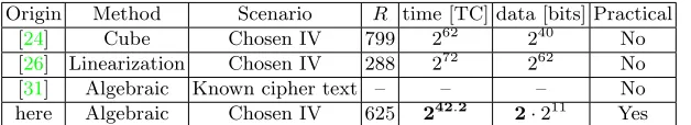
Origin Method Scenario R time [TC] data [bits] Practical
[24] Cube Chosen IV 799 262 240 No
[26] Linearization Chosen IV 288 272 262 No [31] Algebraic Known cipher text – – – No here Algebraic Chosen IV 625 242.2 2·211 Yes
Table 1: Relevant attacks on Trivium withRrounds, time- and data complexity. Time is measured in Trivium computations.
Basically, the most promising algorithms come from the F-family of Gr¨obner basis algorithms [20,19], see [3] for an overview. They have been successfully applied in the case of public key schemes [22,23], but also stream ciphers [21]. The main disadvantage is the high memory consumption. Although there are some counter examples for special cases, the running time of Gr¨obner basis algorithms is inherently exponential in the number of variables. Even worse, the memory consumption increases withO(nr) fornthe number of variables andrthedegree of regularity. In particular the latter makes Gr¨obner bases unusable for our purpose as we haver≥2 andn≈220. Still, we want to note a special and useful property of Gr¨obner basis algorithms that can also be found in our solver: If the system is unsolvable, the running time becomes significantly lower. This has been used in the so-called “hybrid strategy” from [7] to speed up the overall computation overF2. We will also exploit this, cf. Sec.3.4.
Another line of algorithms comes from the so called “XL—eXtended Linearization” [13]. Here, the main operation is multiplying all known equations with all monomials up to a certain degree. While these new equations are trivially true, some of them are linearly independent and can hence be used in a so-called Macaulay matrix to reduce the overall problem to linear algebra over F2. In a Macaulay matrix, the rows represent polynomials while the columns represent monomials, cf. [3] for an overview of the idea. Although it has been shown that techniques from the XL-family are strictly less efficient than from the F-family [40,39,5,17], XL does have its merits as it is easier to adapt to different settings. Hence we have used a specialized version of XL in our solver to improve its efficiency, cf. Sec.3.
Last but not least, there is the ElimLin algorithm [12,16] where linear equations are used to eliminate variables. After that, the system is simplified with linear algebra techniques, cf. Sec.3.1. It can handle large sparse polynomial systems with 3056 variables and 4331 monomials in 2900 equations and it is so simple that it can easily be tweaked for specific purposes. While this is possible—to some extent—for the XL-family, it is much more difficult to envision for the F-family described above. We have hence used ElimLin as the core for our solver, cf. Sec. 3.1. However, we want to stress thatplain ElimLin without further modifications is not efficient enough to deal with systems that arise from the modelling of Trivium.
1.3 Our contributions
Our first contribution are techniques to model many instances of Trivium as a quadratic equation system. We also introduce strategies to handle the large number of variables within this model. The modelling techniques and strategies can be applied to any symmetric cipher since the upcoming system of equation is structured according to the update function of the cipher.
The second contribution of this paper is a solver which is able to solve structured, sparse, quadratic equation systems. Based on ElimLin and eXtended Linearization we introduce a monomial order to have more control in the ElimLin-Step and change XL so that it preserves the monomial structure of the system. Furthermore we introduce a method that is able to make computations with higher algebraic degree while the result of this computations is still quadratic.
With the above mentioned techniques we settle an attack on a round reduced variant of Trivium with
2
Trivium
The main point of our attack is to get a suited algebraic system of equations overF2for a considered cipher. As soon as the modelling part is done, we will solve the system of equations with a special purpose solver, cf. Sec.3. We present our modelling techniques with the stream cipher Trivium from [10] as a testbed.
Trivium generates up to 264 keystream bits from an 80 bit IV and an 80 bit key. The cipher consists of an initialization or “clocking” phase ofRrounds and a keystream generation phase. ForR= 1152 we obtain thefull version as stated in [10], otherwise around-reducedvariant of Trivium, denoted by Trivium-R. There are several ways to describe Trivium—below we use the most compact one with three quadratic, recursive equations for the state bits and one linear equation to generate the output in the keystream generation phase.
2.1 Definition and direct considerations
Consider three shift registers A := (ai, . . . , ai−92), B := (bi, . . . , bi−83) and C := (ci, . . . , ci−110) of length 93,84 and 111 respectively. They are called thestate of Trivium.
First the state of Trivium is initialized with
A= (k0, . . . , k79,0, . . . ,0)
B= (v0, . . . , v79,0, . . . ,0) and
C= (0, . . . ,0,1,1,1).
Here (k0, . . . , k79) is the secretkey and (v0, . . . , v79) is the publicinitialization vector (IV)of Trivium. Before output is generated Trivium is updated R rounds according to the following three state update functions:
bi:=ai−65+ai−92+ai−90ai−91+bi−77,
ci:=bi−68+bi−83+bi−81bi−82+ci−86,
ai:=ci−65+ci−110+ci−108ci−109+ai−68.
ForR= 1152 we obtain the original variant from [10]. Since this variant have not been broken, round-reduced variants are used to evaluate the security margin of Trivium.
After this initialization phase Trivium generates one output bitzi per round by the function
zi:=ci−65+ci−110+ai−65+ai−92+bi−68+bi−83.
We producenobits of outputzi fori= (R+ 1). . .(R+no).
Recovering the initial vectorAis the prime aim of a key recovery attack. Note that the vectorsB, C are actually known to an attacker at the beginning of the initialization phase since the IV is public. Therefore we make the additional assumption that an attacker has control over the IV used within the cipher and obtain a stream of output bits for a fixed key and any choice of IV. This is calledchosen IV scenarioand is in line, e.g.with cube attacks.
To launch our attack, we use several output streams (Trivium instances) that share the same key but different values for the IV. We see in Sec.4that this will lead to successful attacks at Trivium-R.
Obviously, we need approx. 3RT +noT intermediate variables, respectively, if we want to representT instances of Trivium-R with no output bits each. Before discussing strategies for solving such rather large systems, we start with an observation on Trivium.
2.2 Similar variables
Let I ⊂ V be a subset of all IV variables V. We call I the master cube of the attack. In addition, we consider the first no output bits of Trivium initialized with the same key and all 0/1-combinations for variables in the master cubeI. All other IV variables are set to zero.
We set up all Trivium instances with symbolic key variables k0, . . . , k79. Denote the current Trivium instance by t ∈ N. We initialize these instances for a given number of roundsR and introduce three new variables for very roundifor the entriesat,i, bt,i andct,i in the three registersAt, BtandCt. This produces a quadratic system with a large number of variables and monomials.
Now we take a more general point of view and introduce similar variables for generalized systems of equations. In particular, we denote all intermediate variables byy0, y1, . . .
Definition 1. Let P = F2[k0, . . . , k79, y0, y1, . . .] =: F2[K, Y] be the Boolean polynomial ring in the key variablesK and all intermediate variablesY.
We call the two intermediate variablesyiandyjsimilar iffyi+yj =p(K, Y\{yi, yj}), wherep(K, Y\{yi, yj}) is a polynomial of degreedeg (p)≤1.
Following the definition, we check for similar variables whenever we should introduce a new intermediate variable. If the new variable is similar to one or a linear combination of many existing variables we continue computations without a new variable. Instead of using a new intermediate variable for quadratic monomials already introduced, we use a linear combination of existing variables.
In generic systems, similar variables could be not of much use. However, if all equations stem from one algebraic model for one given cipher, we are likely to find many similarities. The following example illustrates how we work with similar variables in the case of Trivium.
Example 1. Consider the polynomials
f0=y0+k78k79+k53
f1=y1+k77k78+k79+k52
inP.
These polynomials define intermediate variables y0, y1and form the system of equationF. Assume we want to introduce the intermediate variable y2 with
f2=y2+k79k78+k78k77+k5+k61.
It holds thaty2=y1+y0+k53+k79+k52+k5+k61. Therefore, we do not need to introducey2and can continue computation with y0 andy1. This does not only save us one variable, but we also have replaced a
quadratic equation by a (potentially more useful) linear one. ut
The nice aspect is that these variables carry through: As soon as we have concluded that all variablesbi,12 fori= 0..T−1 will always have the same value, we can replaceall of them in all polynomials by only one, say b0,12. Obviously, the same is true for bi,13 but also many other ones. When we have replacedbi,12bi,13 byb0,12b0,13, we obtain even more similar variables. Consequently, we obtain a substantially smaller number of monomials than before. Note that there are different ways of considering similar variables. In any case, we need a solver that can first identify them and second make use of them by replacing all linear relations within a given system.
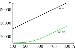
While the above definition captures any behavior for any system of equations, we see that it applies very well to Trivium, see Figure1 for some experimental results on Trivium-R. Here, we have generatedT = 32 instances of Trivium with no = 66 output bits. On thex−axis we see the number of initialization rounds; on the y−axis we have the total number of variables in use. As we can see the number of intermediate variables has greatly decreased; even for only 32 instances of Trivium. ForR= 600 rounds we also produce 66·32 = 2112 output equations. The model in [31] can just handle one instance of Trivium. So it would need 288 + 3·2112 = 6624 variables to produce that amount of output equations. When using more instances of Trivium we get even more efficient.
R ν
400 500 600 700 800 10000
30000 50000
with w/o
Fig. 1: Number of variables forT = 32 instances of Trivium andno= 66 output bits; Number of Rounds R against number of variablesν with and without similar variables
backwards and just generate the variables we need. This way, we just generate the variables and monomials that are needed. Note that this is contrary to earlier algebraic modellings of Trivium such as [32,31].
To evaluate our representation of Trivium, we made several experiments with the fast Gr¨obner basis PolyBoRi [9]. PolyBoRi is specialized on Gr¨obner basis for Boolean polynomial rings and uses a variant of Faug`ere’s F4 algorithm (see [20]).
We use a server node with a [email protected] processor and abort a computation if it exceeds 16 Gb of RAM or 24 hours of time. We tried to solve resulting systems of equations that represents
Trivium-R for varying number of rounds R with and without similar variables. Table 2 shows the results of the experiments.
R Similar variables Memory [Gb] Time [h] Note
150 No 8 <1
300 Yes 3 1 degrevlex
420 Yes 11 13 suited monomial ordering
Table 2: Experimental results for solving systems of equations based on Trivium-R for varying numbers of roundsR with and without similar variables. The suited monomial ordering is thedegrevlex-ordering with
k0< . . . < k79< a0,0< b0,0< c0,0< a1,0< b1,0< c1,0< . . . < cT−1,R−1 withT instances of Trivium.
Without similar variables we can solve a system of equations that represents Trivium-150, but we are not able to solve a system for R >160. Moreover, the behavior of PolyBoRi heavily depends on the chosen monomial ordering (like any Gr¨obner basis solver). The best we could do was Trivium-420 with a degrevlex-ordering andk0< . . . < k79 < a0,0< b0,0 < c0,0 < a1,0< b1,0< c1,0< . . . < cT−1,R−1 withT instances of Trivium. The system of equations has 1300 variables and 3900 monomials in 1500 equations. If we chose a different sorting of the variables we never got comparable results as indicated in Table2by solving Trivium-300 with adegrevlex-ordering. This was the only variant of Trivium that was solved consistently.
Thus solving polynomial systems arising for largeR is still out of reach for current Gr¨obner basis imple-mentations like PolyBoRi. The memory consumption is simply too high.
We have hence designed a solver which can handle such large numbers of equations and variables and will describe it in the following section.
3
Solving the system
Before going into details for the experiments, we describe our strategy to solve rather sparse systems over
aworking implementation than can handle around 106variables and 106equations, respectively, overF2. To the best of our knowledge, software with such special properties is not available at the moment. Our solver is organized around a specialized C++-core that natively handles quadratic polynomials over F2 and the
ElimLinandSLalgorithm. In addition, we have used several other building blocks which we describe in the remainder of the section. We report experimental results in Sec.4.
3.1 Main core
ElimLin orElimination of Linear variableshas been investigated in [12,16]. We generalize it with a monomial ordering, so the algorithm becomes
1. First we generate the Macaulay matrix for the system according to some monomial ordering τ.
2. Echelonize the matrix according to τ. This naturally splits up the system into linear equations L and quadratic equationsQ.
3. For each element p ∈ L, use the leading term LT(p). If there is at least one equation in Q that also contains the variable LT(p), eliminate LT(p) inQ.
4. If we substitute at least one variable inQ, go back to step 2.
We want to stress that ElimLin preserves the overall degree of our system Q. In addition, it automatically detects all similar variables (see def.1). Moreover ElimLin is able to deal with rather large but sparse systems of equations.
The original ElimLin algorithm did not have any ordering but used heuristics to determine which variable to eliminate in the non-linear part of the overall system. We found this approach fine for small systems but difficult to use for larger ones: The likelihood to fall into local optima was simply too high—even with advanced heuristics. Determining the correct order proved to be challenging and required careful experiments as can be seen in section2.2. Hence, we used thedegree reverse lexical (degrevlex) ordering. Note that this also works well in case of Gr¨obner basis algorithms. In the case of Trivium, we take the key variables first and sort the intermediate variables ascending according to rounds and instances of Trivium. We want to stress that the ordering is crucial in our analysis. Like in Gr¨obner techniques the results differ significantly depending on the ordering.
Sparse Linearization. ElimLin cannot conclude that a·b+a = 1 ⇒ a = 1, b = 0 for some variables
a, b∈F2 and therefore cannot solve arbitrary systems of equations. Hence we use a new variant of Extended Linearization that we callSparse Linearization.
In the XL-algorithm we multiply all quadratic polynomials with any monomial up to a degree D−2 that can be generated by the used variables. While these new equations are algebraically dependent, they can produce linearly independent rows in the Macaulay matrix. There is a variant for sparse systems called XSL in which systems of equations get multiplied by already used monomials. It has been used in the past to attack different cryptographic systems in [15].
Even XSL produces new monomials and increases the overall total degree of polynomial systems. Hence we may not use it for huge, structured systems of equations. The Sparse Linearization (SL)preserves the total degree and structure of the system by doing as follows:
We multiply each polynomial f in the polynomial systemF with any variableν contained in quadratic monomials off. If the total degree ofνf increases, we do not insert the new polynomial intoF. Further we check if all monomials ofνf are already used inF. If so, we insertνf into the system.
After SL is done we need to check for linear dependence of the new polynomials. We do this by the echelonization step of ElimLin.
F2directly but also implemented matrix-like operations (e.g.row addition) directly for polynomials. To this aim, each polynomial is stored as a (sorted) list of monomials rather than sparse vectors overF2. To make computations fast, we also keep a dictionary of lead terms, monomials in use by each polynomial and also a list of variables in use per polynomial. This way, addition of two polynomials with the same lead term and elimination of variables does not depend on the overall number of polynomials anymore. For speed, this part of the code is written in C++ (approx. 2500 lines).
M4RI. While the sparse strategy from above turned out to be efficient for sparse matrices, it fails if the ma-trices become increasingly dense. Note that this is inevitable when solving such a system: In all experiments, we had a degeneration from sparse to dense shortly before solving the overall system. To remedy this, we incorporated the fastest known, open source linear algebra package for matrices overF2, namely the Method of the 4 Russians Implementation (M4RI) [2]. Experimentally, we have found that matrices with less than≈ 1/1000 non-zero coefficients in the corresponding matrix over F2 should be handled by oursparse strategy described above and by M4RI otherwise.
3.2 Further building blocks
While the core is already pretty efficient, it can be made more suitable for solving systems of equations coming from Trivium-instances when coupled with the techniques below. Note that all these techniques have been implemented in Sage [36]. The full code (including test cases and comments) consists of≈6500 lines.
Sparse Target Linearization or STLis a generalization of the SL technique from above. Instead of limiting ourselves to degree-2 polynomials, we work with polynomials up to some degreed >2. In our calculations we are using a degree up tod= 4, which has proven optimal for equations coming from Trivium.
Analogous to SL, we multiply every polynomial f in F with any monomial µ in f. Afterwards we consider linear combinations of polynomials. Our target is to get new quadratic polynomials into the system while strictly bounding the number of new monomials in F in order to select good candidates we use the evolutionary strategy described below.
Note that we are working locally with a degree of regularity of 4. Here, locally means that we do not computeallsyzygies of degree three and four and we do not continue calculating with the polynomials with degree greater to 2. That is the main difference of STL and Gr¨obner basis algorithms (with a limited degree of regularity).
For random systems of equations, the STL strategy is doomed to fail due to the lack of useful quadratic equations afterwards. Our experiments show that it works fine for structured systems like Trivium, cf. Sec.4.
Evolutionary Strategy. To get the polynomials that should be used in the STL step we use a evolutionary strategy. We want to obtain (quadratic) equations that contains both key variables (xi) and output bits (zj). More generally: these equations should cover as many rounds of Trivium as possible. That means if we have an equation involving variablesarx and ary whererx< r and ry > Rwith r < Randas is a intermediate
variable introduced in roundswe want to maximizery−rx.
Unfortunately, it proved difficult to implement this strategy directly into the STL algorithm.
Guessing. In most cryptographic attacks, we start with some (deterministic) strategy to single out the promising keys and then bridge the gap for the full attack with brute force. We use the same strategy here by guessing the value of some variables and feed them into the overall solver before starting key recovery. To maximize the effect of the guessing step, we use the variables that occur most often in all polynomials system-wide. As expected, other selection strategies did not work that well for Trivium. More details on this idea are given in Sec.3.4.
3.3 Big picture
Online- and Offline-Phase. Our solving algorithm is divided into an online and an offline-phase (precom-putation). The main goal is to use trade-offs between the different algorithms. For example, the STL-step is quite powerful, but also quite slow. Hence, we only use it once and for all for a given, general system of equations (offline-phase). Once this system has been simplified, we insert all known output-bits, guessed variables and then recover the key. In detail we have
Offline: Generating the raw equations, ElimLin, SL, ES, STL and determine the variables which will be guessed later.
Online: Add guessed variables, output-bits, ElimLin and SL.
As mentioned above, the solver contains approx. 2500 lines of C++-code and approx. 6500 lines of Sage-code. Sage is a CAS described in [36]. It was used on an [email protected] with 256 nodes and 1 TB of RAM. Each node had access to at most 256 GB of RAM at a time. After the system has been simplified, the online-phase runs on a normal PC with 16 GB RAM.
Running the solver The above described parts of the solver varying significantly in running time. Therefore, our strategy to solve a polynomial system is to perform operations often if they can be executed quick.
In the offline phase we do the following.
LetF be the polynomial system that we want to solve. Our main tools are ElimLin and SL because they are most efficient. We perform one iteration of both algorithms and get the system F. We call F andF equal if they have the same echelonized Macaulay matrix. If F and F are not the same, we do another iteration until no change occurs or the system is solved. If no change occurs and the system is not solved, we do one iteration of STL and the evolutionary strategy. Afterwards we start with ElimLin and SL again.
Unlike Gr¨obner basis computation, our approach is heuristic. There is no guarantee that we will solve a polynomial system. We abort the computation if one of the following happens:
1. The polynomial systemF is solved.
2. No change occurred after an STL/evolutionary strategy step followed by ElimLin and SL. 3. The polynomial system is inconsistent.
In the online phase we do the same without the resource intensive steps STL and evolutionary strategy. Note that running the proposed solver is not equal to computing a Gr¨obner basis at degree 4. First, SL does not introduce new monomials to keep up sparsity of the polynomial system as long as possible. Even in Gr¨obner basis based algorithms forsparsesystems of equations we get new quadratic monomials of total degree two. That leads to a dense Macaulay matrix and therefore to increased memory usage. As described above, STL only uses a degree of regularity of fourlocally.
3.4 Scaling the attack
as the only factor for its simplicity. In particular, it is difficult to assign a sensible number for “memory” to a hardware implementation. Moreover, “memory” does not really speed up our attack but is a pure necessity: If we do not have enough memory, the attack does not work at all. Up to now, there are no clever ways to trade time for memory (or vice versa) using the solver described here.
All in all, we use a throughput oriented hardware implementation of Trivium (Table 2, Trivium64 in [25]) as basis for our comparison [25]. To the best of our knowledge, this is the fastest, throughput oriented implementation of Trivium. The authors report a throughput of B = 22.2996×10⁹ bps. To implement Trivium-R, we assume that we need to clock this implementation a total of (R+ 2) times on average: the firstR clocks for the preclocking phase and the other 2 clocks to derive 2 output bits on average. The last number is justified as follows: When the attacker learns the first output bit, she can terminate the brute force attack for around 1/2 of all keys. This goes on for all further bits. With the second output bit she can terminate the second half of all keys, with the third another half and so on. So we need on average two output bits to make our decision for someν= 80. . .100. So we have RB+2 Trivium applications per second. To scale up our attack, we assume that we guess a total ofrbits and achieve an overall time complexity (in Trivium computations) of
Tp:=
B((2r−1)T f+Ts)
R+ 2 ,
whereTsis the time of a successful computation of a solution andTf is the time our solver needs to recognize a failure in the guessed variables; both are average times for a given system. As we see,Tfis dominant in our computations. This is in line with other algorithms in this area such as [7]. Note that we assume that we get the data for all Trivium output as an input. So we do not calculate it which is a quite realistic assumption. Furthermore we know that we have a unique solution, namely the key of the cipher.
4
Experiments
This section consists of three parts. First we consider the model and we see a saturation of variables and mono-mials when adding Trivium instances. Second we present on some parameter studies to further strengthen our system of equations. Finally, we use our insights to actually attack Trivium using the techniques de-scribed in the previous sections. We stress that the overall system of equations can be generated before we get the actual data for the output. This way our attack splits into an online and offline phase as outlined in Sec. 3.4. All experiments were done on the cluster described in 3.3.As we do not use any parallelizing techniques we are only using one core. Furthermore we want to stress that the online phase only requires a standard computer with 16Gb of RAM.
Saturation. When adding different Trivium instances with identical key variables but different IV constants that lie in the same master cube, the overall number of variables and monomials in the quadratic monomials of the overall system tends towards a saturation point (cf. Fig. 2a–2b). More specifically; we fix 80−iIV bits to zero and set the remainingibits to all possible values fromFi2.
We have plotted saturation for 32 instances in Figures2a–2b, counting both the number of variables and the number of quadratic monomials needed for the system consisting of all instances of Trivium. In these figures, we have first added the IV with Hamming weight 0, then all IV with Hamming weight 1 and so forth. Note that instances with the same Hamming weight yield the same number of variables. As we can see in these graphs, the amount of variables needed to generate an instance becomes significantlylower if we generate instances with higher Hamming weight.
HW ν
01 2 3 4
1k 2k 3k 4k 5k
R= 500 R= 520 R= 540 R= 560 R= 580
(a) Hamming Weight against number of variablesν forR rounds of Trivium in a master cube of dimen-sion 5
HW µ
01 2 3 4
10k 20k 30k 40k 50k 60k
R= 510 R= 530 R= 550 R= 570 R= 590
(b) Hamming Weight against number of quadratic monomials µ forR rounds for Trivium in a master cube of dimension 5
Fig. 2: Saturation in the model of Trivium
Hamming weight. While this seems obvious when looking at the generating equations, it is still interesting to see howstrongthis effect is in practice. Unfortunately, we were unable to derive a closed formula depending on the number of instances and rounds but have to leave this as an open question.
In conclusion, saturation means that we can obtain more defining equations from many instances than we would expect from one instance alone. In a sense, this is the key observation to launch our attack.
Saturation should occur in other ciphers as well since the system of equation is generated by a repeatedly execution of an update function.
Note that we did not take the output equations into account yet but only those equations defining the system itself. While the output introduces additional, unknown monomials it will not add new variables as we will see in the next paragraph.
Output and parameters. While output equations clearly help us to linearize the system, the very structure of Trivium in our model yields a lot of additional monomials. Therefore, we do not add additional values for output equations or the output equations at all until the full (structural) system is completely simplified. Consider the output function:
zi:=ci−65+ci−110+ai−65+ai−92+bi−68+bi−83.
It uses 6 state bits from different rounds. If we insert for either of these state bits it produces 5 more monomials for each occurrence of the corresponding state bit in a quadratic monomial. Hence using more output bits per instance leads to far more monomials than we can afford.
Figure 3 compares systems with T = 64 instances and increasing number of rounds R. In the first experiment we used no = 1 and in the second no = 66. We see that many output bits do not necessarily lead to a more useful system because we get much more monomials. Even if we use two output equations we get a system with nearly double the number of monomials which we cannot solve easier. Note that figure 3
reflects the monomials needed for one instance while figure 2bshows the number of monomials needed for the whole system of equations. Therefore the saturation can also be seen in figure3.
When we useno= 66 output bits the number of monomials atR= 700 rounds is negligibly smaller than the number of monomials for full Trivium (R= 1152). We chooseno = 66 because forno>66 we need to introduce new intermediate variables even for the output and that destroys the purpose of (over)defining the system for the linearization step. Forno = 1 output bits, the same effect occurs forR= 925 rounds. Since we want to linearize our system to derive a solution we get the following conjecture.
R µ
525 700 900 1150
10000 20000 30000 40000 50000 60000
000100
011000
111111
(a) Initialization rounds R against number of quadratic monomialsµforno= 1
R µ
525 700 900 1150
10000 20000 30000 40000 50000 60000
000100
011000
111111
(b) Initialization rounds against number of quadratic monomialsµforno= 66
Fig. 3: Comparing monomials withno= 1 andno= 66; Initialization roundsRagainst number of quadratic monomialsµ; The numbers next to the lines are the significant parts of the IV (binary). The rest of the IV is zero. Consider the Hamming weight of these numbers.
In a nutshell: Since the number of monomials does not increase, neither does the difficulty of the attack. Unfortunately, both settings are out of reach for a practical test at the moment.
In addition, we obtained the following result: When choosing 2i instances of Trivium, it is optimal to arrange them in a master cube rather than sampling them “at random” from all possible 280IV. In particular, such a system becomes fully unsolvable with our methods.
Attacks. In this paragraph we describe the attacks and their complexities.
In Figure3we have illustrated the number of monomials depending on the number of output bits. With this in mind we have specialized our attack to the case no = 1. Based on this, we generate a system with Trivium-625 instances.
The following table shows the number of monomials and variables needed for the full system. This also includes “dummy” variables for the output. When we add concrete data for the output bits to our system these numbers decrease rapidly. Furthermore we can see that there is a time-data trade-off when guessing variables. When we guess fewer variables we need more data to launch the attack. When we guess more variables we need less data but the time complexity increases.
R µ ν #guessed variables data complexity time complexity 625 499,741 15,869 23 211 259.7 625 1,135,858 32,518 0 2·211 242.2
Table 3: Experimental results from the Online-phase on Trivium-625 with number of variablesνand number of monomialsµ. Time is measured in Trivium computations.
When our guess was incorrectly, it takes our solver on average 211.6 seconds to report that the system was inconsistent. However, when we guess correctly the system is solved in 213.8 seconds on average.
than brute force (280). We note that we do not actually compute the guessing step of this attack since it is not feasible to do so.
When we do not guess variables, we need more data and though more instances in our symbolic system. Generating the full symbolic system becomes a challenge due to the size of the system and RAM usage in the offline-phase. Thus we generate two systems consisting of 211instances each. The two systems do not profit from each other through similar variables in the offline-phase so the number of variables and the number of monomials is more than doubled. In the online-phase of the attack each system is reduced due to the linear output equations and similar variables. In our example in the table above we solved the system in 217.1 seconds which leads to 242.2 Trivium computations on average. Again, this experiment was conducted 101 times.
Unfortunately, we are unable to find a closed formula to predict the number of instances we would need to solve a system for a given number of rounds, as the behaviour of Trivium and the solver is quite erratic in this respect.
The real bottleneck of our attack is the generation of a symbolic system for a useful number of instances in the offline-phase. We can overcome this problem with a better implementation of the linear algebra or the ElimLin algorithm. However, we still cannot really resolve the exponential growth starting at R= 700 (Fig. 3) which works as a kind of barrier for our techniques used to attack Trivium. We want to encourage others to further improve or enhance the techniques used in this paper.
5
Conclusions
In this paper we have shown that algebraic attacks can be significantly improved. We achieve this by enhanc-ing the ElimLin algorithm with a variant of eXtended Linearization and usenhanc-ing a proper monomial orderenhanc-ing; in particular the last proved crucial in our experiments. Overall, we built a solver for sparse polynomial sys-tems that can handle up to 106monomials in 106equations. In particular, we solved the system of equations arising from Trivium-625 with 1,135,858 monomials and 32,518 variables. Before our work, plain ElimLin was able to solve systems of equations with 3056 variables and 4331 monomials. While this is not quite com-parable, because the systems solved are not the same, this improvement by a factor of≈262 demonstrates considerable progress.
In addition, we have seen that using many instances of Trivium rather than only one with a long key stream significantly improves the attack. All in all, we were able to break a 625 round reduced version of Trivium in practical time (242.2 Trivium computations) and a data complexity of 212. Other key recovery attacks on Trivium can do better in terms of rounds withR= 799 but they requires a large amount of data (240 bits) and time 262 while guessing 62 bits. It is doubtful if this rate can be achieved in practice. An advantage of our approach is that we actually computed the full attack and did not make extrapolations from our results, as we do not want to make promises which are hard to keep.
An open questions is the existence of weak keys. They would improve our attack by reducing the overall number of monomials. While some experiments point at their existence they still elude a full characterization. Another line of research is the integration of more toolboxes into our solver, most notably SAT-solvers and more efficient sparse linear algebra packages.
While our experiments were conducted only on Trivium, we are confident that the ideas and lessons learned are also useful for the algebraic cryptanalysis of other symmetric primitives, such as block ciphers or hash functions. We want to stress that the potential of algebraic cryptanalysis can only be unleashed if equal stress is put on modelling techniques and the corresponding solver.
References
1. ECRYPT II Yearly Report on Algorithms and Keysizes (2011-2012), rev. 1.0. http://www.ecrypt.eu.org/ documents/D.SPA.20.pdf(Date: 2012-09-30 2012)
2. Abbott, T., Albrecht, M., Bard, G., Bodrato, M., Brickenstein, M., Dreyer, A., Dumas, J.G., Hart, W., Harvey, D., James, J., Kirkby, D., Pernet, C., Said, W., Wood, C.: M4RI(e)—Linear Algebra overF2 (andF2e). http:
//m4ri.sagemath.org/
3. Albrecht, M.: Algorithmic Algebraic Techniques and their Application to Block Cipher Cryptanalysis. Ph.D. thesis, Royal Holloway, University of London (2010)
4. Armknecht, F., Krause, M.: Algebraic Attacks on Combiners with Memory. In: CRYPTO. Lecture Notes in Computer Science, vol. 2729, pp. 162–175. Springer (2003)
5. Ars, G., Faug`ere, J.C., Imai, H., Kawazoe, M., Sugita, M.: Comparison between XL and Gr¨obner basis algorithms. In: ASIACRYPT 2004, LECTURE. pp. 338–353. Springer-Verlag (2004)
6. Aumasson, J.P., Dinur, I., Meier, W., Shamir, A.: Cube Testers and Key Recovery Attacks on Reduced-Round MD6 and Trivium. In: FSE 2009, Fast Software Encryption. pp. 1–22. Springer (2009)
7. Bettale, L., Faug`ere, J.C., Perret, L.: Hybrid approach for solving multivariate systems over finite fields. In Journal of Mathematical Cryptology 3, 177–197 (2009)
8. Biryukov, A., Canni`ere, C.D.: Block ciphers and systems of quadratic equations. In: FSE. Lecture Notes in Computer Science, vol. 2887, pp. 274–289. Thomas Johansson, editor, Springer (2003), iSBN 3-540-20449-0 9. Brickenstein, M., Dreyer, A.: PolyBoRi: A framework for Groebner-basis computations with Boolean polynomials.
Journal of Symbolic Computation 44(9), 1326 – 1345 (2009),http://dx.doi.org/10.1016/j.jsc.2008.02.017, effective Methods in Algebraic Geometry
10. Cannire, C.D., Prenel, B.: Trivium. In: New Stream Cipher Designs, LNCS, vol. 4986, pp. 84–97. Springer (2008) 11. Cid, C., Murphy, S., Robshaw, M.J.B.: Small Scale Variants of the AES. In: FSE. Lecture Notes in Computer Science, vol. 3557, pp. 145–162. Henri Gilbert and Helena Handschuh, editors, Springer (2005), iSBN 3-540-26541-4
12. Courtois, N.T., Bard, G.V.: Algebraic Cryptanalysis of the Data Encryption Standard. In: Cryptography and Coding, Lecture Notes in Computer Science, vol. 4887, pp. 152–169. Springer Berlin Heidelberg (2007)
13. Courtois, N.T., Klimov, A., Patarin, J., Shamir, A.: Efficient Algorithms for Solving Overdefined Systems of Multivariate Polynomial Equations. In: Advances in Cryptology — EUROCRYPT 2000. Lecture Notes in Computer Science, vol. 1807, pp. 392–407. Bart Preneel, editor, Springer (2000), extended Version: http: //www.minrank.org/xlfull.pdf
14. Courtois, N.T., Meier, W.: Algebraic Attacks on Stream Ciphers with Linear Feedback. In: Proceedings of the 22Nd International Conference on Theory and Applications of Cryptographic Techniques. pp. 345–359. EURO-CRYPT’03, Springer-Verlag (2003)
15. Courtois, N.T., Pieprzyk, J.: Cryptanalysis of Block Ciphers with Overdefined Systems of equations. In: ASIA-CRYPT. pp. 267–287 (2002)
16. Courtois, N.T., Sepehrdad, P., Susil, P., Vaudenay, S.: Elimlin Algorithm Revisited. In: Fast Software Encryption—FSE 2012. pp. 306–325 (2012)
17. Diem, C.: The XL-Algorithm and a Conjecture from Commutative Algebra. In: ASIACRYPT. Lecture Notes in Computer Science, vol. 3329, pp. 323–337. Springer (2004)
18. Dinur, I., Shamir, A.: Cube Attacks on tweakable black box polynomials. In: EUROCRYPT. Lecture Notes in Computer Science. vol. 5479, pp. 278–299. Springer (2009)
19. Faug`ere, J.C.: A new efficient algorithm for computing Gr¨obner bases without reduction to zero (F5). In: In-ternational Symposium on Symbolic and Algebraic Computation — ISSAC 2002. pp. 75–83. ACM Press (Jul 2002)
20. Faug`ere, J.C.: A New Efficient Algorithm for Computing Grbner Bases (F4). In: IN: ISSAC 02: PROCEEDINGS OF THE 2002 INTERNATIONAL SYMPOSIUM ON SYMBOLIC AND ALGEBRAIC COMPUTATION. pp. 75–83. Springer (2002)
21. Faug`ere, J.C., Ars, G.: An Algebraic Cryptanalysis of Nonlinear Filter Generators using Gr¨obner bases. Rapport de recherche 4739 (Feb 2003),www.inria.fr/rrrt/rr-4739.html
22. Faug`ere, J.C., Joux, A.: Algebraic Cryptanalysis of Hidden Field Equation (HFE) Cryptosystems Using Gr¨obner Bases. In: In Advances in Cryptology CRYPTO 2003. pp. 44–60. Springer (2003)
24. Fouque, P., Vannet, T.: Improving Key Recovery to 784 and 799 rounds of Trivium using Optimized Cube Attacks. FSE 2013, Fast Software Encryption (2013)
25. Good, T., Benaissa, M.: Hardware performance of eStream phase-III stream cipher candidates. SASC 2008 - The State of the Art of Stream Ciphers (2008),http://www.ecrypt.eu.org/stvl/sasc2008/, pages 163–173 26. Khazaei, S., Hasanzadeh, M.M., Kiaei, M.S.: Linear Sequential Circuit Approximation of Grain and Trivium
Stream Ciphers. Cryptology ePrint Archive, Report 2006/141 (2006),http://eprint.iacr.org/2006/141/
27. Knellwolf, S., Meier, W., Naya-Plasencia, M.: Conditional Differential Cryptanalysis of Trivium and KATAN. In: Selected Areas in Cryptography. pp. 200–212 (2011)
28. Lim, C.W., Khoo, K.: An Analysis of XSL Applied to BES. In: Fast Software Encryption, FSE 2007. Lecture Notes in Computer Science, vol. 4593, pp. 242–253. Springer (2007)
29. Murphy, S., Robshaw, M.J.: Essential algebraic structure within the AES. In: Advances in Cryptology — CRYPTO 2002. Lecture Notes in Computer Science, vol. 2442, pp. 1–16. Moti Yung, editor, Springer (2002) 30. Quedenfeld, F., Wolf, C.: Algebraic Properties of the Cube Attack. Cryptology ePrint Archive, Report 2014/800
(2014),http://eprint.iacr.org/2014/800/
31. Raddum, H.: Cryptanalytic results on Trivium (2006), http://www.ecrypt.eu.org/stream/triviump3.html 32. Schilling, T., Raddum, H.: Analysis of Trivium using compressed right hand side equations. In: Information
Security and Cryptology. Lecture Notes in Computer Science. vol. 7259, pp. 18–32. Springer (2012)
33. Shannon, C.E.: Communication theory of secrecy systems. Bell System Technical Journal 28, 656–p715 (4th October 1949)
34. Simonetti, I., Faug`ere, J.C., Perret, L.: Algebraic Attack Against Trivium. In: First International Conference on Symbolic Computation and Cryptography, SCC 08. pp. 95–102. LMIB, Beijing, China (April 2008), http: //www-polsys.lip6.fr/~jcf/Papers/SCC08c.pdf
35. Stankovski, P.: Greedy Distinguishers and Nonrandomness Detectors. In: INDOCRYPT. pp. 210–226 (2010) 36. Stein, W., et al.: Sage Mathematics Software (Version 6.1). The Sage Development Team (2014),
http://www.sagemath.org
37. Sugita, M., Kawazoe, M., Perret, L., Imai, H.: Algebraic Cryptanalysis of 58-Round SHA-1. In: FSE. Lecture Notes in Computer Science, vol. 4593, pp. 349–365. Springer (2007)
38. Teo, S., et al.: Algebraic analysis of Trivium-like ciphers (2013), http://www.eprint.iacr.org/2013/240.pdf 39. Yang, B.Y., Chen, J.M.: All in the XL family: Theory and practice. In: ICISC 2004. pp. 67–86. Springer (2004) 40. Yang, B.Y., Chen, J.M.: Theoretical analysis of XL over small fields. In: ACISP 2004. LNCS, vol. 3108, pp.