Dataset Watermarking Using Hybrid Optimization and ELM

Dataset Watermarking Using Hybrid Optimization

and ELM

Vithyaa Raajamanickam

_{,Ms.R. Mahalakshmi}

Assistant Professor, Park's college Chinnakarai,Tirupur 641605

Abstract— The large datasets are being mined to extract hidden knowledge and patterns that assist decision makers in making effective, efficient, and timely decisions in an ever increasing competitive world. This type of “knowledge-driven” data mining activity is not possible without sharing the “datasets” between their owners and data mining experts (or corporations); as a consequence, protecting ownership (by embedding a watermark) on the datasets is becoming relevant. The most important challenge in watermarking (to be mined) datasets is: how to preserve knowledge in features or attributes? Usually, an owner needs to manually define “Usability constraints” for each type of dataset to preserve the contained knowledge. The major contribution of this paper is a novel formal model that facilitates a data owner to define Usability constraints—to preserve the knowledge contained in the dataset—in an automated fashion. The model aims at preserving “classification potential” of each feature and other major characteristics of datasets that play an important role during the mining process of data; as a result, learning statistics and decision-making rules also remain intact.

The proposed paper is implemented with hybrid algorithm using Genetic Algorithm (GA) and Particle Swarm Optimization (PSO) for selecting global datasets, classification of tuples to be watermarked by Extreme Learning Machine (ELM). The proposed paper not only preserves the knowledge contained in a dataset but also significantly enhances watermark security compared with existing techniques."

1. INTRODUCTION

From large databases, datasets are generated. These datasets are used to extract information and this information is used in an effective manner for decision makers. These datasets are used by an effective organisation and also used by the business people to find the novel solution for their problems [1].

Watermarking is mostly used as one of the methods in data mining to embed additional information which is not in visible form. Watermarking for database is used in several areas. First well-known database watermarking scheme for relational database is implemented in [2].

This type of watermarking can be applied to any database relation and that having attributes. To preserve the knowledge of the database, ability of the feature is enhanced to preserve the attributes. Also the dataset classification accuracy remains intact.

The process of defining “Usability constraints” is dependent on the dataset and its intended applications.

Sharing the datasets in emerging field and protecting the owner’s dataset is an important and one of the challenging tasks in the database. Watermarking is one of the common mechanisms used in database to elevate and proof the ownership database such as e audio, video, image, relational database, text and software [3]–[5]. “Usability constraints” is a challenge because a user has to strike a balance between “robustness of watermark” and “preserving knowledge contained in the features”.

2. . RELATED WORK

In [6] author proposed a technique for watermarking numeric attributes in a database.

One of the watermarking embed technique was implemented in [7].This technique is used to embed the watermarking scheme into a dynamic data structure. This method proves better due to their effectiveness and this method is projected through Java software.

In [8] proposed a tuple based watermarking techniques for relational database. This type of technique is not used for data mining dataset because it does not preserve the data mining information.

3. FORMAL MODEL FOR “USABILITY CONSTRAINTS” To define “Usability Constraints” that preserves the knowledge during the process of inserting watermark in the dataset.

Definition 1. Tuple: A tuple is an ordered list of elements. The tuple is used as a basic unit for referring different parameters of a dataset.

Definition 2. Learning Algorithm: Given a dataset D

with M features, N instances, and a class attribute Y, a learning algorithm Ґ, groups instances into different groups. Formally

Ґ: D → (C , C )

In the above equation α is the number of distinct items in Y. A learning algorithm may be a classification algorithm or a clustering algorithm.

Definition 3. Learning Statistics: C Learning statistics is a tuple containing the classification statistics (or accuracy) of a particular learning algorithm. Formally:

C ← Ґ: D

TP = TP

TP + FN × 100

FP = × 100

Decision rule boundaries denote the threshold values that define the boundary of a particular decision rule.

TP (true positive): TP denotes the number of instances of a particular class detected as instances of that class.

FP (false positive): For a particular class, the number of instances of other class (es) detected as instances of that particular class.

TN (true negative): For a particular class, the number of instances detected as instances of other class(es).

FN (false negative): For a particular class, the number of instances of that class detected as instances of other class (es).

Then store the learning statistics in C , that is:

C = (TP , FP , R )

Definition 4. Decision Rules: Given a dataset D with M features, a rule is a tuple constructed by mapping of m features, with m ⊆ M, based on C for identifying the class label y, where y ∈ Y, R contains all such rules as:

R: (D , C ) → Y

Definition 5. Feature Selection Scheme: A feature selection scheme S transforms M-dimensional data D , having N samples, M features and a class attribute , in m-dimensional space R (with m ≤ M , such that R ⊆ R ) that can yield “optimum” learning statistics. Formally,

S: D → R

4. .PROPOSED FRAMEWORK

The proposed frame work is divided into several steps.

1. Pre-processing is used to remove the unwanted datas like missing values, incorrect and noisy datas.

2. Selection of global dataset from the given datasets is done using optimization method of PSO and GA.

3. Applying watermark to the features of selected global dataset.

4. The row values to be watermarked are classified using ELM.

5. Applying watermark to the row values that are greater than the given kernel point.

Selection of Dataset through Optimization Method

This optimization method is used to select the dataset for watermarking process. In this paper hybrid method is selected to process the framework. Using this hybrid method, best dataset is selected from the given four datasets.

The hybrid optimization for dataset watermarking is performed with PSO & GA. Genetic algorithm(GA) is one of the recognized powerful techniques for optimization and global search problems. It was originated in 1970 by John Holland. Here the process involved in the genetic evolution such as natural selection, mutation and crossover are developed for the target problems. For optimization problems,

GA populations are formulated as chromosomes of candidate solution. This technique maintains a population of M individuals Pop(g) = X (g), … , X (g) for each iteration g. The potential solution of the population is denoted by each individual. Using selection process, new populations are obtained and these are all based on individual adaptation and some genetic operators. In each generation, the fitness of every individual in the population is evaluated. Depending on mutation and crossover, new individuals are generated and reproduced. Further in the genetic operation process, new tentative populations are formed by selecting individuals and this selection process is repeated several times. Then from this process some of the new tentative population undergoes transformation. After the selection process, crossover creates two new individuals by combining parts from two randomly selected individuals of the population. The system needs high crossover probability and low mutation for good GA performances as an output. Mutation is a unitary transformation which creates with certain probability, p , a new individual by a small change in a single individual.

Below algorithm gives the methodology of the proposed hybrid algorithm. In selection process of the genetic algorithm, Particle Swarm Optimizaation (PSO) method is introduced. This algorithm is implemented in 1995 by

Kennedy and Eberhart and this is one of the well known optimization techniques. In PSO, each particle represents a candidate solution within a n-dimensional search space. The position of a particle i at iteration t is denoted by x (t) =

x , x , … , x .

For each iteration, every particle moves through the search space with a velocity v (t) = v , v , . . , v calculated as follows

v (t + 1) = wv (t) + c r y (t) − x (t) + c r y (t) − x (t)

In the above equation dimension of the search space is denoted by j and j ∈ 1,2, … , n, inertia weight is given by w,

y (t) is the personal best position of the particle i at iteration t and y(t) is the global best position of the swarm iteration t.

p is the personal best solution and it denotes the best position found by the particle search process until the iteration t. p is the global best position and it identifies the best position found by the entire swarm until the iteration t.

Acceleration coefficient and random numbers are given by parameters c , c , r and r . v , v is the limited range for the velocity. . After updating velocity, the new position of the particle i at iteration t+1 is calculated using the following equation:

x (t + 1) = x (t) + v (t + 1)

w(t) = w − t ×(w − w ) t

5. .CLASSIFICATION

The rows to be watermarked are classified using Extreme Learning Machine.

Learning algorithm uses a finite number of inputs and outputs for training in supervised batch learning system. In this system, consider N arbitrary distinct samples(X , t ) ∈ R × R , in this X is an n × 1 input vectors and t is an

m × 1 target vector. If an SLFN with N hidden nodes can approximate these N samples with zero error, it then implies that there exist β , a and b such that

f X = β G a , b , X = t , j = 1, … , N

The above equation can be written as

Hβ = T

Where

H(a , … , a , b , … , b , X , … , X )

=

G(a , b , X ) … G(a , b , X )

: … :

G(a , b , X ) … G(a , b , X ) _×

β = β

: β

×

and T = t: t _×

H is called the hidden layer output matrix of the network [14], the ith column of H is the ith hidden node’s output vector with respect to inputs X , X , … , X and the jth row of H is the output vector of the hidden layer with respect to input

X .

In real applications, the number of hidden nodes N, will always be less than the number of training samples N, and hence the training error cannot be made exactly zero but can approach a nonzero training error ∈. The hidden node parameters a and b(input weights and biases or centres and impact factors) need not be tuned during training and may simply be assigned with random values according to any continuous sampling distribution [11], [12], [13]. Equation (5) then becomes a linear system and the output weights β are estimated as

β = H T

Where H the Moore-Penrose is generalized inverse [15] of the hidden layer output matrix H. The ELM algorithm which consists of only three steps, can then be summarized as

ELM Algorithm: Given a training set

ℵ = (X , t )|X ∈ R , t ∈ R , i = 1, … , N , activation function g(x), and hidden node number N.

STEP 1: Assign random hidden nodes by randomly generating parameters (a , b ) according to any continuous sampling distribution, i = 1, . . , N.

STEP 2: Calculate the hidden layer output matrix H. STEP 3: Calculate the output weight β

β = H T

Recently in [9] have developed a new learning algorithm called Extreme Learning Machine (ELM) for Single-hidden Layer Feed forward neural Networks (SLFNs). In this

technique hidden node parameters are randomly chosen and fixed and then analytically determine the output weight of SLFNs [10].

Single-hidden Layer Feed forward neural Networks

N hidden nodes are the output of an SLFN and this can be represented by

f (X) = β G(a b X), where XϵR , a ϵR

In this equation, the learning parameters of hidden nodes are given by a and b , then β indicates the weight connecting the ith hidden node to the output node. Output of the ith hidden node with respect to the input x is given byG(a b X).

For additive hidden node with the activation function

g(x): R → R, G(a b X) is given by

G(a b X) = g(a . X + b ), where b ∈ R

In the above equation a is the weight vector connecting the input layer to the ith hidden node and b is the bias of the ith hidden node . X indicates the inner product of vectors a

and X in R . For an RBF hidden node with an activation function g(x): R → R, G(a b X) is given by

G(a b X) = g(b ‖X − a ‖, b ϵR )

In the above equation a and b are the center and impact factor of the ith RBF node. R indicates the set of all positive real values. The RBF network is a special case of SLFN with RBF nodes in its hidden layer. Each RBF node has its own centroid and impact factor and its output is given by a radially symmetric function of the distance between the input and the center.

6. WATERMARKING SCHEME

In this paper proposed a watermarking scheme that preserves the classification potential of features. There are two main phases in watermarking scheme: watermark encoding and watermark decoding.

The classification potential of each feature is calculated using mutual information and it is stored in a vector. The threshold is computed using a vector of classification potentials. The classification potential of features (the vector) are then used to logically group features of the dataset into non overlapping groups. The watermark is optimized and embedded in this stage while enforcing the usability constraints modelled.

Data grouping step is not performed for nonnumeric features because watermark embedding algorithm does not bring any change in the values of such features. To embed a watermark in the dataset, a sequence of binary bits are used as a watermark. For watermarking a nonnumeric feature f, secret hash value for each row is calculated by seeding a pseudo random sequence generator ∂ with concatenation of a secret key K , class label of the row, and row value (ascii) as:

row, hash = ∂(K ‖y‖row, val)

7. . EXPERIMENTAL RESULTS

In this paper, implementation on different datasets chosen from different domains are performed and the respective datasets for this paper are multiclass dataset, high dimensional dataset and some missing values. The experiments are implemented on Java Platform. In this paper Optimization technique of dataset watermarking was implemented using hybrid algorithm of GA with PSO and the results are classified using ELM.

Figure 1: Initial Process

Figure 2: Current Status of the Proposed Framework

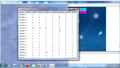
Figure 3:Dataset Preprocessing

Figure 4: Uploading Files

Figure 5: Information Message

Figure 6: Breast Cancer Dataset After Preprocessing

Figure 8: New thyroid after preprocessing

Figure 9: Sick Dataset After preprocessing

Figure 10: Dataset selection process

Figure 11: Data before preprocesing

Figure 12: Data after Preprocessing

Figure 13: Apply optimation algorithm

Figure 14: Grouping the process

Figure 16: Results

Figure 17: PSO Calculation

Figure 18: Selection dataset for constraints

Figure 19:Watermarking process

Figure 20:Message for Watermarking completion

Figure 1 to 20 gives the proposed framework results. Different dataset pre-processing results are illustrated in the above figures. After pre-processing, optimization techniques are used.

8. CONCLUSION

The proposed framework implemented a novel knowledge-preserving and lossless usability constraints model and a new watermarking scheme has been proposed for watermarking data mining datasets. In existing system, PSO algorithm is implemented, but it produces some drawbacks that the swarm may prematurely converge. The underlying principle behind this problem is that, for the global best PSO, particles converge to a single point, which is on the line between the global best and the personal best positions. To overcome the limitations of PSO, hybrid algorithms with GA are proposed. The basis behind this is that such a hybrid approach is expected to have merits of PSO with those of GA. One advantage of PSO over GA is its algorithmic simplicity. Another clear difference between PSO and GA is the ability to control convergence. The proposed framework optimizes the watermark embedding such that all usability constraints remain intact.

REFERENCES

[1] Kaggle’s contests: Crunching Numbers for Fame and Glory 2012[online]. [2] Rakesh Agrawal and Jerry Kiernan. Watermarking relational databases. In

28th Int Conference on Very Large Databases, Hong Kong, pages 155–166, 2002.

[3] R. Agrawal, P. Haas, and J. Kiernan, “Watermarking relational data: Framework, algorithms and analysis,” The VLDB Journal, vol. 12, no. 2, pp. 157–169, 2003.

[4] J. Palsberg, S. Krishnaswamy, M. Kwon, D. Ma, Q. Shao, and Y. Zhang, “Experience with software watermarking,” in Proc. 16th Ann. Computer Security Applications Conf., 2000, pp. 308–316.

[5] M. Atallah, V. Raskin, M. Crogan, C. Hempelmann, F. Kerschbaum, D. Mohamed, and S. Naik, “Natural language watermarking: Design, analysis, and a proof-of-concept implementation,” in Information Hiding. New York, NY, USA: Springer, 2001, pp. 185–200.

[6] R Agrawal and J Kiernan,” Watermarking relational databases”, in proc.28th Int. conf. Very Large Databases, 2002, pp. 155-166.

[7] R Sion, M Atallah and S Prabhakar, “Rights protection for relational data,” IEEE Trans. Knowl. Data Eng., vol.16, no.12, pp. 1509-1525, Dec. 2004. [8] J Palsberg, S Krishnaswamy, D Ma, M Kwon, Q Shao and Y

Zhang,”Experience with software watermarking”, in Proc. 16th computer security applications conf. 2000, pp. 308-316.

[9] G. Tang and A. Qin, ECG de-noising based on empirical mode decomposition, in: 9thInternational Conference for Young Computer Scientists, 2008, pp. 903–906.

[10] M. Alfaouri and K. Daqrouq, ECG signal denoising by wavelet transform thresholding, American Journal of Applied Sciences 5 (3) (2008) 276–281. [11] M. Blanco Velascoa, B. Weng, K. Barner, ECG signal denoising and

baseline wander correction based on the empirical mode decomposition, Comput. Biol. Med, pp.1–13, 2008.

[12] H. Liang, Z. Lin and F. Yin, Removal of ECG contamination from diaphragmatic EMG by non linear analysis, Non linear Anal, pp. 745–753, 2005.

[13] H. Liang, Q. Lin and J. Chen, Application of the empirical mode decomposition to the analysis of esophageal manometric data ingastro esophageal reflux disease, IEEE Trans. Biomed. Eng, pp.1692–1701. 2005. [14] P.E. Tikkanen, Non linear wavelet and wavelet packet denoising of

electro-cardiogram signal, Biol. Cybern, pp. 259–267, 1999.