Design and Development of Halbach Electromagnet
for Active Magnetic Bearing
Kootta P. Lijesh* and Harish Hirani
Abstract—Active Magnetic Bearings (AMBs) are advantageous due to their active control on rotor position, but are disadvantageous due to their high initial as well running costs. The running cost of AMB can be reduced by improving design of electromagnet so that the same magnetic field can be generated with reduced supply of electric current. In the present paper, analyses of various arrangements of electromagnets using 2D finite element (FE) have been presented. To validate the results of magnetic flux density obtained from theoretical study, experiments were performed, and comparisons have been presented. The electromagnet using Halbach winding arrangement provides the best results.
1. INTRODUCTION
The applications of Magnetic Bearings (MBs) are increasing due to their non-mechanical contact and low friction operation [1–5] support. The magnetic bearings are broadly classified as Passive Magnetic Bearings (PMBs) and Active Magnetic Bearings (AMBs). Due to brittleness [6], instability and low load carrying capacity [7] of PMBs, usage of AMBs [8, 9] is recommended. These bearings have built-in fault diagnostics [10, 11]. Shankar et al. [12] concluded that it is hard to justify the usage of AMBs, which costs minimum of $1500 compared to similar sized greased lubricated rolling element and hydrodynamic bearings which cost lesser than $15. Further Shankar et al. [12] compared the power loss among these bearings. As per their study for a typical application, AMBs consumed 48 W compared to 7 W consumed by rolling element bearing. However, such losses in running conditions of AMBs can be reduced by improving the design of electromagnet.
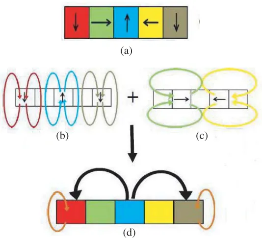
In PMBs, the flux density of a magnet can be increased without changing the volume of magnets using stacking arrangements [13–16], well known as Halbach arrangement. In this arrangement the magnetic flux density is added on one side and reduced on the opposite side. In PMBs, two types of Halbach arrangements have been tried (i) full Halbach array consists of five magnets [14] and (ii) half Halbach array consists of three magnets [15]. The increase in the magnetic flux of the Halbach magnetic arrangement is depicted in Figure 1.
In Figure 1(a), the direction of polarization of magnets is shown by the arrows. Figure 1(b) shows the magnetic field lines for radially polarized magnets, and Figure 1(c) shows the magnetic field lines for axially polarized magnets. The magnetic components are vector quantities. If the components are in the same direction, they get added, and if they are in the opposite directions, the magnetic components get cancelled. Consider the first, third and fifth magnetism in Figure 1(a). Their magnetic field lines are shown in Figure 1(b), and similarly field lines of second and fourth magnets are shown in Figure 1(c). The magnetic components get added at the top since the magnetic field lines are in the same direction. The magnetic field gets cancelled at the bottom side. This arrangement of Halbach array provides small magnitude opposite polarity at the ends, as shown in Figure 1(d).
In the present work, an attempt is made to increase the magnetic flux density of an electromagnet using Halbach arrangement [17, 18]. To achieve Halbach array, Mark [17] used different cores with
Received 14 January 2015, Accepted 19 March 2015, Scheduled 31 March 2015
* Corresponding author: Kootta Parambil Lijesh (lijesh [email protected]).
(a)
(b) (c)
(d)
Figure 1. Full Halbach array. (a) Halbach arrangement of magnets with direction of polarization. (b) Magnetic field generated by radial magnets. (c) Magnetic field generated by axial magnets. (d) Resultant magnetic.
normal winding pattern, and Gan et al. [18] used trapezoidal winding pattern on the different cores. The design of such Halbach electromagnets [17, 18] is complex and requires higher labor skills. In the present work, a simple core structured Halbach arrangement is devised.
The 2D FE analyses, performed on (i) single electromagnet, (ii) Half Halbach arrangement of electromagnet and (iii) Full Halbach arrangement of electromagnet are presented. In the analyses, the sum of the areas of core and winding were kept the same. To validate the 2D FE results, electromagnets were fabricated, and experiments were performed on those electromagnets. The values of magnetic flux density obtained from theoretical and experimental studies are presented.
2. 2D FE ANALYSIS OF DIFFERENT ELECTROMAGNET ARRANGEMENTS
An electromagnet consisting of a core of permeability (μ), Copper wire winding (‘N’ number of winding) and voltage supply (passing current ‘I’ in electromagnet) is shown in Figure 2.
In a normal electromagnet, the generated magnetic flux (B) for a material is proportional to the supplied current and number of turns. Increasing the number of turns increases the volume of the
magnet, and the increase in the current will increase the running cost of the electromagnet. Therefore, in the present work Halbach arrangement, which increases the magnetic flux density without increasing the current or number of turns, is adopted for the electromagnet. To quantify the increase in magnetic flux, 2D finite element analysis was performed on different arrangements (i) single electromagnet (shown in Figure 3(a)) (ii) half Halbach electromagnet (shown in Figure 3(b)) and (iii) full Halbach electromagnet (shown in Figure 3(c)) and values of magnetic flux are compared.
A single electromagnet consisting of a core and winding on both sides of the core is shown in Figure 3(a). In this configuration, the lengths of electromagnet (L), core (Lc) and winding (Lw) are assumed to be the same. The width of electromagnet, core and winding are ‘W’, ‘Wc’ and ‘Ww’ respectively as shown in Figure 3(a). The hatching, in this figure, shows the winding pattern. The winding pattern has been sketched in Figure 3(b), where cross mark with circle indicates the winding coming out of the paper and dot with circle specifies the winding going inside the paper. The direction of the magnetic flux density in a current carrying wire can be established using right hand thumb rule. As per this rule when the core is held in right hand with the thumb showing the direction magnetic field then the rest of the fingers show the direction of current in the winding or vice versa.
Half Halbach electromagnet, as shown in Figure 3(c), consists of two horizontal electromagnets and one vertical electromagnet (in the form of plus shape). In this figure, the direction of the generated magnetic field is perpendicular to adjacent electromagnets in anti-clock wise rotation. To compare the performance of half-Halbach electromagnet with that of single electromagnet, the area of winding, core and total area electromagnets of both arrangements were kept same. The dimension of the core and winding for this configuration is estimated by simultaneously solving the following equations:
Area of electromagnet: Lc
2Ww+Wc
=
2Ww1+Wc1
3Lw1+Wc1
(1)
Area of winding: Lw∗Ww= 6
Lw1∗Ww1
(2)
Area of Core: Lc∗Wc =
Lc∗Wc1
+ 2
Wc1∗Ww1
(3)
For full Halbach arrangement consisting five electromagnets (three horizontal and two vertical) is shown in Figure 3(d).
2.1. Modeling
Finite element (FE) analysis [19–21] of an electromagnet was performed using ANSYS to account its magneto static response.
The results of FE analysis were validated with published results of [22] and extended for the present case. In the analysis, length of the winding (Lc): 32.5 mm, width of core (Wc): 10 mm and width of winding (Ww): 7.5 mm were considered.
The current and number of turns considered for the present analysis are 1 A and 80, respectively. The magnetic flux density and 2D flux line are plotted in Figures 4(a) and 4(b) respectively. From these figures, it can be said that the magnetic flux is distributed equally on both sides of the electromagnet, and the maximum value of the magnetic flux value is 0.1239 T.
For carrying out FE analysis of half Halbach arrangement, the dimensions of electromagnet were obtained by solving the Equations (1)–(3). By substituting the values of ‘Lc = 32.5 m’, ‘Wc = 10 mm’ and ‘Ww = 7.5 mm’ in Equations (1)–(3), following equations can be derived:
(1)⇒0.0325
2×0.0075 + 0.01
=
2Ww1+Wc1
3Lw1+Wc1
(4)
(2)⇒0.035×0.015 = 6
Lw1∗Ww1
(5)
(3)⇒0.035×0.01 =
0.0325∗Wc1
+ 2
Wc1∗Ww1
Bottom
cross mark with circle
dot with circle
(a) (b)
(c) (d)
Top
Figure 3. Different arrangement of magnets for FE analysis. (a) Single electromagnet. (b) Half Halbach arrangement. (c) Full Halbach electromagnet. (d) Equivalent hatching and symbols.
(a) (b)
Figure 4. Single electromagnet. (a) Magnetic flux density. (b) 2D flux lines.
Equations (4)–(6) were solved, and values of Lw1, Wc1 and Ww1 equal to 8.7 mm, 6.4 mm and
(a) (b) (c)
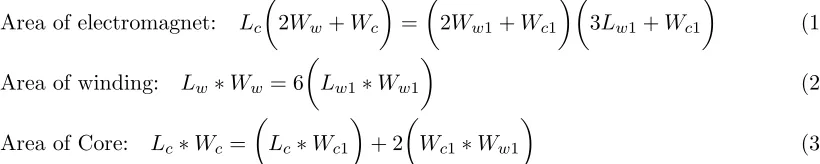
Figure 5. Half Halbach electromagnet. (a) Area considered for FE analysis. (b) Magnetic flux density. (c) 2D flux lines.
(a) (b) (c)
Figure 6. Full Halbach electromagnet. (a) Area considered for FE analysis. (b) Magnetic flux density. (c) 2D flux lines.
Also from Figure 5(c) it can be observed that the magnetic flux is only concentrated on one side (top) of the electromagnet.
The dimensions of electromagnet obtained by solving the Equations (1)–(4) for full Halbach arrangement are ‘Ww1 = 10.3 mm’, ‘Wc1= 4.4 mm’ and ‘Lw1 = 4.7 mm’. The developed electromagnet
of the required dimensions along with the different areas considered for FE analysis is shown in Figure 6(a), where (1), (3) and (5) show the horizontal electromagnet while (2) and (4) show the vertical electromagnet as shown in Figure 7(a). The magnetic flux density and 2D flux lines are plotted in Figures 6(b) and 6(c), respectively. The maximum value of flux density is observed to be 0.221 T, which is 1.8 times of the value of single electromagnet and 1.14 times of he half Halbach arrangement. From Figure 6(c) it is observed that in this configuration the magnetic flux is also only concentrated on one side (top) of the electromagnet.
Bottom side Top side
Reduction of flux
Reduction of flux
Reduction of flux Addiction of flux
Figure 7. Magnetic flux of half Halbach arrangement.
3. PARAMETRIC STUDY OF HALF HALBACH ARRANGEMENT
Before carrying out the parametric study on half Halbach arrangement, the magnetic field generated by each electromagnet is studied. The loop formed by each electromagnet is shown in Figure 7. From this figure, it can be observed that the magnetic field generated by the two horizontal electromagnets is added at the top side due to the same field direction, and the field gets reduced at the bottom side due to the opposite direction of field. To generate such an effect, the direction of winding at the bottom electromagnet has to be opposite to the winding direction with respect to top electromagnet as shown in Figure 8(a). The magnetic flux is generated by this arrangement plotted in Figure 8(b), and magnetic 2D flux lines are shown in Figure 8(c).
(a) (b) (c)
Figure 8. Modified half Halbach arrangement. (a) Modified half Halbach arrangement. (b) Magnetic flux density. (c) 2D flux line.
Parametric study was carried out by varying the ratio (0.75, 1.0, 1.25) of length of winding of horizontal electromagnet (Lw1) to vertical electromagnet (2Lw2) as depicted in Figure 3(c). The values
of magnetic flux densities for ratios 0.75 and 1.25 are shown in Figures 9(a) and 9(b), respectively. From the above discussion, following conclusion can be made:
Full Halbach arrangement generates higher magnetic flux density than the other two arrangements. The magnetic flux density value for full Halbach arrangement is 1.14 times of the half Halbach
(a) (b)
Figure 9. Magnetic flux density for different windings area in horizontal to vertical electromagnets. (a) 0.75. (b) 1.25.
Though the full Halbach arrangement provides better performing than the half Halbach arrangement, the manufacturing and providing windings in the core to get required arrangement is difficult and requires skilled labor.
For different values of winding ratio, the value of magnetic flux value is almost the same. Therefore, the total area of winding of three electromagnets is important rather than the ratio of winding in each electromagnet.
4. EXPERIMENTAL SETUP AND VALIDATION
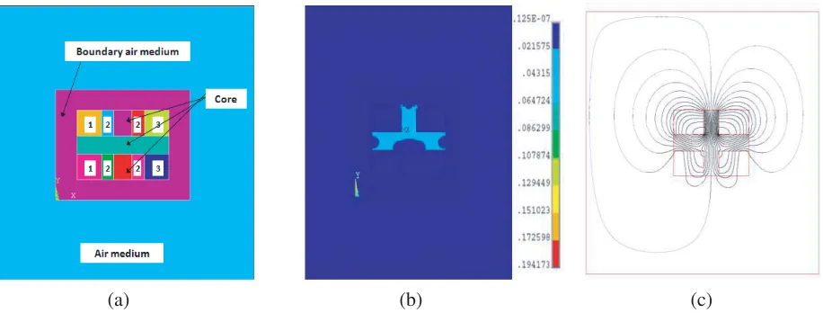
To validate the FE results obtained in previous heading, three half Halbach arrangements (as shown in Figure 10(a)) were fabricated. The length of the core (Lc) = 32.5 mm, width of the core (Wc1) = 6.5 mm
and axial Length of core = 30 mm were selected. Electromagnet with winding is shown in Figure 10(b), where the length (Lw1) and width (Ww1) of winding equal to 9.2 mm and 8.7 mm, respectively, were
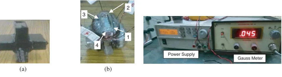
kept. Current to the electromagnet was supplied using a power supply (maximum current of 3 A and maximum voltage 24 V). The magnetic flux density was measured using the Gauss meter as shown in Figure 11. The magnetic flux density was measured at the four corners of the electromagnets as shown in Figure 10(b), and the results are listed in Table 1. From Figure 8(b), the magnetic flux density value estimated at the corners of the electromagnet after performing 2D FE analysis results is approximately 0.0475 T, and comparing this theoretical result with the tabulated results in Table 1 it can be concluded that the theoretical and experimental results are matching.
Table 1. Magnetic flux density value at different location.
Electromagnet Location 1 Location 2 Location 3 Location 4
1 0.045 0.042 0.048 0.046
2 0.046 0.046 0.046 0.044
3 0.046 0.048 0.043 0.045
The finite dimension of Gauss meter probe causes errors in angular measurement. In the present case, 4 mm width of the Gauss meter probe makes it very difficult to measure flux density at any location and results in error.
1 2 3
4
(a) (b)
Figure 10. Half Halbach arrangement. (a) Core. (b) Core with winding.
Power Supply
Gauss Meter
Figure 11. Power supply and Gauss meter.
single electromagnet arrangement. The aim of the present research is to reduce the supply current to the existing single electromagnet in order to reduce the running cost. 2D finite element analysis was performed again by reducing the supply current to the half back electromagnet till the magnetic flux density is equal to the single electromagnet. It was observed that for the magnetic flux value of 0.64 A the magnetic flux values of both arrangements yielded approximately the same value. For validating this results, the experiments were repeated by reducing the current and measuring the magnetic flux value at the corner of the electromagnets. It was observed that for current value of 0.69 A, the 2D finite element analysis and experiment results matched.
From the above discussion it can be concluded that by using the proposed half Halbach arrangement (having the same volume of normal electromagnet), to achieve the higher load carrying capacity, either the current supplied to the electromagnet can be reduced (i.e., reduction in the running cost of the Electromagnet) or the strength of the magnetic flux density can be increased.
5. CONCLUSION
To develop an electromagnet with high magnetic flux compared to a normal electromagnet, 2D finite element analysis was carried out on: (i) single electromagnet, (ii) half Halbach and (iii) full Halbach arrangements. Following conclusions were made:
Full Halbach arrangement generates higher magnetic flux density than the other two arrangements. The magnetic flux density value for full Halbach arrangement is higher than the half one.
Due to the complexity in developing full Halbach array arrangement, half Halbach arrangement was considered for further analysis.
Maximum magnetic flux in the half Halbach arrangement is obtained when the direction of magnetic flux is perpendicular to the adjacent electromagnet.
The parametric analysis on half Halbach arrangement showed that the ratio of winding in different electromagnets did not matter.
The value of the 2D finite analysis was verified with experimental results.
By using the proposed arrangement, the current required can be reduced by 31%.
REFERENCES
1. Betschon, F., “Design principles of integrated magnetic bearings,” PhD Thesis, 31–32, Swiss Federal Institute of Technology, 2000.
3. Noh, M. D., S. R. Cho, J. H. Kyung, S. K. Ro, and J. K. Park, “Design and implementation of a fault-tolerant magnetic bearing system for turbomolecular vacuum pump,”IEEE/ASME Trans. Mechatronics, Vol. 10, No. 6, 626–631, 2005.
4. Lijesh, K. P. and H. Hirani, “Optimization of eight pole radial active magnetic bearing,” ASME, Journal of Tribology, Vol. 137, No. 2, 2015, doi: 10.1115/1.4029073.
5. Nagaya, S., N. Kashima, M. Minami, H. Kawashima, and S. Unisuga, “Study on high temperature superconducting magnetic bearing for 10 kWh flywheel energy storage system,”IEEE Transactions on Applied Superconductivity, Vol. 11, No. 1, 1649–1652, 2001.
6. Lijesh, K. P. and H. Hirani, “Stiffness and damping coefficients for rubber mounted hybrid bearing,”
Lubrication Science, Vol. 26, No. 5, 301–314, 2014.
7. Hirani, H. and P. Samanta, “Hybrid (hydrodynamic + permanent magnetic) journal bearings,”
Proc. Inst. Mech. Eng., Part J, J. Eng. Tribol., Vol. 221, No. 8, 881–891, 2007.
8. Schweitzer, G., H. Bleuler, and A. Traxler, “Active magnetic bearing, basics, properties and applications of active magnetic bearing,” Vdf Hochschulverlag AG an der ETH, Zurich, 1994. 9. Williams, R. D., F. J. Keith, and P. E. Allaire, “Digital control of active magnetic bearings,”IEEE
Transactions on Industrial Electronics, Vol. 37, No. 1, 19–27, 1990.
10. Sahinkaya, M. N., A. H. G. Abulrub, P. S. Keogh, and C. R. Burrows, “Multiple sliding and rolling contact dynamics for a flexible rotor/magnetic bearing system,”IEEE/ASME Trans. Mechatronics, Vol. 12, No. 2, 179–189, 2007.
11. Noh, M. D., S. R. Cho, J. H. Kyung, S. K. Ro, and J. K. Park, “Design and implementation of a fault-tolerant magnetic bearing system for turbo molecular vacuum pump,” IEEE/ASME Trans. Mechatronics, Vol. 10, No. 6, 626–631, 2005.
12. Shankar, S., S. Sandeep, and H. Hirani, “Active magnetic bearing: A theoretical and experimental study,”Ind. J. Tribol., Vol. 1, 15–25, 2006.
13. Yonnet, J. P., G. Lemarquand, S. Hemmerlin, and E. Olivier-Rulliere, “Stacked structures of passive magnetic bearings,” J. Appl. Phys., Vol. 70, No. 10, 6633–6635, 1991.
14. Xu, F., L. Tiecai, Y. Liu, and H. Magnetization, “A study on passive magnetic bearing with Halbach magnetized array,” International Conference on Electrical Machines and Systems, 2008, ICEMS 2008, 417–420, 2008.
15. Fang, J., Y. Le, J. Sun, and K. Wang, “Analysis and design of passive magnetic bearing and damping system for high-speed compressor,” IEEE Transactions on Magnetics, Vol. 48, No. 9, 2528–2537, 2012.
16. Halbach, K., “Design of permanent multipole magnets with oriented rare earth cobalt material,”
Nuclear Instruments and Methods, Vol. 169, 1–10, 1980.
17. Mark, A. C., “Electric motor with Halbach arrays,” US 7598646 B2, 2007.
18. Gan, Z., X. Huang, H. Jiang, L. Tan, and J. Dong, “Analysis method to a Halbach PM ironless linear motor with trapezoid windings,” IEEE Transactions on Magnetics, Vol. 47, No. 10, 4167– 4170, 2011.
19. Edward, J. P., D. Stoikov, L. F. da Luz, and A. Suleman, “A performance evaluation of an automotive magnetorheological brake design with a sliding mode controller,”Mechatronics, Vol. 16, No. 7, 405–416, 2006.
20. Hartman, N. and R. A. Rimmer, “Electromagnetic, thermal, and structural analysis of RF cavities using ANSYS,”Proceedings of the 2001 Particle Accelerator Conference, 2001, PAC 2001, Vol. 2, 912–914, 2001.
21. Pilat, A., “FEMLab software applied to active magnetic bearing analysis,” International Journal of Applied Mathematics and Computer Science, Vol. 14, 497–501, 2004.