New Algorithm for Rain Cell Identification and
1
Tracking in Rainfall Event Analysis
2
Ting He 1,2,*, JianXin Zhang 1,*, JiYao Hua 1 and Yang Cai 1
3
1. Information Center (Hydrology Monitor and Forecast Center), Ministry of Water Resources, P.R. China,
4
No.2, Lane 2, BaiGuang Road, BeiJing 100053, China
5
2. Institute of Geographical Sciences, Free University of Berlin, Berlin, 12249, Germany
6
* Correspondence: [email protected], [email protected]
7
Abstract: This study proposes a new algorithm termed rain cell identification and tracking (RCIT)
8
to identify and track rain cells from high resolution weather radar data. Previous algorithms have
9
limitations when tracking non-consequent rain cells owing to their use of maximum correlation
10
coefficient methods and their lack of an alternative way to handle the variation stages of rain cells
11
during their life cycles. To address these deficiencies, various methods are implemented in the new
12
algorithm. These include the particle image velocimetry (PIV) method for motion estimation and
13
the rain cell matching rule to obtain the stage changes of rain cells. High resolution (5-min and
1-14
km) radar reflectivity data from three rainy days over the German federal state North Rhine
15
Westphalia (NRW) are used to evaluate the proposed algorithm. The performance of the new
16
algorithm is compared with a radar reflectivity map and verified by two object-oriented methods:
17
structure–amplitude–location (SAL) and geometric index. The verification results suggest that the
18
performance of the new algorithm is good. Application of the RCIT algorithm to the selected cases
19
shows that the inner structure of rainfall events in the experimental region present extreme value
20
distributions, with most rainfall events having a short duration with less intensity. The new
21
algorithm can effectively capture the stage changes of rain cells during their life cycles. The
22
proposed algorithm can serve as the basis for further hydro-meteorological applications such as
23
spatial and temporal analysis of rainfall events and short-term flood forecasting.
24
Keywords: rain cell; tracking; PIV; feature-based verification
25
1. Introduction
26
Precipitation is a key process in Earth’s water circle. Acquiring explicit knowledge about its
27
inner behavior is critical to assisting us in understanding its interaction with hydrological processes.
28
Rainfall events are characterized by several elements, such as duration, intensity, velocity, and spatial
29
and temporal variability (Elena et al. 2017). The variability of rainfall events can be defined as “the
30
variability derived from having multiple spatially-distributed rainfall fields for a given point in time”
31
(Peleg et al. 2017). In hydro-meteorological applications, rainfall always varies over its life cycle; this
32
variation also differs between different types of event (e.g., convective and stratiform rainfall events).
33
As a consequence, the responses of hydrology models are sensitive to this variation. Modeling rainfall
34
events and analyzing their spatial and temporal information is necessary.
35
For rainfall event monitoring, intensity and cumulative value are the two most common indexes
36
and they are usually measured using a rain gage, which is the standard instrument for providing
37
direct observations. Nevertheless, a rain gage cannot directly detect variability in rainfall events, it is
38
also subject to errors owing to topography and wind effects. As a possible alternative, weather radar
39
has played a major role in recent years owing to its high spatial and temporal resolution. This is
40
advantageous in terms of (i) acquiring spatial and temporal patterns when modeling rainfall events
41
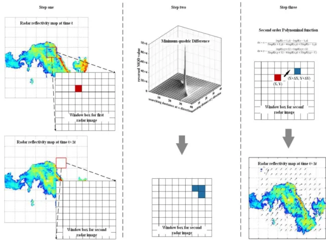
and (ii) undertaking short-term rainfall forecasting at fine scales. Identifying and tracking rainfall
42
events is a common task in radar-based meteorological and hydrological applications (Moseley et al.
43
2013; Novo et al. 2014; Guinard et al. 2015; Yeung et al. 2015).
44
Broadly speaking, the corresponding algorithms for radar-based rainfall event identification and
45
tracking can be classified into and object-based approaches (Zahraei et al. 2013). The
pixel-46
based approaches are also referred to as advection field tracking. These are pattern matching
47
approaches for extracting motion vectors by searching for the maximum correlation coefficient of
48
rain cells in two consecutive radar images. Pixel-based algorithms are highly effective when they are
49
applied in convective rainfall nowcasting, which is usually found in frontal systems (Anna et al.
50
2018). Algorithms of this kind are capable of distinguishing between large scale convective and
51
stratiform rainfall, although they are not so effective for individual RCIT. Herein, a rain cell is defined
52
as the closed contours over which rainfall intensity exceeds a given threshold during one rainfall
53
event (Féral et al. 2006). Representative algorithms can be listed as follows: TREC (Rinenart and
54
Garvey 1978), TITAN (Dixon and Wiener 1993), COTREC (Li et al.1995), and SWIRLS (Li et al. 2014).
55
Object-based approaches (also termed cell tracking) include (i) a detecting algorithm for searching a
56
discrete rain cell’s properties (e.g., centroid, area, echo-tops, and vertical-integrated) in consecutive
57
radar images and (ii) a matching algorithm for tracking cell motion and shape changes (e.g., merging
58
and splitting). The advantage of object-based approaches is in reflecting the dynamic of convective
59
rainfall; they are suitable for convective rain storm analysis but not effective in straitiform rainfall
60
identification. Representative algorithms can be listed as follows: SCOUT (Einfalt et al. 1990), SCIT
61
(Johnson et al. 1998), Trace3D (Handwerker 2002), and PERsiann-ForeCAST (Zahrani et al. 2013).
62
Despite the thorough application of these rain event identification and tracking algorithms, they
63
have the following deficiencies. For pixel-based approaches, motion estimates are mostly based on
64
the maximum correlation coefficient, which may yield non-continuous results when fast decay of
65
rainfall occurs. For object-based approaches, motion estimates obtained from the rain cell center of
66
mass may lack accuracy owing to the random center of mass displacement problem (Han et al., 2009).
67
This problem occurs when the shape of rain cells changes rapidly between successive radar images.
68
As a consequence of these motion estimate inaccuracies, these algorithms may also encounter
69
difficulties when handling merging and splitting scenarios (Muñoz et al., 2018), whereas a rain cell
70
can begin its life cycle by simply emerging at a location with no rain. It is also possible that a rain cell
71
can become separated from a large single rain cell or that several smaller rain cells can merge into
72
one (Moseley et al. 2013). For such reasons, a new rain cell identification and tracking algorithm
73
(RCIT) is proposed in this work. The algorithm is developed by combining the advantages of pixel-
74
and object-based approaches and is able to handle the problem of detecting the stage changes of rain
75
cells.
76
This paper is organized as follows. An introduction to the study area and radar data is given in
77
Section 2. The RCIT algorithm is illustrated in Section 3. Section 4 presents structure, amplitude, and
78
location (SAL) and geometric verification results and practical applications of the algorithm to North
79
Rhine Westphalia (NRW) rainfall events. In Section 5, the main conclusions and further expectations
80
of this work are given.
81
2. Rain Cell Identification and Tracking Algorithm - RCIT
82
The aim of the RCIT is to analyze rainfall events by fully utilizing the merits of weather radar.
83
The inputs to the proposed algorithm are radar reflectivity maps and the outputs are the properties
84
of rain cells such as area, intensity, and trajectory. The RCIT involves two modules: rain cell
85
identification and tracking, as presented as in Figure 1.
87
Figure 1. Step illustration of rain cell identification and tracking algorithm.
88
2.1. Rain Cell Identification Module
89
Similar to the object-based algorithms, the rain cell identification module of the RCIT is based
90
on discerning a connected domain above a given threshold. As presented in the left portion of Figure
91
1, each selected radar reflectivity map in the Cartesian coordinates is initially filtered by the median
92
filtering method (Anoraganingrum 1999) to remove noisy pixels (pixels with abnormally high
93
reflectivity). Then, pixels above a given reflectivity threshold are assigned the value one, with the
94
remainder assigned the value zero. A segmenting process is implemented to assemble and cluster
95
pixels sharing the same reflectivity threshold into a connected area. In the segmenting process, the
96
following rules suggested by Peleg and Morin (2012) are obeyed: (i) If the reflectivity of a rainy pixel
97
is lower than a given threshold Rt, then it is set to null. (ii) For each rainy pixel and its eight neighbors,
98
if more than five of them are null, then it is set to null. (iii) If the pixel is spurred, then it is set to null.
99
Herein, spur pixels are those isolated pixels whose reflectivity is different to others along the
100
horizontal and vertical directions in the labeled binary image. (iv) If the area of a connected region is
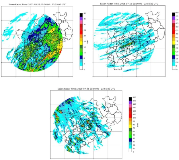
101
smaller than 9 km2, then it is ignored. All the segmented regions are then labeled and fitted with an
102
ellipse shape. Their properties are extracted and stored in a relational database. The extracted
103
properties are as follows:
104
i) Area [km2] - Sum value for the number of pixels contained in one rain cell.
105
ii) Areal rainfall depth [mm] - Cumulative precipitation of one rain cell over a 5-minute interval.
iii) Maximum intensity [mm.h−1] - Peak intensity of one rain cell.
107
iv) Areal mean rainfall depth [mm.km2] - Ratio of the areal rainfall depth and area.
108
v) Eccentricity - Ratio of minor and major axes, which are acquired from the fitted eclipse. Used
109
to describe the shape of one rain cell with a value range from 0 to 1.
110
vi) Center of mass [km] - Center of mass of a rain cell, which is weighted by the reflectivity of rainy
111
pixels.
112
Property calculation: Areal rainfall depth, maximum intensity, and areal mean rainfall depth are
113
based on the reflectivity (Z) and rain rate (R) converting function: Z = aRb.
114
2.2. Rain Cell Tracking Module
115
The rain cell tracking module is established based on a hybrid approach, as illustrated in the
116
right portion of Figure 1. In the first procedure, motion vectors are estimated by implementing the
117
particle image velocimetry (PIV). This is an optical method of flow visualization that is used to obtain
118
instantaneous velocity measurements and related properties of fluids (Merzkirch 2001; Adrian 2005;
119
Westerweel et al. 2013). It consists of a class of flow measuring mechanisms that are characterized by
120
recording the displacement of small particles embedded in a region of fluid. Figure 2 shows a PIV
121
application in motion vector estimation. In the first step, a window box of size r × r is initially defined,
122
which divides radar images into several sub-blocks. In the second step, a searching distance, d =
123
2 × v + 1, is defined, where vmax is the preset maximum velocity. The minimum quadric difference
124
(MQD), as suggested by Gui and Merzkirch (1996), is employed in searching the optimal grid points
125
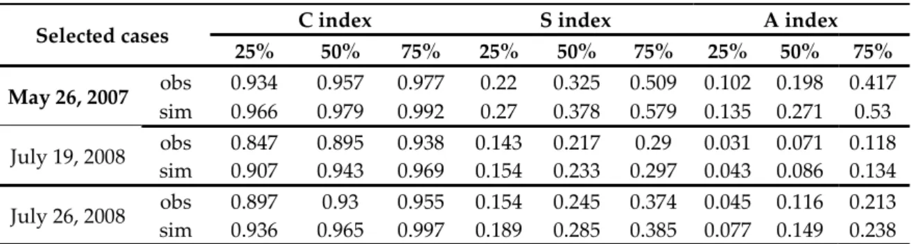
at time t + ∆t, as in Equation (1):
126
𝑀𝑄𝐷(Δ𝑥, Δ𝑦) = ∑ ∑ 𝑅 𝑋 , 𝑌 − 𝑅 𝑋 + Δ𝑥, 𝑌 + Δ𝑦 (1)
127
where R1(Xi,Yj)and R2(Xi,Yj) are the reflectivity of grid points contained within the window boxes of
128
radar images at time t and t+∆t, respectively; ∆x and ∆y (∆x,∆y ϵ d) are the locations of minimum
129
reflectivity difference in the horizontal and vertical directions separately. The minimum reflectivity
130
differences of grid points within the window boxes are reversed to simplify the calculation. In order
131
to guarantee that the solitary peak locations can be calculated, ∆x and ∆y are corrected separately in
132
the horizontal and vertical directions by fitting a second-order polynomial to the logarithm of the
133
maximum reflectivity of the grid point and its three direct neighbors, as in Equation (2). In this way,
134
the optimal grid points at time t + ∆t are identified, with their locations presented as (x + ∆x − , y +
135
∆y − ). In the final step, the calculated motion vectors are smoothed by the median filter algorithm.
136
∆𝑥 = 𝑥 − ( , ) ( , )
( , ) ( , ) ( , ) (2a)
137
∆𝑦 = 𝑦 − ( , ) ( , )
( , ) ( , ) ( , ) (2b)
138
In the second procedure, rain cells at time t and t + ∆t are identified. Finally, a child rain cell
139
matching rule is applied for identifying the most-matched rain cells. The child rain cell matching
140
scheme considers the stage changes of rain cells between successive radar images (e.g., merge, split,
141
growth, and decay), using certain indexes for determination such as overlap, area diversification,
142
distance, and angle difference of center of mass. Before introduction of the rain cluster matching rule,
143
certain definitions were identified: (i) for two radar images at time t and t + ∆t, rain cells identified
144
from radar images at t are termed parent cells and (ii) rain cells identified from radar images at t + ∆t
145
are termed child cells. These definitions can be depicted as follows:
(1) A boundary box of a parent cell is defined, with a horizontal length of [10+max(posx),
147
min(posx)−10] and vertical length of [10+max(posy), min(posy)−10], where posx and posy are
148
Cartesian coordinates of pixels in the parent cell.
149
(2) The number of child cells falling into the boundary box is determined and their
150
properties, e.g., area, areal rainfall depth, max intensity, areal mean rainfall depth, and
151
center of mass, are selected.
152
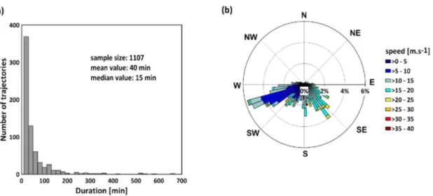
(3) If only one child cellis searched in the boundary box and it overlaps with a parent
153
cell, then it is the most-matched rain cell. If this child cell does not overlap with a parent cell
154
and the distance and angle difference for the center of mass between it and the parent cell
155
are less than 3 × mean (Vmotion_vector) and 3 × θmotion_vector, it is also the most-matched rain cell,
156
where mean (Vmotion_vector) and θmotion_vector are the mean value of velocity and the prevailing
157
direction of the motion vector, respectively.
158
(4) If two or more child cells fall into the boundary box without overlapping a parent cell,
159
the matching rule is changeless; however one extra condition is included, i.e., child cells
160
whose areas have minimum absolute differences with the parent cell are the most-matched
161
rain cells.
162
163
Figure 2. Illustration of PIV application in rain cell motion estimation. Step one: window boxes with
164
the area of r × r are defined (rectangular with red color); step two: for any grid point in the window
165
box at a previous timepoint (red block), the MQD algorithm is applied to deduce the minimum
166
reflectivity differences, and grid points with minimum value in the next window box are identified
167
(blue blocks); step three: the solitary locations of reversed MQD value, ∆x and ∆y, are corrected by
168
applying Equation (2). The locations of the optimal grid point at the next timepoint are calculated
169
using the second polynomial function, and the global motion vectors are extracted and smoothed by
170
the median filter method.
171
3. Study Area and Data
The study area is the federal state of NRW (Figure 3). It is bordered by the German federal states
173
of Lower Saxony to the north and north-east, Hessen to the east, and Rhineland–Palatinate to the
174
south, and by the countries of Belgium to the south-west and the Netherlands to the west. NRW
175
includes upland regions of North Eifel in the south and mountains of the Sauerland in the south-east.
176
There are five rivers in this study area: Rhine, Ruhr, Ems, Lippe, and Weser. Two main types of
177
landscape can be found in NRW, namely the North German lowlands, with elevations just a few
178
meters above sea level, and the North German low mountain range, with elevations of up to 850 m.
179
The lowland areas comprise the Rhine–Ruhr area, which is one of the largest metropolitan areas, with
180
a population of approximately 10 million. The circulation pattern of NRW is mainly affected by the
181
air mass from the Atlantic Ocean along the direction toward the mainland. When arriving at the
182
southern high mountain regions, the air mass stops and rises; this leads to more cloudiness and
183
precipitation. On the eastern side of the mountain regions, drier air masses result in less cloudiness
184
and less precipitation.
185
Radar data were obtained from the Essen radar deployed in Essen City, NRW. The Essen radar
186
has been deployed over the study area and is a part of the radar network of the German weather
187
service (DWD). The Essen radar is a dual-polarimetric C-band Doppler radar. It delivers radar
188
volume scans (frequency: 800/1200 Hz, maximum range: 124 km) every 15 minutes for the Doppler
189
velocity, together with intensity volume scans (frequency: 500 Hz, maximum range: 256 km) and
190
precipitation scans (frequency: 600 Hz, maximum range: 150 km) every 5 minutes for the
191
precipitation echo, with a high spatial resolution of 1 km in range and 1° in azimuth. For this study,
192
the Essen radar provided precipitation scans with an elevation of 0.8° and a range of 128 km. The
193
output reflectivity was selected with a plan position indicator (PPI) display type.
194
As radar measures precipitation in an indirect manner, the quality of radar data must be
195
carefully checked. The sources that affect the quality of the Essen radar data include ground clutter
196
and speckle, beam blockage, and attenuation. The corresponding quality correction methods in this
197
work follow Golz et al. (2006). After quality checking, an open source package “Wradlib”
198
(Heistermann et al. 2013) was applied to project the raw radar image onto a 256 × 256 km2 Cartesian
199
map with 1-km resolution. In total, 864 radar reflectivity images for three rainy days (May 26, 2007;
200
July 19, 2008; and July 26, 2008), including some recorded convective rainfall events, were selected to
201
evaluate the proposed algorithm. The daily rainfall distributions of these rainy days are shown in
202
Figure 4.
204
Figure 3. Study area of North Rhine Westphalia (NRW) and its location in Germany. The main
205
administrative cities are marked with red dots.
207
Figure 4. Daily rainfall distribution for selected rainy days. Radar reflectivity was converted into rain
208
rate according to DWD standard Z–R relationship.
209
4. Results Analysis and Discussion
210
In the algorithm application process, the reflectivity threshold for rain cell identification was set
211
to 19 dBZ, which was based on the classification of DWD presented by Weusthoff and Hauf (2008),
212
as in Table 1. For the German weather radar system, two common Z–R relationships were used by
213
Weusthoff and Hauf (2008): one was categorized for the RADOLAN product and the other uses
214
constant a and b with values of 256 and 1.42, respectively. Although the DWD has stated that the
215
categorized relationship statistically shows better results over long time periods, the standard
216
relationship can be more compatible with local cases when a correction factor is added (Einfalt and
217
Frerk 2012). Based on the above considerations, we applied the DWD standard Z–R relationship to
218
radar reflectivity–rain rate conversion in the application cases.
219
Table 1. Conversion of radar reflectivity to rain rates using Z–R relationship (a = 256, b = 1.42) with
220
thresholds according to the classification of the DWD.
221
Z [dBZ] R [mm.h−1] Rain Rate [mm.5 min−1]
4.1. Performance Assessment of RCIT Algorithm
222
Grid-point related error measurement is problematic for the rain cell tracking algorithm. A
223
classic example illustrating this problem is the well-known “Double Penalty” problem, in which
224
prediction of a precipitation object at the correct size and structure might yield very poor verification
225
scores. For example, one rain cell is displaced slightly in space but the categorical verification scores
226
heavily penalize such a situation. In traditional verification methods, a displacement simply leads to
227
a false alarm, and it is also very poorly rated owing to its large root mean squared error (Davis et al.
228
2006). On the other hand, despite a great deal of effort in the statistical validation of grid-based
229
rainfall estimated results, verification associated with the geometry patterns of rain cells has not been
230
well researched or applied.
231
As an alternative, feature-based verification methods have been built upon the idea of
232
identifying rainfall events as “objects”. With this perspective, simulated and observed rainfalls are
233
not compared directly at the same location; rather, objects of interest are extracted from simulated
234
and observed data and then compared together so that verification statistics are obtained. A number
235
of spatial verification methods have been proposed (Ebert 2008; Gilleland et al. 2009). In the present
236
work two feature-based verification methods, SAL and geometric index, are implemented to verify
237
the performance of the RCIT algorithm. A detailed introduction to the SAL and geometric index
238
methods is presented in Appendix A. The data set for comparison was a simulated radar reflectivity
239
map from the RCIT algorithm (termed sim_ref) and an observed radar reflectivity map (termed
240
obs_ref).
241
Figure 5 shows the SAL verification results, which are arranged based on the three selected rainy
242
days. For each SAL plot presented in Figure 5, the vertical axis denotes the A component, the
243
horizontal axis denoted the S component, the dots represent values of the S and A components, and
244
the color scale of the dots denotes the L component. Median values of the SAL components are
245
presented as dashed lines. It can be seen that all S and A values are concentrated close to zero, as are
246
most L component values. Table 2 gives the S, A, and L index values for the geometric index objects
247
from the sim_ref and obs_ref data sets. All values were again organized based on the three selected
248
rainy days. It is evident that the index differences between the geometric index objects from the
249
sim_ref and obs_ref data sets were less than 0.05.
250
Table 2. Results of three geometric index components of geometric index verification objects for
RCIT-251
simulated radar reflectivity maps (sim) and observed radar reflectivity maps (obs). Values are sorted
252
at 5, 50, and 75 percentile levels.
253
Selected cases C index S index A index
25% 50% 75% 25% 50% 75% 25% 50% 75%
May 26, 2007 sim obs 0.934 0.966 0.957 0.979 0.977 0.992 0.22 0.27 0.325 0.509 0.102 0.198 0.417 0.378 0.579 0.135 0.271 0.53
July 19, 2008 sim obs 0.847 0.907 0.895 0.943 0.938 0.143 0.217 0.969 0.154 0.233 0.297 0.043 0.086 0.134 0.29 0.031 0.071 0.118
July 26, 2008 sim obs 0.897 0.936 0.965 0.93 0.955 0.154 0.245 0.374 0.045 0.116 0.213 0.997 0.189 0.285 0.385 0.077 0.149 0.238 The SAL verification results suggest that the shape of most SAL objects from the sim_ref data
254
set was the same as that for SAL objects from the obs_ref data set (except for a few cases that were
255
slightly large and flat). The converted rainfall volume for some SAL objects from the sim_ref data set
256
was less than that from the obs_ref data set; the origin that the rain cell area threshold used in the
257
RCIT algorithm was 9 km2, with rain cells less than this threshold ignored. However, the converted
258
rainfall volume of most SAL objects from the sim_ref data set was close to that from the obs_ref data
259
set. Location differences of SAL objects between the sim_ref and obs_ref data sets were not obvious.
260
Geometric index verification results indicated that the geometric pattern of geometric index objects
261
from the sim_ref data set was approximately the same as that for objects from the obs_ref data set
262
(except for connectivity). Differences in the C index for geometric index objects from the two data
sets were obvious, which may have been because the median filter method applied in the RCIT
264
algorithm smoothed abnormal pixels in the radar reflectivity map. In general, the RCIT algorithm
265
performed well based on the two feature-based verification methods.
266
267
Figure 5. Value distributions of the three SAL components. Dashed lines in the vertical and horizontal
268
directions in each sub-figure represent the median values of the S and A components, respectively,
269
and dot color represents the of L component value. Results are sorted by selected rain days: (a) May
270
26, 2007; (b) July 19, 2008; (c) July 26, 2008.
271
4.2. Application of RCIT Algorithm in Rainfall Event Analysis
272
There were 10,346 rain cells identified from the radar reflectivity maps. Descriptive statistics of
273
their properties are given in Table 3. It was found that a high standard deviation existed for the areas
274
of these rain cells, with values ranging from 9 to 18,734 km2 (most were less than 38 km2). For areal
275
rainfall depth, values ranged from 0.36 to 8861 mm and a high standard deviation again existed. For
276
the maximum intensity property, a high standard deviation (34.08 mm.h−1) was also found; the
277
median value was 2.83 mm.h−1 and the range of values was 0.48 to 397.75 mm.h−1. Areal mean rainfall
278
depth was from 0.04 to 4.4 mm.km2. Eccentricity ranged from 0 to 1, with a median value over 0.5.
279
Table 3. Descriptive statistics of rain cell properties. Indexes used for the statistics are minimum
280
value, maximum value, standard deviation, and median value.
281
Property
Statistical properties
Minimum value
Maximum value
Standard deviation
Median value
Area 9 18734 1391 38
Areal rainfall depth 0.36 8861 559.9 4.4
Max intensity 0.04 33.2 2.8 0.24
Areal mean rainfall
depth 0.04 4.4 0.3 0.1
Eccentricity 0 0.99 0.17 0.84
Inner structures of the selected events were described by statistically analyzing the physical and
283
geometric properties of the rain cells. RCIT simulation results indicated that the properties (e.g., area,
284
areal rainfall depth, max intensity, and areal mean rainfall depth) of the identified rain cells presented
285
a wide range of values. The shape of the rain cells was somewhat elliptical, with a median value over
286
0.5. Histograms of the log10-transformed rain cell properties are given as in Figure 6. To determine
287
the best theoretical distributions describing the empirical distributions, a multi-goodness of fit testing
288
(GOF) approach combined with the Akaike information criterion (AIC), the Bayesian information
289
criterion (BIC), and the Kolmogorov–Smirnov (K–S) test methods was applied (see Appendix B).
290
Figure 7 shows their fitted cumulative distributions. Empirical distributions of the log10-transformed
291
properties (area, areal rainfall depth, maximum intensity, and areal mean rainfall depth) could be
292
fitted with the generalized Pareto distribution (GPD) presented in Equation (6), and the extreme
293
value distribution (EVD) was found to fit the eccentricity property shown in Equation (7).
294
f(x|k, μ, α) = ( )(1 + k
( ))
(6)
295
where k is the shape parameter, and μ and α are location and scale parameters, respectively. For
296
μ < 0, k is above zero, and for μ < x < α, k is below zero. At the limit for k = 0, the GPD is the
297
exponential distribution.
298
f(x|k, μ, α) = ( )e
( ( ( )) )( ( ))(7)
299
for 1 + k( αμ), when k > 0, the generalized EVD is the Frchet distribution; k < 0 corresponds to the
300
Weibull distribution; at the limit for k = 0, it is the Gumbel distribution.
301
A total of 1,107 rain cell trajectories were exploited. Histograms of their duration and motion
302
vectors are presented in Figure 8. All rain cells held a mean duration of 40 minutes. For all the
303
identified rain cells, the median value of their life cycles was 15 minutes, with an average moving
304
speed of 11.59 m.s−1. The moving directions of the rain cells were consistently toward the direction of
305
motion observed in the radar images.
306
Figure 6. Histograms of log10-transformed rain cell properties: (a) area, (b) areal rainfall depth, (c)
308
maximum intensity, (d) areal mean rainfall depth and property, (e) eccentricity for identified rain
309
fields.
310
311
Figure 7. Cumulative curves of fitted probability density functions for log10-transformed rain cell
312
properties: (a) area, (b) areal rainfall depth, (c) maximum intensity, (d) areal mean rainfall depth and
313
property, (e) eccentricity.
314
315
Figure 8. (a) Histograms of rain cell duration for identified rain fields, (b) wind rose plot of rain cell
316
motion estimation result.
317
These results were in agreement with the study of Barnolas et al. (2010), in which the structures
318
of heavy rainfall events recorded in Catalonia, Spain were analyzed. However, the results differed
319
from those of Karklinsky and Morin (2006), in which the area of identified rain cells in southern Israel
320
was better fitted to the log-normal distribution. Statistical analysis of the rain cell properties suggests
321
that the inner structures of the selected rainy days can be expressed by the EVD. This suggests that
322
most rainfall events had a limited covering area with less intensity and short duration; rainfall events
323
with a long duration had a large covering area and high intensity.
During the life cycle of a rainfall event, the physical and geometrical features of rain cells
325
continually change. Three common stages reflect these variations: cumulus, mature, and dissipating
326
(Byers and Braham Jr 1948). In fact, the stage changes of rain cells are not only associated with its
327
internal growth and decay but also with outer rain cells (e.g., merging or splitting). In this study,
328
seven rain cell life stages were confirmed by the RCIT algorithm; their definitions can be listed as
329
follows (Figure 9):
330
a. Initial: A rain cell having no parent cell is termed an initial rain cell.
331
b. Tracking: A rain cell with only one parent cell and having no interaction with other rain
332
cells during its life cycle is termed a tracking rain cell.
333
c. Merge: A rain cell with at least two parent cells is termed a merged rain cell.
334
d. Split: A rain cell with only one parent cell but at least two child cells is termed a split rain
335
cell.
336
e. Dissipate: A rain cell with at least one parent cell but no child cells is termed a dissipate
337
rain cell.
338
f. 5-minute life cycle: A rain cell with a life cycle of only 5 minutes.
339
g. Complex stage: A rain cell for which merging and splitting simultaneously exist during its
340
life cycle is termed complex stage.
341
The number of rain cells with different stages over their life cycles is summarized in Table 4.
342
Rain cells with “5 minutes life cycle” and “tracking” stages were dominant. The “merging”,
343
“splitting”, and “complex stage” cells occurred in isolated cases, indicating a stable inner structure
344
of the identified cells. For the cases of July 19, 2008 and July 26, 2008, the number of rain cells in the
345
“tracking” stage was even greater, indicating that the rainfall events occurring on these two days had
346
long durations. The number of rain cells in the “merging” and “splitting” stages was greater in the
347
July 26, 2008 case. This suggests that there were more convective rainfall events on that day since rain
348
cells merge or split more frequently under such conditions.
349
Table 4. Number of rain cells with different life stages, sorted by selected rain day.
350
Stages May 26, 2007 July 19, 2008 July 26, 2008
Initial 158 350 471
Tracking 608 1270 1787
Merge 7 6 39
Split 1 2 5
Dissipate 152 346 434
5 minute life cycle 632 3148 929
Complex stage 0 0 1
352
Figure 9. Stage definitions of rain cells: (a) initial, (b) tracking, (c) merging, (d) splitting, (e)
353
dissipating.
354
5. Conclusion and Outlook
355
This study develops a new algorithm, RCIT, which utilizes the advantages of high resolution
356
weather radar data. The proposed algorithm provides the following improvements:
357
1. It uses the PIV method in rain cell motion estimation. Rain cell motion estimation by past
358
algorithms is mainly based on the maximum correlation coefficient method, which may
359
lead to nonconsecutive motion when the shape and volume of a rain cell change rapidly.
360
The PIV method avoids this situation.
361
2. A rain cell matching rule is proposed to discern the life cycle and stage change of rain cells.
362
Past algorithms focus mainly on the tracking of rain cells without merging and splitting,
363
when in fact rain cell stage variation is obvious over their life cycle, especially for
364
convective rainfall events. The proposed rain cell matching rule implemented in the RCIT
365
algorithm can easily and effectively discern the various stages of rain cells.
366
Two feature-based verification methods, SAL and geometric index, were used to test the
367
performance of the RCIT algorithm. It is shown that all verification indexes fall within in a reasonable
368
error range, confirming the good performance of the RCIT algorithm. Practical applications of the
369
RCIT algorithm in analyzing the inner structure of historical rainfall events that occurred in the NRW
370
are presented. This is the first time that the use of such a RCIT algorithm to depict the inner structures
371
of rainfall events in an urban region with a high population density has been presented. The results
372
show that the properties of rain cells in this region presented an EVD, indicating that the selected
373
rainfall events had a short duration with low intensity. Long duration events with high intensity are
374
rarely found and the stage changes of rain cells vary between events.
375
It should be noted that inputs for the proposed algorithm is not limited to radar data; other 2-D
376
remote sensing data will also be used as the algorithm inputs, suggesting the versatility of the
proposed algorithm. In future application, it is intended that this algorithm will analyze the spatial–
378
temporal variation of rainfall in small regions; this will lead to the determination of rainfall inputs
379
with proper spatial and temporal scales for hydro-meteorological applications. The proposed
380
algorithm will also be applied to rainfall nowcasting, which will improve the foresight period of flash
381
floods in mountainous and urban regions. In addition, the features of the rain cell output from this
382
algorithm can be used in sensitivity analyses of urban runoff in relation to short-term rainfall events,
383
which will improve flood forecasting precision in small–medium catchments.
384
Acknowledgments: Authors would like to thank WUPPERVERBAND (water management in
385
Wupper area) for radar data support and to thank Dr. Thomas Einfalt from Hydro&Meteoro Co Ltd
386
for the guidance about radar data quality control. The financial support for this study was made
387
available by the International Science & Technology Cooperation Program of China (Grant No:
388
2012DFG22140).
389
APPENDIX A
390
Structure–Amplitude–Location (SAL) and Geometric Index Verification Methods
391
Two feature-based verification methods, structure–amplitude–location (SAL) and geometric
392
index, were applied to evaluate the performance of the RCIT algorithm and nowcasting methods. In
393
SAL, term structure denotes the similarity in the shapes of modeled and observed rain cells; its value
394
range is from −2 to 2. Amplitude denotes the similarity in the total precipitation values of modeled
395
and observed rain cells; its value range is from −2 to 2. Location denotes the similarity of the center
396
of mass for the modeled and observed rain cells; its value varies from 0 to 2. The accuracy of
397
nowcasting methods can be evaluated based on the value of the three SAL components and a perfect
398
nowcasting is confirmed by S, A, and L values of 0. More details on the SAL method can be found in
399
Wernli et al. (2008).
400
Geometric index is a quantitative assessment method for the spatial patterns of rain cells
401
(AghaKouchak et al. 2010). It compares the geometric features of modeled and observed rain cells via
402
three indexes:
403
Connectivity index: This is defined to compare simulated rain cells with respect to a
404
reference object (e.g., observed rain cells). Its value is calculated based on the number of
405
rain cells (NC) and the total number of non-zero pixels or pixels above a given threshold
406
(NP), as in Equation (8):
407
𝐶 = 1 −
√ (8)
408
where Cindex is the connectivity index, NP is the number of rainy pixels above a given
409
threshold, and NC is the number of rain cells.
410
Shape index: This index is introduced to quantitatively describe the shape discrepancy of
411
rain cells, as in Equation (9):
412
𝑆 = 1 − (9)
413
where Sindex is the single index, Pmin is the theoretical minimum perimeter, and P is the
414
actual perimeter of the rain cell.
Area index: This is defined to depict the dispersiveness between the modeled and
416
observed rain cells. Its value is the ratio of the area of its convex hull (the boundary of the
417
minimal convex set containing a finite set of points in the rain cell), as in Equation (10).
418
𝐴 = 1 − (10)
419
where A is the area of the rain cell and AConvex is the area of the convex hull.
420
APPENDIX B
421
Goodness of fit testing for fitted distributions of rain cell properties
422
The GOF test determines whether a data set is well fitted with a predefined distribution that
423
gives the highest probability of producing the observed data. As such, a series of fit testing methods
424
was developed, with the commonly applied tests as follows:
425
The K–S test is based on the empirical cumulative distribution function (ECDF). Given N
426
ordered data points Y1, Y2, …., Yn, their ECDF is defined as:
427
𝐸 = ( ) (11)
428
where n(i) is the number of points less than Yi and Yj, which are ordered from the smallest
429
to largest value. This is a step function that increases by 1/N at the value of each ordered
430
data point. The K–S test was developed according to the following hypotheses: H0—the
431
data follow a specified distribution; H1—the data do not follow the specified distribution.
432
AIC (Akaike, 1998) is based on the use of Kullback–Leible information as the discrepancy
433
measure between the true distribution and the approximating distributions: Mi =
434
gi(x,p1,p2,…,pn). The AIC for the ith candidate distribution can be computed as:
435
𝐴𝐼𝐶 = −2 ∏(𝜃) + 2𝑝 (12)
436
where ∏(θ) stands for the maximum log-likelihood of the sample of the dataset, p is the
437
parameter’s number of candidate distributions when the sample size n is small with
438
respect to the number of the estimated parameter Pi. The smaller the value of AIC, the
439
better fitting is the result for the candidate distribution.
440
BIC (Schwarz, 1978) serves as an asymptotic approximation to a transformation of the
441
Bayesian posterior probability of a candidate model. It is based on the empirical
log-442
likelihood and does not require the specification of priors. BIC is defined as
443
𝐵𝐼𝐶 = −2 ∏(𝜃) + ln (𝑛)𝑝 (13)
444
where the symbols are the same as those In Equation (12). A small value of BIC means
445
that the candidate distribution fits well with the empirical distribution.
References
447
Adrian R. 2005. Twenty years of particle image velocimetry. Exp Fluids, 39: 159–169
448
AghaKouchak A, Nasrollahi N, Li J, Imam B, Sorooshian S. 2010. Geometrical characterization of
449
precipitation patterns. J Hydrometeorol, 12: 274–285
450
Akaike H. 1998. Information theory and an extension of the maximum likelihood principle. In: Parzen
451
E, Tanabe K, Kitagawa G, eds. Selected Papers of Hirotugu
452
Akaike. Springer New York. Springer Series in Statistics, 199–213
453
Anna D M, Tomeu R, Carmen L M. 2018. A radar-based centroid tracking algorithm for severe
454
weather surveillance: Identifying split/merge processes in convective systems. Atmos Res, 213: 110–
455
120
456
Anoraganingrum D. 1999. Cell segmentation with median filter and mathematical morphology
457
operation, in: Image Analysis and Processing. 1999. Proceedings. International Conference on Image
458
Analysis & Processing. 1043–1046
459
Barnolas M, Rigo T, Llasat M C. 2010. Characteristics of 2-d convective structures in catalonia (ne
460
spain): An analysis using radar data and gis. Hydrol Earth Syst Sci, 14: 129–139
461
Casati B, Wilson L J, Stephenson D B, Nurmi P, Ghelli A, Pocernich M, Damrath U, Ebert E E, Brown
462
B G, Mason S. 2008. Forecast verification: Current status and future directions. Meteorol Appl, 15: 3–
463
18
464
Davis C, Brown B, Bullock R. 2006. Object-based verification of precipitation forecasts. Part I:
465
Methodology and application to mesoscale rain areas. Mon Weather Rev, 134: 1772–1784
466
Dixon M, Wiener G. 1993. Titan: Thunderstorm identification, tracking, analysis, and nowcasting—
467
A radar-based methodology. J Atmospheric Ocean Technol, 10: 785–797
468
Ebert E, Wilson L, Weigel A, Mittermaier M, Nurmi P, Gill P, Gober M, Joslyn S, Brown B, Fowler T,
469
Watkins A. 2013. Progress and challenges in forecast verification. Meteorol Appl, 20: 130–139
470
Ebert E E. 2008. Fuzzy verification of high-resolution gridded forecasts: A review and proposed
471
framework. Meteorol Appl, 15: 51–64
472
Einfalt T, Denoeux T, Jacquet G. 1990. A radar rainfall forecasting method designed for hydrological
473
purposes. J Hydrol, 114: 229–244
474
Elena C, Marie-Claire T V, Nick V D G. 2017. Spatial and temporal variability of rainfall and their
475
effects on hydrological response in urban areas—a review. Hydrol Earth Syst Sci, 21: 3859–3878
476
Féral, Laurent, Sauvageot H, Castanet L, Lemorton J, Cornet, Frédéric, Leconte K. 2006. Large-scale
477
modeling of rain fields from a rain cell deterministic model. Radio Sci, 41
478
Frerk I, Treis A, Einfalt T, Jessen M. 2012. Ten years of quality controlled and adjusted radar
479
precipitation data for north rhine-westphalia–methods and objectives, in: 9th International workshop
480
on precipitation in urban areas: Urban challenges in rainfall analysis. 6–9 December 2012, St. Moritz,
481
Switzerland
482
Gilleland E, Ahijevych D, Brown B G, Casati B, Ebert E E. 2009. Intercomparison of spatial forecast
483
verification methods. Weather Forecast, 24: 1416–1430
484
Gui L, Merzkirch W. 1996. A method of tracking ensembles of particle images. Exp Fluids, 21: 465–
485
468
Guinard K, Mailhot A, Caya D. 2015. Projected changes in characteristics of precipitation spatial
487
structures over North America. Int J Climatol, 35: 596–612
488
Handwerker J. 2002. Cell tracking with trace3d-a new algorithm. Atmos Res, 61: 15–34
489
Heistermann M, Jacobi S, Pfaff T. 2013. Technical note: An open source library for processing weather
490
radar data (wradlib). Hydrol Earth Syst Sci, 17: 863–871
491
Johnson J T, MacKeen P L, Witt A, Mitchell E D W, Stumpf G J, Eilts M D, Thomas K W. 1998. The
492
storm cell identification and tracking algorithm: An enhanced wsr-88d algorithm. Weather Forecast,
493
13: 263–276
494
Karklinsky M, Morin E. 2006. Spatial characteristics of radar-derived convective rain cells over
495
southern Israel. Meteorol Z, 15: 513–520
496
Li L, Schmid W, Joss J. 1995. Nowcasting of motion and growth of precipitation with radar over a
497
complex orography. J Appl Meteorol Climatol, 34: 1286–1300
498
Muñoz C, Wang L P, Willems P. 2018. Enhanced object-based tracking algorithm for convective rain
499
storms and cells. Atmos Res, 201: 144–158
500
Merzkirch W. 2001. Particle image velocimetry, in: Mayinger, F., Feldmann, O. (Eds.), Optical
501
Measurements. Springer Berlin Heidelberg. Heat Mass Transf., 341–357
502
Morin E, Yakir H. 2014. Hydrological impact and potential flooding of convective rain cells in a
semi-503
arid environment. Hydrolog Sci J, 59: 1353–1362
504
Moseley C, Berg P, Haerter J O. 2013. Probing the precipitation life cycle by iterative rain cell tracking.
505
J Geophys Res Atmos, 118: 13, 361–13, 370
506
Moseley C, Haerter J, Berg P, Eggert B. 2013. EGU General Assembly Conference Abstracts, 15,
507
EGU2013–11380
508
Novo S, Mart´ınez D, Puentes O. 2014. Tracking, analysis, and nowcasting of Cuban convective cells
509
as seen by radar. Meteorol Appl, 21: 585–595
510
Peleg N, Morin E. 2012. Convective rain cells: Radar-derived spatiotemporal characteristics and
511
synoptic patterns over the eastern mediterranean. J Geophys Res Atmos, 117
512
Peleg N, Blumensaat F, Molnar P, Fatichi S, Burlando P. 2017. Partitioning the impacts of spatial and
513
climatological rainfall variability in urban drainage modeling. Hydrol Earth Syst Sci, 21: 1559–1572
514
Rinenart R E, Garvey E T. 1978. Three-dimensional storm motion detection by conventional weather
515
radar. Nature, 273: 287–289
516
Schwarz G. 1978. Estimating the dimension of a model. Ann Stat, 6: 461–464
517
Wernli H, Paulat M, Hagen M, Frei C. 2008. Sal-a novel quality measure for the verification of
518
quantitative precipitation forecasts. Mon Weather Rev, 136: 4470–4487
519
Westerweel J, Elsinga G E, Adrian R J. 2013. Particle image velocimetry for complex and turbulent
520
flows. Annu Rev Fluid Mech, 45: 409–436
521
Weusthoff T, Hauf T. 2008. The life cycle of convective-shower cells under post-frontal conditions. Q
522
J Royal Meteorol Soc, 134: 841–857
523
Yeung J K, Smith J A, Baeck M L, Villarini G. 2015. Lagrangian analyses of rainfall structure and
524
evolution for organized thunderstorm systems in the urban corridor of the northeastern United
525
States. J Hydrometeorol, 16: 1575–595
526
Zahraei A, Lin Hsu K, Sorooshian S, Gourley J J, Hong Y, Behrangi A. 2013. Short-term quantitative
527
precipitation forecasting using an object-based approach. J Hydrol, 483: 1–15
LIST OF TABLES
529
Table 1. Conversion of radar reflectivity to rain rates using Z–R relationship (a = 256, b = 1.42) with
530
thresholds according to the classification of the DWD.
531
Table 2. Results of three geometric index components of geometric index verification objects for
RCIT-532
simulated radar reflectivity maps (sim) and observed radar reflectivity maps (obs). Values
533
are sorted at 5, 50, and 75 percentile levels.
534
Table 3. Descriptive statistics of rain cell properties. Indexes used for the statistics are minimum
535
value, maximum value, standard deviation, and median value.
536
Table 4. Number of rain cells with different life stages, sorted by selected rain day.
537
LIST OF FIGURES
538
Figure 1. Step illustration of rain cell identification and tracking algorithm.
539
Figure 2. Illustration of PIV application in rain cell motion estimation. Step one: window boxes with
540
the area r × r are defined (rectangular with red color); step two: for any grid point in the window
541
box at a previous timepoint (red block), the MQD algorithm is applied to deduce the minimum
542
reflectivity differences, and grid points with minimum value in the next window box are
543
identified (blue blocks); step three: the solitary locations of reversed MQD value, ∆x and ∆y,
544
are corrected by applying Equation (2). The locations of the optimal grid point at the next
545
timepoint are calculated using the second polynomial function, and the global motion vectors
546
are extracted and smoothed by the median filter method.
547
Figure 3. Study area of North Rhine Westphalia (NRW) and its location in Germany. The main
548
administrative cities are marked with red dots.
549
Figure 4. Daily rainfall distribution for selected rainfall events. Radar reflectivity was converted into
550
rain rate according to DWD standard Z–R relationship.
551
Figure 5. Value distributions of the three SAL components. Dashed lines in the vertical and horizontal
552
directions in each sub-figure represent the median values of the S and A components,
553
respectively, and dot color represents the L component value. Results are sorted by the selected
554
rain days: (a) May 26, 2007; (b) July 19, 2008; (c) July 26, 2008.
Figure 6. Histograms of log10-transformed rain cell properties: (a) area, (b) areal rainfall depth, (c)
556
maximum intensity, (d) areal mean rainfall depth and property, (e) eccentricity for identified
557
rain fields.
558
Figure 7. Cumulative curves of fitted probability density functions for log10-transformed rain cell
559
properties: (a) area, (b) areal rainfall depth, (c) maximum intensity, (d) areal mean rainfall
560
depth and property, (e) eccentricity.
561
Figure 8. (a) Histograms of rain cell duration for identified rain fields, (b) wind rose plot of rain cell
562
motion estimation result.
563
Figure 9. Stage definitions of rain cells: (a) initial, (b) tracking, (c) merging, (d) splitting, (e)
564
dissipating.