2 College of Letters, Ritsumeikan University, Kyoto, Japan
3 Kinugasa Research Organization, Ritsumeikan University, Kyoto, Japan
1
2
3
4
5
6
7
8
9
10
11
12
13
14
15
16
17
* Correspondence: [email protected]
Abstract: In this paper we analyse spatial variation in Japanese dialectal lexicon by assembling a set of methodologies using theories in variationist linguistics and GIScience, and tools used in historical GIS. Based on historical dialect atlas data, we calculate a linguistic distance matrix across survey localities. The linguistic variation expressed through this distance is contrasted with several measurements, based on spatial distance, utilised to estimate language contact potential across Japan, historically and at present. Further, administrative boundaries are tested for their separation effect. Measuring aggregate association within linguistic variation can contrast previous notions of dialect area formation by detecting continua. Depending on local geographies in spatial subsets, great circle distance, travel distance and travel times explain a similar proportion of the variance in linguistic distance despite the limitations of the latter two. While they explain the majority, two further measurements estimating contact have lower explanatory power: least cost paths modelling contact before the industrial revolution, based on DEM and seafaring, and a linguistic influence index based on settlement hierarchy. Historical domain boundaries and present day prefecture boundaries are found to have a statistically significant effect on dialectal v ariation. However, the interplay of boundaries and distance is yet to be identified. We claim that a similar methodology can address spatial variation in other digital humanities, given a similar spatial and attribute granularity.
Keywords: GIScience; dialect geography; digital humanities; spatial modelling; historical GIS; geostatistics; linguistic variation; language change; language contact
18
1. Introduction 19
1.1. Motivation 20
Historical dialect data forms a valuable part of humanities similarly to folk songs and dances, 21
beliefs and other cultural traits. Spatial patterns present in dialects have been a research topic in 22
linguistic geography for over a century, with the digital preservation and quantitative investigation of 23
dialectal variation becoming increasingly central [1]. Further, identities are often generated by noting 24
linguistic differences to distinguish ‘our group’ from ‘the others’, which connects dialectal variation to 25
the human psychological needs of categorisation [2,3]. 26
Language is constantly changing and its perceived reality at any given time is a mere snapshot, 27
resulting from language change through preceding centuries. Divergence and convergence in language 28
is caused by isolation and contact between the speakers [4], with language change occurring at different 29
time scales [5]. Intuitively, a connection can be assumed between linguistic variation and the potential 30
of contact, which is, in turn, strongly associated with spatial phenomena such as distance, facility of 31
access by transportation, topography, and even one’s role in their social network, e.g. [6–8]). 32
2
Bloomfield [9] associates language change with the density of communication, which is in turn 33
based on the mobility patterns on the macro scale. Theurban hierarchicaldiffusion [10–12] is one 34
of the models that explains the diffusion of linguistic innovations, which play a central role in 35
language change. It assumes that innovations spread from larger populations towards smaller ones, 36
corresponding to the mobility patterns of the population (including commute and relocation): an 37
innovation would first be transported between cities, prior to smaller towns catching on, and finally to 38
the countryside. Boundaries can, however, overwrite the diffusion processes by impacting the mobility 39
patterns (e.g. by the restriction of movement, leading to isolation) and the communication norms (such 40
as language policies), which is often the case of national borders isolating speakers of similar varieties, 41
e.g. [13]. 42
Japan is, due to its archipelago geography and its high proportion of rugged terrain (about 73% 43
of its surface is mountainous or forested), contrasted by its large population concentrating in coastal 44
areas, a typical geographic example where isolation and dense communication are present side by 45
side. Most research on Japanese dialects focused on the linguistic relations themselves, and did not 46
quantitatively account for the underlying potential spatial factors assumed to affect dialectal variation. 47
With some exceptions, e.g. [14,15], quantitative studies involving aggregation of multiple phenomena 48
across larger areas are missing. 49
Therefore in this article we offer a comprehensive methodology for the analysis of the spatial 50
relations of Japanese dialects through the lens of GIScience, often criticised for its limited involvement 51
in dialect research beyond mapping, e.g. [16], despite offering “...an articulation of spatial theory as a 52
framework for approaching hypotheses in linguistics research” [17] (p. 28). The concept ofapparent 53
time[18,19] states that mother tongue is mostly acquired until the late teenage, after which one’s 54
language is more resistant to change. It is therefore assumed that every idiolect bears the effect of the 55
environment of their early life, therefore synchronic diversity can be interpreted diachronically. For 56
the respondents of the dialect database used in this study (‘Linguistic Atlas of Japan’- LAJ [20]), born 57
between 1879 and 1903, it means that their is language usage is assumed to be representative of the 58
late 19th, early 20thcentury. 59
It is generally acknowledged that historical contact paths and isolation patterns should explain 60
today’s language variation better than contemporary contact patterns [21]. With the support of the 61
apparent time theory, resources in digital humanities (historical linguistic data, historical spatial 62
networks and points of interest) and the recent surge of computational power, it becomes possible to 63
quantitatively account for the potential contact patterns present at historical times. Our study thus 64
embarks on explaining linguistic situation as a result of topographic and political settings at and before 65
the time of LAJ respondents’ mother tongue acquisition, and contrasts it with the explanatory power 66
of geographic factors that characterise more recent times. 67
1.2. Background 68
Phylogenetics has lately shown an elevated interest towards historical change in linguistic patterns, 69
regarding, for example, language evolution [22], contact-induced change [23] and correlations with 70
language-external traits [24]. However, historical quantitative analysis was only rarely focused on 71
similar effects on intra-language, dialectal data [14,25]. 72
To account for linguistic variation in space, it is common to establish a measurement of difference 73
between locations visited in linguistic surveys, based on individual answers to survey questions. 74
Expressing this linguistic distance between surveyed locations quantitatively is one of the most 75
important focuses in the field ofdialectometry, e.g. [26–29]. Linguistic distance is usually calculated 76
by defining the linguistic difference between dialectal variants (different forms people use to express 77
the same phenomenon) and aggregating theses differences for a number of phenomena between each 78
location pair, resulting in a linguistic distance matrix [30]. The quantification of the difference between 79
dialectal variants depends on the way these variants can be mathematically contrasted. Dialectal 80
boundaries that separate answer variants of different phenomena, from as early as 1898 [36–38]. The areas found were often classified as dialect areas, although aggregative studies rarely reproduce dialect 91
areas with sharp boundaries, and thus argue forcontinuain the distribution of dialectal variants, cf. 92
[39]. Nerbonne et al. [40] used multidimensional scaling (MDS), a dimension reduction technique, 93
to reduce large dialectal matrices to a three-dimensional space, and associated the three components 94
of the RGB colour space with these three dimensions, to show the continuous nature of transitions 95
between dialect areas. Since then, MDS has become a common tool for dialectometric visualisations 96
[28,33,41,42], showing the association across localities with regards to a multitude of phenomena. 97
Many contemporary dialectometric studies use principal components analysis (PCA), e.g. [43]), or 98
factor analysis, e.g., [44–46], to detect linguistic items showing similar geographical patterns. Besides, 99
hierarchical cluster analysis is often used for finding linguistically similar locations [43,47,48]. The 100
mapped results of such analyses are often used to validate dialect area maps produced by the classic 101
"isogloss bundling" method [36–38]. 102
Once linguistic distances are calculated, it is common to attribute them to some (geographical) 103
measurements that account for the possibility of language contact. Holman et al. [49] inspired by 104
population genetics [50], explicitly associate the concept of ‘isolation by distance’ among the world’s 105
languages with the situation faced by dialectology. The axiomatic role of geography structuring 106
language, phrased by Nerbonne and Kleiweg [51] (p. 154), which practically describes spatial 107
autocorrelation in dialectal variation, has been tested in numerous studies, e.g. [15,21,26,41,52,53]. 108
Nerbonne and Kleiweg’s postulate, "geographically proximate varieties tend to be more similar than 109
distant ones”, is, in effect, the linguistic adaptation of Tobler’s first law of geography [54]. 110
The role of space, practically accounting for the potential linguistic contact between locations, 111
has mostly been expressed by Euclidean distance, e.g. [26,52,55]. Séguy, who initiated the research of 112
relating linguistic distance to geographic distance [26], observed a logarithmic relationship, which is 113
since then assumed to be present between the two types of distances. Gooskens [21] was the first to 114
operationalise the possibility of contact using contemporary and historical travel times. Since then, 115
several studies have attempted to explain dialectal variation using geographic distance measures 116
deemed to be more powerful for expressing a possibility for dialectal contact than Euclidean distance. 117
Inoue [56] used distance along railways in Japan, Stanford [57] tested ‘rice-paddy distances’ in a 118
clan-based society, Lameli et al. [58] associated dialect similarity to trade frequency in Germany and 119
Derungs et al. [25] used least cost paths in mountainous areas of Switzerland. 120
Although Gooskens [21] and Jeszenszky et al. [53] confirmed the superior explanatory power of 121
travel times, multiple studies for different languages [52,57,59] have found that travel times are not a 122
better predictor for dialectal variation than Euclidean distance. Regarding historical contact, Huisman 123
[14] showed that mainland Japanese displays an isolation-by-distance pattern, while Ryukyuan 124
varieties display a typical isolation-by-colonisation pattern. Sociodemographic factors also play 125
an important role in language variation beside spatial ones, increasingly affecting patterns in society, 126
especially with mobility patterns changing. Mobility and commuting patterns are claimed to have a 127
role in the diffusion of innovations. The original model accounting for this effect similar to gravity 128
was worked out by Trudgill [11] to correspond to the potential of linguistic interaction between 129
4
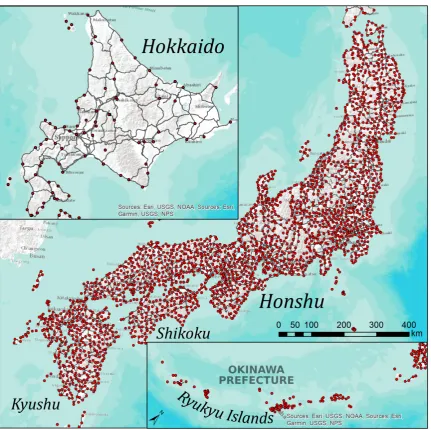
Figure 1. LAJ localities and the network of main roads in Japan. The mapping scale of the rather scattered Ryukyu Islands is smaller by a factor of 1.5.
Due to their potential isolating effect, coincidence of dialectal boundaries with political and natural 131
borders has often been tested, e.g. [61–63]. Derungs et al. [25] tested the impact of administrative and 132
cultural boundaries on dialect variance using spatial autoregressive models. In relation to Japonic 133
languages, Lee and Hasegawa [8] showed that ocean straits between Japan’s islands act as a barriers 134
that promote diversification. Nevertheless, effects of administrative boundaries within mainland Japan 135
have not been quantitatively tested for their isolation role in language. 136
Despite the fact that Japanese dialects are among the most thoroughly researched ones, the 137
explanatory power of geographic factors on linguistic variation has not been researched until lately 138
[14,15]. Japanese dialectology until recently, similarly to traditional dialectology in general, was 139
involved mostly in qualitative studies of characterising individual linguistic phenomena, e.g. [64–66], 140
and quantitative studies involving aggregation of multiple phenomena based on surveys, but excluding 141
geostatistical analyses. The latter line of research is exemplified in Tanaka’s work [67], tracking the 142
diffusion of Standard Japanese lexical features from the former and present capitals (Kyoto and Tokyo). 143
Since the end of the 19thcentury in Japan, the official language policy enforced using Standard Japanese, 144
dialectology and computational approaches have proven the split between Japanese and Ryukyuan, the variety of Okinawa prefecture in southern islands, often considered separate languages [14,75,76]. 155
Due to this, Okinawan varietes are outliers in the LAJ as well. Besides, the northernmost large island, 156
Hokkaido is, on the one hand, less densely populated than other parts of Japan and, on the other hand, 157
has less distinct dialects because of its more recent large-scale settlement (starting at the end of the 19th 158
century, mainly from Honshu), resulting in more mixed and standardised varieties. 159
The data used for this research stems from the digitised LAJ survey data (LAJDB) [74]. LAJ 160
was produced at the National Language Research Institute (NLRI), today called National Institute of 161
Japanese Language and Linguistics (NINJAL), presenting the recorded material of a large-scale survey 162
conducted between 1957 and 1965. Throughout Japan, 2400 localities were surveyed, interviewing one 163
male respondent, born between 1879 and 1903, at each locality. The survey locations are mapped in 164
Figure1, together with the most important regions of Japan, the main islands, showing the main roads. 165
1.3. Aims of the Research 166
In this study, we investigate the driving factors of dialectal variation and quantify contact between 167
communities at a historical scale making use of the potential of theories of GIScience and variationist 168
linguistics, and tools used in historical GIS. We identify the missing locality level dialectometric 169
analysis of Japanese dialect data as the main research gap and focus on providing a comprehensive 170
methodology to address it. 171
We establish a linguistic distance between localities based on the digitised LAJ data (termed 172
LAJDB). We perform an overlap analysis across the variants used throughout Japan, in search of spatial 173
clusters without taking space explicitly into account. Besides, using multidimensional scaling (MDS) 174
on the linguistic distance calculated, we provide a contrast to classic dialect maps often showing the 175
presence of dialect areas and by sharp borders, e.g. [77]. 176
Due to the fact that linguistic variables chosen for dialect surveys usually exhibit spatial variation, 177
we may assume that spatially autocorrelated geographic factors explain a considerable proportion of 178
the variation in our survey data as well. We are motivated to research the historical contact potential 179
by the assumption that preceding environmental settings impact language variety, in relation to the 180
concept of apparent time. Potential contact might depend on accessibility rather than just distance, 181
especially in case of an archipelago nation such as Japan, inviting the question of how to best estimate 182
contact in such a scenario. Because of the regional differences in Japan, as in the case of the Ryukyu 183
Islands and Hokkaido, we employ a local approach beside performing global calculations. 184
We build the following models: 185
• A series of models estimating contact potential: 186
– before the time of infrastructural development, using network of least cost paths based on 187
digital elevation models (DEM), 188
– at present, using today’s road network for calculating travel distances and travel times 189
– independent of time, using the great circle distances between localities. 190
• A model estimating the potential influence between communities based on their population 191
density and an inverse-distance association similar to the law of gravity . 192
• Finally, we test the separating effect of administrative boundaries, on the one hand the 193
6
deemed to have affected the language variation before the LAJ respondents’ age of mother 195
tongue acquisition, due to restriction of free movement [78], and on the other hand their modern 196
counterpart, theprefectures(Japanese:ken). 197
The methodologies presented in this work contribute to the characterisation of the the Japanese 198
lexical dialectal landscape. The methodology accounts for geographic factors in a differentiated way, 199
and revisits associations among linguistic variables and the spatial patterns of their variants through 200
quantitative analysis. Based on this, the conventional dialect area formation theories of Japanese (often 201
coercing dialectal boundaries onto natural and man-made boundaries, much like the perception of 202
laypeople would delimitcontinuousvariables) can be revisited. Further, the models worked out for this 203
study can be easily scaled to data in other languages or other data in digital humanities with similar 204
distribution and granularity. 205
2. Materials and Methodology 206
As this work conducts a comprehensive quantitative analysis of language data contrasting it to 207
several different spatial factors, the structure of the present section needs some explanation. First, we 208
introduce the LAJDB. Second, we present the data processing steps and the related overlap analysis. 209
Third, we detail the design of the linguistic distance measure. Fourth, we account for the spatial 210
association of linguistic distance by MDS. Fifth, we walk through the different analyses implementing 211
the distance based spatial models described in Section1.3. We will use the generic term ’spatial 212
distances’ for the measurements in these models which estimate contact potential based on spatial 213
factors. Finally, we present the methodology for testing the impact of administrative boundaries. 214
Similarly, in Section3the results of each analysis and their interpretation is presented sequentially, 215
followed by a comprehensive concluding section. 216
2.1. Dialect Data – Linguistic Atlas of Japan 217
This study uses digitised and publicly available data from the LAJDB [74]1. LAJ is a dialect atlas 218
based on a survey conducted from 1957 to 1965 by the National Language Research Institute (NLRI), 219
the predecessor of NINJAL. The atlas was published in six volumes between 1966 and 1974. The atlas 220
contains 285 questions (termedvariablesin this work), mostly aboutlexical variation(the linguistic 221
term for variation in vocabulary), including common nouns, verbs and adjectives. 2400 localities were 222
surveyed by 65 fieldworkers by means of personal interviews. At each location, one respondent (a 223
male in almost all cases) was interviewed. The respondents were born and grew up at the survey 224
location or lived there without interruption from the age of 3 to 15 [74]. Most respondents of the LAJ 225
can be described as"NORMs", i.e., non-mobile, old, rural males [79], which in dialectology translates 226
to the research aims of such surveys finding the"oldest"possible,"authentic"dialectal forms present, 227
sometimes called the"base dialect". Due to the sampling strategy of LAJ (one NORM per locality), the 228
variationwithinlocalities is hidden. However, in some localities, two or more linguistic forms of some 229
linguistic variables were recorded from the same respondent. The fact that approximately 80% of all 230
localities were agricultural communities [20] also shows that NLRI wished to record a variation as 231
little impacted by urbanisation and standardisation as possible. About six localities are surveyed every 232
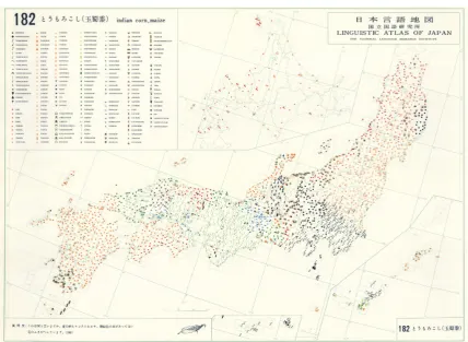
1000 km2, except for Hokkaido. Figure2shows LAJ map nr. 182, presenting the distribution of the 233
variants used to express’corn’or’maize’. 234
We used 37 variables from LAJDB, available online2at the time of the research. The majority of 235
these variables focuses on basic vocabulary in relation with body parts, weather and time, animals and 236
plants, and levels of kinship. We identify this focus as a risk factor for our results being representative 237
of the LAJ. 238
Figure 2.Example map from the LAJ (Nr. 182 -’indian corn, maize’).
According to the concept of apparent time, we infer the potential contact patterns that might have 239
shaped the dialectal landscape before and at the time of the respondents’ mother tongue acquitisition. 240
Apparent time constructs have been used to infer the synchronic manifestation of a language change 241
in progress for various levels of linguistics [80,81]. It is claimed, however, that rates of change vary 242
by linguistic level (e.g., lexicon, pronunciation, morphology, syntax), with lexicon, i.e. the function 243
of words, their semantics and meaning, having a higher rate of change compared to other linguistic 244
levels [82]. We identify this as a potential risk for our apparent time approach. 245
2.2. Categorisation of the Dialect Data – Overlap Analysis 246
We start the dialectometric analysis by discovering the associations across the dialectal variants in 247
the 37 variables. Doing so we aim to find out whether certain variants are used together, but without 248
the bias usually present in traditional analyses, i.e. the map comparison dialectal analysts usually do 249
in search of individual variables’ similar patterns. Lexical variation present in certain linguistic items 250
can be immense, and this is also recorded in LAJDB. To reduce variation, we categorise theanswer 251
variantsfor each variable based on the original LAJ maps3. In LAJ maps, variants’ symbols are grouped 252
together based on phonetic similarity, historical relations and semantic categories (see the map legend 253
example in Figure3). Using the groupings present on the maps, the number of answer categories is 254
reduced from approx. 10-500 to 3-15 per variable. We term the resulting categoriesvariant categories. 255
To measure the overlap of usage between two categories, we use a measure of association similar 256
to the Jaccard index, as we calculate the intersection over the union of the users of the variant categories. 257
For a pair of variant categories, we take the number of localities where the variant categories are 258
used concurrently (overlaps) and divide it by the number of localities where only one of the variant 259
8
Figure 3.The legend of the example LAJ map Nr. 182 in Figure2. The variant categories in our research were set up based on the groupings visible in such legends.
categories is used (divergences). A similar approach is present in previous research e.g. Uiboaed et al. 260
[83], who used the statistical ordination method correspondence analysis (CA) in dialectology, but for 261
finding associations across localities. 262
Based on the correspondence matrix of variant categories, Figure6shows a graph of associations 263
for each variant category with all others, independent of geography, created using theRpackage 264
qgraph[84]. 265
2.3. Linguistic Distance – Quantifying the Dialect Variation across Localities 266
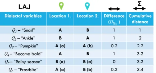
Based on the variant categories, we calculatelinguistic distancesfor each pair of survey localities. 267
Our linguistic distance measure is similar to theNC-measure of Kumagai [74] and theRIV-values 268
of Goebl [34]. For a locality pair, our measure is defined based on the sum of differences for each 269
of the 37 variables. In turn, the difference for each variable between localitiesiandjalso takes into 270
account differences within a variant category (see also Figure4). If for a linguistic variable all answers 271
in localitiesiandjare in different variant categories, then a linguistic distance of 1 is assigned to this 272
locality pair for this variable. Ifiandjhas answers in the same variant category, but not exactly the 273
same variant, the linguistic distance grows by a flat rate of 0.2. Finally, if the answer(s) iniandjfor this 274
variable completely overlap(s), the linguistic distance does not grow. The linguistic distance between 275
localitiesiandjis then summed: 276
Dlingij = ∑DQ
Figure 4.Calculation of the linguistic distance between two localities. Uppercase letters stand for the variant category while lowercase letters stand for the actual variantwithinthe variant category.
wherenis the number of variables with answers from both respondents (both localities),DQ ∈
277
{0, 0.2, 1}is the grade of divergence or correspondence for an individual variable, regarding localitiesi 278
andj. For a forged example, see Figure4. 279
For linguistic distance calculations missing answers are not taken into account. In case answers in 280
iandjare in the same variant category, the answers might be fairly similar to each other or wildly 281
different. Variant categories impose sharp boundaries in an otherwise fuzzy and diverse continuum 282
of lexical variation, often diverging based on the pronunciation of the linguistic item. Although for 283
pronunciation the Levenshtein distance is often used in dialectology for defining the distance between 284
two vectors, e.g. [32,33], we may not use this approach because of the variants that are categorised 285
together due to a sound of interest, however completely diverge, e.g.,’nanmai’and’banbarakibi’in 286
the example variable in Figure3). Two variants in the same variant category can also be a pair of 287
compound words with the two parts swapped. The histogram of variant occurrences in a variant 288
category, however, has a long tail, similar to a Zipf-curve [85] (p. 384). In most cases this means that 289
the majority of answers iniandjthat fall into a certain variant category are actually also the same 290
variant. We decided for a flat rate of 0.2 when noting linguistic distances within a variant category 291
because of such discrepancies within variant categories. We tested the effect of flat rates’ from 0.1 to 292
0.5 on the resulting linguistic distance and the correlation coefficient always stayed above 0.97. 293
Having created the linguistic distance matrix, the linguistic distances can be mapped from any of 294
the 2400 localities (example maps in Figure7). 295
2.4. Discovering the Spatial Association of Linguistic Distance by Multidimensional Scaling 296
Calculating the linguistic distance matrix allows the discovery of the encapsulated spatial 297
association. As we created a distance matrix based on the 37 variables, multidimensional scaling 298
(MDS) can be performed directly on this 2400*2400 distance matrix, containing thecontinuousvalues 299
for linguistic distance. Practically, MDS reduces the extent of a multidimensional point cloud into 300
a space as low-dimensional as possible (most research reports two or three, similarly to Principal 301
Component Analysis). “Each dimension extracted by multidimensional scaling represents a specific 302
pattern of regional variation and can thus be interpreted in isolation. However, it is more common to 303
display two or three dimensions simultaneously” [86] (p. 257). In our case, clusters of data points in a 304
three dimensional space can be interpreted as localities (actually respondents) similar to each other 305
with regards to the multitude of dimensions. Assigning the values along these dimensions to RGB 306
(Red, Green, Blue) colour values, the resulting colours can be used to find spatial associations when 307
the locations are mapped (Figure9). As a consequence, MDS supports the investigation of dialect 308
area formation, a central topic in linguistic geography. Moreover, dialect areas often defined by the 309
traditional methods of searching for ’isogloss bundles’ can be revisited based on a larger number of 310
10
2.5. Estimating the Dialect Contact Potential 312
In effect, our models in Section1.3test correlations of linguistic distance with the different ’spatial 313
distances’ (as estimations of contact potential) at the global level and in different functional subsets, 314
the main islands of Japan, using Pearson’s product-moment correlation. As logarithmic relationship 315
with geographic distances was commonly found in previous research [26,30,39], we perform tests with 316
the logarithm of the explanatory variables as well. Statistical significance of the differences between 317
the resulting correlation coefficients is tested by means of az-score suggested by Meng et al. [87], 318
implemented inRpackagecocor[88]. 319
2.5.1. Great Circle Distance 320
In order to account for the possibility of contact between communities, most dialectometric 321
research, by default, uses the linear or Euclidean distance. Therefore we also use the Euclidean distance 322
as a baseline for testing the explanation power of other distance based explanatory variables. We 323
obtained great circle distances (GCD), i.e., Euclidean distances on the surface of Earth, using the’fields’ 324
package [89] inR, for each locality pair. We perform correlation tests with the linguistic distances and 325
GCD, together with their logarithms. The distribution ofGCDhas a strong positive skew with the 326
largest distance being 2964 km between Western Okinawa and Northern Hokkaido. 327
2.5.2. Travel Distance 328
GCDmight overestimate the potential contact between communities, as contact paths are seldom 329
straight due to obstacles in the landscape, such as mountains, rivers or lack of roads. Using the ArcGIS 330
Data Collection Road Network in Japan (state of 2016) [90], we calculated shortest travel distances 331
(TD) for locality pairs in ArcGIS with the help ofarcpyscripts. The resultingTDmatrix has limitations, 332
however, as it only contains values for locality pairs that are reachable on land, with missing values 333
accounting for 29.27% of all locality pairs. This leaves little results for Okinawan islands and other 334
smaller islands not connected to the main islands Honshu, Kyushu, Shikoku and Hokkaido by bridges. 335
Shikoku and Kyushu are connected to Honshu by road bridges, but Hokkaido is not. The network 336
available did not include ferry routes, therefore giving unrealistic contact patterns in relation of locality 337
pairs on Kyushu, Shikoku and Honshu as well, practically moving the agents through bridges, even if 338
a ferry was available. 339
The distribution ofTDhas a positive skew with the largest distance being 1999 km within the 340
connected islands of Honshu, Shikoku and Kyushu. However, due to the presence of large distances 341
and with a large number of locality pairs taken into account, the difference betweenGCDandTDis 342
assumed to level out. Because of this we expect the difference in their explanatory power to be more 343
meaningful in the regional subsets. 344
2.5.3. Travel Times 345
Shortest paths in networks are, however, not always the fastest paths, as they do not take into 346
account the quality of the roads and the permitted speed. Therefore the time necessary to reach a 347
certain point is hypothesised to be a better estimation for potential contact between communities. 348
Gooskens [21,91] and Jeszenszky et al. [53] tested the correlation of travel times and Norwegian 349
and Swiss German dialect differences, respectively, and found that historical travel times explain 350
more variance in the linguistic distance than contemporary travel times. UsingOpen Source Routing 351
Machine(OSRM) through its implementation inR(package’osrm’) [92], we obtained present day travel 352
times (TT) by individual transportation. OSRM sends batched requests to theOpen Street Map(OSM) 353
routing client and gets back travel time values. As OSM navigation takes ferry routes into account, 354
the resultingTTmatrix has a missing value rate of only 3.14%. However, ferry connections towards 355
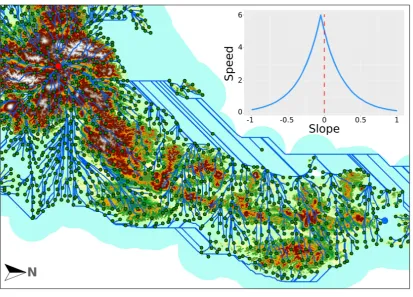
Figure 5.Representation of the least cost paths in our model with a starting point in the Japanese Alps (Nagano prefecture). Tobler’s hiking function is shown in the top right corner with speed (km/h) as the function of slopes (proportion).
transport faster than car transport, such as airplanes and theshinkansenhigh-speed railway lines of 357
Japan,TTobtained might underestimate the present day contact potential between localities. 358
Nevertheless, thisTTmatrix represents contact paths some 50 years after the dialect survey and 359
more than a 100 years after the time of the respondents’ mother tongue acquisition. We might assume, 360
however, that with the increasing speeds in the system, the proportions in travel times have not 361
significantly changed during these times, disregarding high-speed connections, which our OSM-based 362
model also lacks. The distribution ofTThas a strong positive skew with 94% of the values under 36 363
hours. 364
2.5.4. Least Cost Paths and Hiking Times 365
As it is commonly assumed that historical contact patterns would explain today’s dialectal 366
landscape more, we aimed to model the potential contact paths in Japan before the infrastructural 367
boom brought by the industrial revolution. In Japan the industrial revolution began in the 1870’s, not 368
much before the LAJ respondents’ mother tongue acquisition. Therefore we assume the effects of ’intact’ 369
relief and environment to have had a substantial effect on the dialects surveyed. Our assumption is 370
that least cost paths, the most natural paths of contact between communities, were predominantly 371
unchanged for centuries before the industrial revolution and over land they would substantially 372
depend on relief. We also assume that the first paved roads and other measures for speeding up 373
transportation (earliest railways) were implemented along least cost paths. Our model is based on the 374
10 m resolution digital elevation models (DEM) in the Fundamental Geospatial Data provided by the 375
Geospatial Information Authority of Japan [93], which we resampled at 100 m resolution. 376
Using Tobler’s hiking function [94] (Eqn. 2), which defines average walking speed as the function 377
12
pairs, similarly to [25,95]. With its peak walking speed for slight downward slopes, the function 379
is asymmetrical, marked with a shift of 0.05 in the exponent (the shape of the function is shown in 380
Figure5): 381
V=6∗e−3.5∗|S+0.05| (2)
whereVis the velocity of walking andSis the slope value in radians. 382
This asymmetry means that in most cases the resulting least cost paths and subsequently the 383
hiking times differ depending on the direction of the path calculated between localities. As contact 384
between any communities is bidirectional, for each locality pair we take the mean of the resulting 385
hiking times along the least cost path . 386
In order to calculate least cost paths between localities separated by sea (i.e., where a path over 387
a DEM is not available), we allowed "seafaring". The speed of seafaring has been defined as 2.5 388
times larger than land movement on flat surface, to match the premise of pre-infrastuctural contact 389
paths on land with that of sailing median speeds before steamboats. The speed was established 390
based on Casson’s calculations [96], who gathered travel speeds of the Mediterranean in the antiquity. 391
This relatively slow speed is an average, taking into account favourable and unfavourable wind 392
conditions. This slow speed also balances to a degree the fact that the agents in the model start 393
sailing at the exact time they reach a port, which would be unimaginable in reality. To restrict the 394
movement as much as possible to plausible shipping routes we restricted "sea entry" to ports that were 395
important in the Edo-era (1603-1868), based on data from Saito’s research [97]. To be able to reach all 396
localities, including those on smaller islands, further "ports" were added to the model. We allowed 397
only near-shore seafaring, limiting the model’s inclusion of sea to 50 km off the coast. Besides, we used 398
the natural state of Japan’s coastline, before the land reclamations around port cities took place mainly 399
after WWII. ArcGIS 10.6 andarcpywere used for the model calculations. The crucial location of ports 400
from the point of view of potential contact is visible on Figure5. Because of some obvious limitations 401
of the model, such as the lack of land cover, the 100 m resolution and not taking fatigue or constant 402
availability of ships into account, results from our model should be taken with a grain of salt. 403
As we allow for sailing beside moving in the DEM, there are no points pairs in our model that are 404
not connected. In the remainder of this paper, we will term the measurement resulting from this model 405
hiking time(HT). Of all our explanatory variables, the distribution ofHThas the weakest positive skew, 406
with a median inHTaround 90 hours and maximum of 384 hours. 407
2.5.5. Linguistic ’Gravity’ Index 408
To estimate the probability for actual contact across localities beyond accessibility, we calculated a 409
gravity-like index, estimating the potential’interaction’between communities to which survey locations 410
belong, based on their geographic distance and their population densities. It is expected that more 411
populous communities would interact more with each other, even if they lie farther away. Besides, 412
such ’gravitational’ model is assumed to align with commuting and other communication patterns 413
between smaller and larger settlements, i.e., villages would have more interaction with a nearby city 414
than with the surrounding villages. The original of this model was worked out by Trudgill [11], and 415
the resulting index is often called Trudgill’s linguistic gravity index (TLGI). In Szmrecsanyi’s words 416
the inverse-square law of gravitation "postulates that the interaction between two dialects decreases 417
with increasing geographic distance but this effect is counterbalanced by larger speaker communities" 418
[52] (p. 222). Based on the Newton’s law of gravity,TLGIis formulated as Eqn. 3.: 419
Mij=
Pi∗Pj
Dij2 (3)
whereMis the index of potential interaction (TLGI),Pare the populations of the two localities in 420
of the 1 km grid census grid, for privacy reasons. Thus for each locality, the same amount of grid cells are considered. This way thePweights in our model actually correspond to a neighbourhood 431
level population density. On the downside, the distribution of population assigned to our localities 432
does not reflect the actual population present in the municipalities, especially regarding metropolises. 433
Although the actual population would be in the millions in several municipalities and in the 100’000s 434
in dozens of municipalities, ourPweights never go over a million and they are over 100’000 in the top 435
one hundred localities, most of which pertain to areas of metropolises. This is thought to skew the 436
gravitational force metropolises exert over long distance. However, the locally stronger gravity (due 437
to several localities falling into today’s metropolitan areas) might better reflect the communication 438
patterns characteristic of the Meiji-era. 439
AsGCDwas available for all locality pairs, we used it as the distance measure inTLGI. 440
A logarithmic correspondence is expected between the linguistic distance andTrudgill’s linguistic 441
gravity index (TLGI). 442
The gravity index is extremely skewed to the right with most localities incapable of direct contact 443
(withTLGIvalue converging to 0) and nearby populous localities having a very strong impact on 444
each other. The latter are basically the survey locations in metropolitan areas where the respondents 445
practically belong to the same city rather than their 2.5 km neighbourhood, and thus their dialects 446
should theoretically be the same. While the largest index values are in the thousands, 99% of the values 447
stay under 0.2. 448
2.6. Explaining Linguistic Variation through Administrative Boundaries 449
We tested the separating effect of administrative boundaries of domains and prefectures, described 450
in Section1.3. These boundaries restricting the movement of their inhabitants is claimed to be one of 451
the key factors in the formation of the latest Japanese dialects [78]. We test the effect of boundaries of 452
68 domains at the time of their abolition in 1868 on the lexical variation, together with the effect of 453
prefectures. However, the boundaries of the 47 prefectures follow domain boundaries very closely 454
and are virtually unchanged since 1888. It can be assumed that those domain boundaries were kept as 455
prefecture boundaries that denoted an important isolation factor anyway. 456
The effect of administrative boundaries was analysed using the non-parametric Mann-WhitneyU 457
test (also known as the two-sample Wilcoxon rank-sum test). The null hypothesis is that both samples 458
are from the same population and theUtest determines whether two independent samples were 459
selected from populations having the same distribution. Unlike thet-test, theUtest does not require 460
the assumption of normal distributions and unlikep-values, theUtest is not affected by sample size. 461
We perform a subsequent Vargha-Delaney effect size test [98] on domain and prefecture boundaries, 462
and report the probability that a value from one group will be greater than a value from the other 463
group, that is, we show the stochastic dominance of one group, when present, unaffected by sample 464
size [99]. The groups used in the tests are the following: 465
1. Both localities are located in the same domain or prefecture (termed’within’group) and 466
2. The localities are separated by prefectural boundaries (termed’separated’group). 467
This grouping fulfills the requirement of the U test, assuming that the observations are 468
14
are different and the linked Vargha-Delaney A value shows the direction and probability of the 470
difference. 471
The tests are done for each domain and prefecture separately and also as an aggregate. In order 472
to compare the effects of domains and prefectures, we performed the tests for prefecture boundaries 473
in the area covered by domains in 1868 (practically excluding Hokkaido and Okinawa, which were 474
incorporated later into Japanese administration). Due to their more historical role, we assumed the 475
domain boundaries to have a larger effect on the variation, resulting in larger linguistic distances for 476
the group’separated’by boundaries. 477
As Japan’s area is large, its administrative regions vary in size greatly, and internal migrations 478
assumed lower in volume before and at time of the of the LAJ respondents’ mother tongue acquisition 479
than today, we performed the above tests with various distance cut-off measures. That is, we restricted 480
the locality pairs considered in the tests to various distances, between 50 km and 200 km. This assumes 481
that effects of isolation inflicted by the boundaries would manifest themselves with a relatively small 482
distance cut-off already. 483
3. Results and Interpretation 484
3.1. Association Across Linguistic Variants Disregarding Space 485
The association graph in Figure 6visualises the variant categories that are used together in 486
the survey locations and the strength of the connection, proportional to the Jaccard index. Parallel 487
to analyses in traditional dialectology delimiting dialect areas based on isogloss bundles, e.g. [36– 488
38], this overlap analysis shows the degree to which dialect areas can be discovered based on the 489
37 lexical variables considered, but, importantly, independent of geography. Having no spatial 490
association thus means that our overlap analysis avoids the spatial bias that is present when creating 491
isoglosses by drawing lines on maps. The strongest connections ultimately mean exclusive overlap 492
of the areas covered by the variants in question. The network visualisation in Figure6uses the 493
Fruchterman-Reingold algorithm, which also conveys that the positions or distances of nodes are 494
not supposed to be spatially interpreted [84,100]. The color saturation and the width of the edges 495
corresponds to the absolute weight and scale relative to the strongest weights in the graph. 496
In Figure6, two main clusters can be identified, with the association strength gradually fading 497
out around their centres. The larger cluster is associated with the Standard Japanese variants, usually 498
found spread across large areas in the main island Honshu. The more central the node’s position within 499
such cluster, the more the variant category overlaps with others, signaling their ubiquitous distribution. 500
The spatial relations of such variant categories can be verified on LAJ’s individual variable maps. The 501
smaller cluster on the right is associated with variant categories used in Okinawa, hinting at the fact 502
that variants used here usually do not overlap with the variants used in Honshu, Shikoku or Kyushu. 503
The close-knit cluster lets the observer associate on a high grade of exclusivity, except for its top right 504
part, which represents variant categories used on the Sachishima-islands, the westernmost island 505
group in the Ryukyu Islands, with what appears to be a distinct dialect based on our data. 506
Based on the 37 variables however, the classic of dialect areas’ definition established using isogloss 507
bundles cannot be proved or disproved. On the one hand, even the close-knit clusters of overlapping 508
variant categories include only a few of the variant categories rather than one variant category from 509
most variables. On the other hand, the variant categories in the largest cluster are used throughout vast 510
areas in Honshu, a finding which would not qualify to building dialect areas. This pattern invites the 511
question whether the linguistically opposing concept, the dialect continuum theory can be warranted 512
based on the data available. This interpretation is in connection with analysing the results from the 513
Figure 6.Graph presenting the occurrence overlap in variant categories, based on the Jaccard-index. Survey questions represented by the same colour are not related. For exampleQ188_5means the 5th variant category in survey question nr. 188 in the original LAJ.
3.2. Linguistic Distances Mapped 515
Calculating the linguistic distance matrix allows to produce maps with different reference 516
locations, i.e., presenting linguistic distances in reference to certain localities. This kind of visualisation 517
goes back to Goebl’s dialectometry [34,101]. Figure7maps the linguistic distance from the following 518
six localities: the north of Hokkaido, a rural site in Aomori prefecture in the north of Honshu, Tokyo, 519
Kyoto, Matsue city in Shimane prefecture in the west of Honshu, and Okinawa’s capital city, Naha. 520
Tokyo (formerlyEdo) and Kyoto are the present and the past capitals and cultural centres of Japan, and 521
therefore thought to have affected the language of the whole country by being the starting points of the 522
(hierarchical) diffusion for many linguistic innovations [73,102,103]. Aomori in the northern extremes 523
of Honshu is far away from both capitals, and as such, it is associated with preserving dialectal features 524
less affected by standardisation. Matsue is the centre of the so called Umpaku dialect area which 525
has a unique historical aspect. Hokkaido has been settled by Japanese primarily from the end of 526
the 19thcentury, exactly when the respondents were acquiring their mother tongue, from different 527
parts of Japan but mostly the Tohoku (NW) and Hokuriku (the western shore of central) areas in 528
Honshu. Because of this, the language history is not deep and respondents are assumed to inherit their 529
ancestor’s language leading to a dialectally mixed area with Standard Japanese having gained ground 530
more easily. It is not attested in our 37 variables whether the antecedent Ainu population of Hokkaido 531
affects the variants used. Lastly, Okinawa as an archipelago used to be a semi-independent kingdom 532
mostly isolated from imperial Japan until incorporated as a prefecture in 1879, also shortly before the 533
LAJ respondents’ mother tongue acquisition. Because of the historical isolation, vast differences are 534
expected between Okinawan and "mainland" varieties. 535
In general, Figure7shows that the closer a locality is to the reference locality, the smaller their 536
linguistic distance, but Okinawa tends to show uniformly larger linguistic distances, while Hokkaido’s 537
localities are never extremely different from the reference localities. The northerly Hokkaido locality 538
seems to be lexically close to various areas, attesting a mixture of dialects or the degree to which 539
Standard Japanese is used in different parts of the country. Interestingly, the north of Honshu (Aomori, 540
Tohoku) are some of the linguistically most different areas from this locality. The Aomori locality 541
16
Figure 7. Linguistic distances map with six reference sites from top left to bottom right: Northern Hokkaido, rural location in Aomori prefecture, Tokyo, Kyoto, Matsue city (Shimane prefecture) and Naha, capital of Okinawa prefecture.
being different. At the same time the southern tip of Hokkaido seems more similar, which hints on 543
the language connection present throughout history. Linguistic distances to Tokyo (the birthplace of 544
Standard Japanese) tend to be smaller throughout Honshu, and most Hokkaido localities express a 545
similarity with it. The largest distances are found in the north of Honshu (Tohoku) and the south 546
of Kyushu, the geographically farthest areas. Kyoto, as the former capital is expressly similar to 547
its surroundings, in the so called Kinki area, with its similarity gradually fading away by distance 548
and levelling to the highest differences in the north of Honshu and south of Kyushu. Interestingly, 549
similarity between the Tokyo and Kyoto area is not salient in these maps, based on our set of variables. 550
The area looking similar to Matsue spreads farther away than Kyoto’s and also looks concentrical, 551
with the exception of Hokkaido. Okinawa is, finally, uniformly different in all maps with reference 552
points in the larger islands. Its own reference map centred in Naha, the capital city of Okinawa shows 553
extreme difference with all other provinces of Japan and even in the Okinawa prefecture itself, the 554
Sachishima-islands in the west present a relatively large difference. 555
Based on the linguistic distance matrix, for each locality an average linguistic distance can be 556
calculated to all other localities by taking the mean of each matrix row. Mapping these average values, 557
used also in [53], adds a technique to Nerbonne’s inventory of mapping aggregate variation [28]. The 558
resulting map in Figure8can thus be interpreted as a degree of overlap between the locally used 559
lexicon and all other localities’ lexicon. Importantly, similar colours do not correspond to linguistic 560
similarity, but to mean difference from all localities being similar. Although the lexical distance is 561
calculated based on only 37 variables, the map shows several interesting points. The most conspicuous 562
interpretation of the map is that Okinawan varieties are the most different from all others on average, 563
as expected. The localities closest to all other sites are found on Hokkaido, attesting the mixed nature 564
of the local varieties. In Honshu the area spanning from North of Kanto (the area containing Tokyo) to 565
the West of Kansai (the area encompassing Kyoto, Osaka, and the cultural centre of Japan before the 566
Edo-era) is a seemingly average area, fading out into the extremes of the three main islands: to the 567
Figure 8.Average linguistic distance map. Colours of each point correspond to the survey location’s average linguistic distance toward all other survey location.
3.3. Dialectal Variation in Space 569
Having performed the multidimensional scaling (MDS) on the 2400*2400 linguistic distance 570
matrix, we can represent the dialectal variation in a three dimensional space, which is readily 571
interpretable. These three dimensions are assigned to the RGB colours. Interpreting the similarly 572
coloured clusters and spatial areas similar in either the 3D plot or the map in Figure9is practically 573
equivalent to finding similar survey sites with regards to all 37 variables and therefore to accounting 574
for dialect areas. Figure9excludes the Ryukyu Islands (containing Okinawa) due to their large 575
linguistic distance from all other parts of Japan. Despite the removal of the outlying Ryukyu Islands, 576
no genuinely isolated clusters are visible in the 3D plot. Although contrasting colours and certain 577
central areas can be identified in the map, such as the northern part of Honshu, the Kanto area centred 578
around Tokyo, or the south of Kyushu, the transitions in between remain gradual, attesting for the 579
theory of dialect continua. As expected, Hokkaido’s localities seem to be mixed and brownish in 580
colour, which indicates equal mixture of RGB colours and thus centrality. In essence, there is a contrast 581
between the MDS map based on the 37 variables at hand, and the classic area formation map of 582
Japan, e.g. [77]. The boundaries of dialect areas usually bordered by sharp lines can be considered 583
as a representation of some core varieties based on the MDS map, painting a fuzzier picture of the 584
18
Figure 9.Multidimensional scaling map excluding Okinawa. The more similar colours are, the smaller the linguistic distance. The inset 3D plot shows the clustered relationship of the localities with regards to the three main dimensions.
An additional MDS conducted only on the Ryukyu Islands revealed that isolated clusters can 586
be found based on the 37 variables, despite the small subset. Having found four isolated clusters – 587
namely, from West to East, the Yaeyama Islands, the Miyako Islands, the Okinawa Islands (containing 588
the capital), and the Amami Islands (belonging to the Satsuma domain of South Japan since 1624, 589
rather than the then Ryukyu Kingdom) – hints on the historical isolation not only between the Ryukyu 590
Islands from mainland Japan, but also within itself. 591
3.4. Correlations with Spatial Measurements 592
We calculated several values estimating the potential of dialect contact across localities in the LAJ. 593
For the continuous values, we built spatial distance matrices similarly to the linguistic distance and for 594
all matrix pairs, Pearson product-moment correlation was calculated. Figure10shows the correlation 595
coefficients across the explanatory variables for the entire survey area. A high correlation present 596
amongGCD,TD,TTandHTis not surprising, given the size of Japan. These values are negatively 597
correlated with the logarithms of theTLGIvalues, as they represent aninfluence, therefore similarity, 598
Figure 10.Correlation crossplot of the distance based explanatory variables.
It is expected that the logarithm of the spatial distances will have a greater explanatory power 600
on the linguistic variation due to the following. While linguistic distance can grow up to a certain 601
degree only (i.e., until total dissimilarity), spatial distance can constantly grow. It is expected (similarly 602
to most dialectological studies) that in a large area, such as Japan, large linguistic differences will be 603
reached before the most extreme spatial distance from a certain point is reached. 604
Correlation coefficients with the linguistic distance for the entire survey area and the functional 605
subsets are given in Table1. We first compare the effects of the spatial distances (roows) and then 606
discuss the different data subsets (coloumns). As seen in Figure10, the correlation ofGCD,TD,TTand 607
HTare almost total so, unsurprisingly, all of them explain a similar amount of variance in the dialectal 608
differences. It is also due to this fact that we tested the travel distance (lengthwise shortest paths with 609
regards to the network) and travel time matrices coming from different resources rather than sourcing 610
both from OSRM. 611
The correlation ofGCDwith the linguistic distance is presented in a heatmap (Figure11), due 612
to the large number of locality pairs. Hexagons are coloured by the number of points (locality pairs) 613
in each cell, thus plotting the density of points. The correlation is undoubtedly positive, but solely 614
based on the plot, its linear or logarithmic nature cannot be warranted. The correlation tests reveal 615
that the logarithm ofGCDexplains slightly more variance in the linguistic distance (r=0.6462 andr 616
=0.6714, respectively). The difference, however, proves to be statistically significant based on Meng 617
et al.’sz-score [87] calculated using theRpackagecocor[88]. This test is applied for finding whether 618
any correlation coefficient is significantly different from another, given their difference and the sample 619
sizes. 620
The high correlation withTDshould be taken with a little skepticism due to the high rate of 621
missing values. The logarithmic correlation is significantly higher in this case too. With a much smaller 622
rate of missing values, the correlation obtained with contemporaryTTis lower than that ofGCD, 623
but its logarithm seems to match the logarithm ofGCD. The large number of locality pairs however, 624
renders this difference statistically significant. 625
Correlation values forHTand their logarithms are similar, but lower than the previously discussed 626
values, inviting the question whether our model is less valid for the estimation of dialect contact 627
(resulting in the dialect landscape of the first half of the 20thcentury) or whether dialect variation is 628
not governed as much by potential least cost paths as we determined at the scale of the entire country, 629
20
Figure 11.Linguistic distance plotted against the great circle distance in the entire survey area. The colour of each hexagon represents the number of location pairs’ value falling into it. Regression lines are plotted for showing the linear (in red) and the logarithmic (green) relation.
To level out the uncertainty due to missing values inTD, correlation with linguistic distance is 631
calculated for the subset of locality pairs where all spatial distance values are available (L¬N A). For
632
this subset, containing 70.7% of all locality pairs, the correlation coefficients are given in the second 633
row of Table1. These results, however biased by not taking into account distances between Okinawa, 634
Hokkaido and the three most populous islands, show that the spatial distance based estimations 635
of contact deliver very similar explained variance. We assume that this is due to the fact that the 636
overwhelming majority of locality pairs lack the possibility for direct contact because of large distances. 637
In such cases only indirect contact is present and thus the way we measure theinabilityof contact 638
makes little difference. This convergence at the global level invites the investigation of the local impact 639
of different estimations of contact. 640
Table 1.Correlation coefficients expressed as Pearson’sr. For each set the number of localities included are given in parentheses.L¬N Ameans the survey location pairs with no missing values, i.e. where all spatial distancescan be calculated. HSK stands from the set composed of Honshu, Shikoku and Kyushu. *Travel distance has a missing value proportion of 29.27% while **Travel times have a missing value proportion of 3.14%,$Okinawan location pairs have very few non-missing values forTDandTT.
Entire area (2400)
L¬N A ≈ 70.7%
Hokkaido (83)
Honshu (1666)
HSK (2125)
Shikoku (141)
Kyushu (318)
Okinawa (82)
GCD 0.6462 0.6672 0.2487 0.6488 0.6673 0.7391 0.7237 0.6999
log(GCD) 0.6714 0.7048 0.2339 0.6876 0.7037 0.7824 0.7544 0.7718
TD* 0.6613 0.6613 0.2564 0.6713 0.6606 0.7602 0.7246 0.3902$
log(TD)* 0.7058 0.7057 0.2441 0.7126 0.7055 0.7943 0.7561 0.4139$
TT** 0.5322 0.6681 0.1773 0.5023 0.6675 0.5456 0.5493 0.7573$
log(TT)** 0.6717 0.7087 0.2782 0.6622 0.7072 0.6923 0.7357 0.7454$
HT 0.5836 0.6718 0.2177 0.6605 0.6719 0.7548 0.6786 0.5739
log(HT) 0.6078 0.6834 0.2115 0.669 0.6845 0.7693 0.664 0.6848
TLGI1975 -0.5078 -0.5188 -0.3539 -0.4919 -0.5182 -0.6454 -0.5498 -0.6078
TLGI2005 -0.4695 -0.4862 -0.3407 -0.4627 -0.4855 -0.606 -0.4966 -0.584
WithinHokkaidolower correlation is expected, since the island has been populated by Japanese 641
forTLGI2005, -0.3407, is not significantly higher than for the logarithm ofTT, 0.2782, due to a low
number of samples. This means that contact patterns based on migration and hierarchy do not 652
characteristise dialectal variation in Hokkaido more than elsewhere. 653
Honshu is encompassing two thirds of the survey locations and most pairwise values for 654
explanatory variables could be calculated. The large distances within Honshu encompass mostly 655
indirect contact, rendering the spatial distance values to explain a similar amount of variance, with 656
TThaving the lowest values. However, due to the high number of samples most of these correlation 657
coefficients are significantly different, resulting in the logarithm ofTDbeing the best explanatory 658
variable. 659
Unsurprisingly, the resulting correlation coefficients for the united subset ofHonshu, Kyushu 660
and Shikokuresemble those inL¬N A. The nuanced differences present stem from incorporating
661
location pairs inL¬N Athat arewithinHokkaido or other islands with multiple survey localities. This
662
also demonstrates the degree to which the three most populous islands outweigh all other areas when 663
accounting for correlations at theglobalscale, inviting the question of testing correlations at (more) 664
local scales. 665
Shikokuhas the highest correlation coefficients of all subsets, with the logarithm ofTDscoring 666
the highest (0.7943), however this value is not statistically significantly higher than that ofTD,HT 667
and their logarithms, and the logarithm ofGCD, due to the small number of localities on Shikoku. 668
Theservalues mean that the spatial distance measures explain about 62% of the variance in linguistic 669
distances, leaving a much smaller room for other, sociodemographic variables to influence the lexical 670
variation. Because of this, it would be interesting to investigate the role of geographic factors in 671
linguistic variation on the island of Shikoku more in depth. Shikoku’s geography is defined by rugged 672
mountains, crucially defining the communication of the four prefectures located on it. The centres of 673
these prefectures are relatively isolated from each other, having partly better chances at communication 674
with Honshu via sea, e.g. [104]. 675
Kyushu’scorrelation coefficients are almost as high as Shikoku’s, with statistically no difference 676
betweenGCD,TD, their logarithms and the logarithm ofTT. The relatively lower correlation withHT 677
could be influenced by the fact that the number of Edo-era ports for the Kyushu subset is also relatively 678
low. This shows the propagating effect of small differences in local models and the importance of 679
limitations regarding the realistic estimation of contact potential. 680
In the case ofOkinawa, as an archipelago, the fact of not having roads in between islands renders 681
theHTas the potential interaction estimation similar toGCD, with the difference of elevated importance 682
of port access.TDand times data are retained for less than half of the point pairs. Correlation with 683
TLGIis relatively high for Okinawa, probably due to its relatively small size and the frequency of 684
access across islands might historically correlate with their population, which might not have changed 685
much in terms of proportions. However,TLGI1975is not significantly lower than the logarithm ofHT.
686
Huisman [14] notes that in the island languages "diversity is a reflection of time since divergence, as 687
a result of limited contact due to the geographic isolation of islands". High correlation of Okinawan 688
linguistic difference with the remaining explanatory variables means that even though Okinawa is 689
relatively small and its variation is very different from all others in general, linguistic differences 690
within Okinawa itself are large and spatially autocorrelated. Further, a large part of this linguistic 691
22
In each set of locationsTLGI has a lower explanatory power, which would mean that even 693
bigger cities are impeded from communication by long distances. It might, however, show that 694
the communication patterns across the country characteristic of the Meiji-era cannot be very well 695
explained by influence characteristics representing 1975 and 2005, despite them being scaled down to 696
local population densities. 697
3.5. Effects of Administrative Boundaries 698
We report the tests investigating the dialect separation effect of administrative boundaries in two 699
ways. On the one hand, Table2shows the aggregate effect of the boundaries, testing thewithinand 700
separatedgroups’ overlap when cumulated for all administrative regions. All Mann-WhitneyUtests 701
result in statistically significant separation values, therefore only their effect sizes are reported, by 702
giving the Vargha-DelaneyAand their interpretation as defined in theRpackageeffsize[105]. On the 703
other hand, Figures12and13map the underlying effect sizes contributed by each of the administrative 704
regions, prefectures and domains respectively, showing the results of the calculations with a 150 km 705
cut-off. The colours of the regions correspond to the effect size categories. Besides, density plots show 706
the distribution of linguistic distances in thewithinandseparatedgroups, respectively, withwithin 707
groups expected to have smaller values. 708
Vargha and Delaney’sAreports the probability that a randomly chosen value from one group 709
will be greater than a randomly chosen value from the other group. A value of 0.5 would indicate 710
stochastic equality of the two groups. A value of 1 would indicate that thewithingroup shows complete 711
stochastic domination over theseparatedgroup, and a value of 0 would indicate the other way around, 712
theseparatedgroup showing larger linguistic distances in all cases. 713
Table 2.Global results of testing the effect of administrative boundaries. The density plots for 150 km distance cut-off cases are presented in Figures12and13.
Boundary type Distance cut-off(km)
Vargha-Delaney A
Interpreted effect size
Prefectures(47) 200 0.2607 large
Prefectures(47) 150 0.3045 medium
Prefectures(47) 100 0.3473 small
Prefectures(47) 50 0.3793 small
Domains(68) 200 0.5387 negligible
Domains(68) 150 0.3513 small
Domains(68) 100 0.3725 small
Domains(68) 50 0.4079 small
In all cases, at the aggregate scale in Table2, locality pairs separated by the domains’ boundaries 714
show little to negligible stochastic dominance with regards to linguistic distance, which means that 715
having a domain boundary between two survey locations would not mean much bigger chances for a 716
higher linguistic distance. The small stochastic difference between thewithin domainand theseparated 717
groups is also visible in the density plot in Figure13. In contrast, for prefecture boundaries the higher 718
distance cut-off value we chose, the larger the effect size, reaching the medium and large categories. 719
In Figures12and13it is often the larger regions for which a smaller effect is present. However, 720
not all large prefectures show this pattern and actually some of the largest ones’ boundaries show a 721
large effect. In case of the domains, the three largest ones in the north of Honshu show smaller effects 722
while the other domains showing small and medium effect overlap the areas of the prefectures that 723
also show small and medium effect. Smaller effects of larger regions’ boundaries might be due to larger 724
possible linguistic distances possiblewithinlarge regions, which might go hand in hand with smaller 725
distances across its boundaries. But as it is not always the case, it is safe to say that spatial variation is 726
present. This spatial variation is also marked by boundaries that changed as domains were reorganised 727