Journal of Fluid Mechanics
http://journals.cambridge.org/FLMAdditional services for
Journal of Fluid Mechanics:
Email alerts: Click here
Subscriptions: Click here
Commercial reprints: Click here
Terms of use : Click here
Topographic Rossby waves above a random array of
seamountains
Kalvis M. Jansons and E. R. Johnson
Journal of Fluid Mechanics / Volume 191 / June 1988, pp 373 388 DOI: 10.1017/S0022112088001612, Published online: 21 April 2006
Link to this article: http://journals.cambridge.org/abstract_S0022112088001612
How to cite this article:
Kalvis M. Jansons and E. R. Johnson (1988). Topographic Rossby waves above a random array of seamountains. Journal of Fluid Mechanics, 191, pp 373388 doi:10.1017/S0022112088001612
Request Permissions : Click here
J . Fluid Mech. (1988), vol. 191, p p . 373-388 Printed in Great Britain
373
Topographic Rossby waves above a random array
of seamountains
By KALVIS M. JANSONS
A N DE. R.
JOHNSON
Department of Mathematics, University College London, Gower Street, London WClE 6BT. UK
(Received 17 December 1986)
The barotropic potential vorticity equation or topographic wave equation is not linear in topography: the solution structure for topography formed from a sum of obstacles is not the sum of solutions for the obstacles in isolation, even when these individual solutions have identical frequencies. This paper considers the mechanism by which normal modes of oscillation above one mountain are modified by interactions with its neighbours. Exact explicit solutions for the normal modes above
a pair of circular seamountains show that the interactions between the mountains rapidly approaches the large-separation approximation obtained by considering solely the first reflection of the disturbance of one mountain a t the other. For mountains of one diameter separation a t the closest point, the approximation is accurate to within 1
YO.
Perhaps surprisingly, coupling between two identical mountains is weak and resonance occurs between mountains and dales of equal and opposite height.The accurate approximate solutions enable consideration of the effects on a
mountain of an infinite set of randomly distributed neighbours. The ensemble- averaged frequency for a mountain of given height is determined in terms of the area fraction of the other mountains. The idea of an effective topography is introduced for the ensemble-averaged stream function : it is that (non-random) topography generating a stream function identical to the ensemble-averaged stream function. This differs markedly from the ensemble-averaged topography. The explicit form of the effective topography is derived for a set of right circular cylinders.
1. Introduction
The early experiments of Taylor (1923) show the large effects that even small obstacles can cause in rapidly rotating flows. Later experiments and analysis, as those of Gill et al. (1986), demonstrate that the whole evolution of oceanographic flows can be affected by small changes in bathymetry (i.e. bottom topography). Topographic or planetary vorticity effects appear to be important in large-scale flows over anything but the flattest of ocean floors.
374 K . M . Jansons and E . R. Johnson
as a superposition of the normal modes of the linear equation -the topographic Rossby waves of Rhines (1969). An isolated seamountain is, however, a poor model for regions of complex bathymetry. The present paper models such regions by a random array of mountains and dales, obtaining approximations of the normal modes of the system and assessing the effect of the presence of other mountains on the modes of a given mountain. As in the case of an isolated mountain, these normal modes determine the evolution of the linear system. This evolution should closely approximate numerical integrations (e.g. those of Bretherton & Haidvogel 1976) of the full nonlinear equation over strong (i.e. S much greater than unity) random topography.
In the following sections we determine the normal modes of a single mountain in an infinite random array of non-overlapping, finite mountains of area fraction c much less than unity (i.e. the change in the single-mountain mode due to the presence of the other mountains). We do not consider bulk oscillations of the whole system, as this topic is to be discussed elsewhere. For this bathymetry all contour lines are closed curves. Solutions with this constraint relaxed are discussed elsewhere.
Results from classical wave-scattering theory are not useful in this limit. Topographic waves cannot exist over a flat ocean floor, unlike electromagnetic and acoustic waves, which can travel in an unperturbed medium and are scattered by inhomogeneities. One way of avoiding this problem is to consider small random perturbations to existing topography (Thomson 1975) ; such techniques have been reviewed by LeBlond & Mysak (1978). However, in this study we consider a limit where the random perturbations are order-one occasionally, so retaining the nonlinear dependence on topography.
Section 2 considers briefly the well-known solution for a single mountain on an infinite plain, introducing the notation used in the many-mountain problems. Section 3 presents an approximate solution to the two-mountain problem, showing that the strongest resonance occurs between a mountain and dale of equal and opposite heights. The field seen by one mountain due to a second appears to rotate in the opposite direction to the natural mode of the first and thus lies far from resonance. The exact solution for the two-mountain problem, given in Appendix A, shows the approximate solution to be accurate to within 0.5% for mountains separated by more than one radius. Section 4 gives the results for an infinite random array of mountains, introducing the idea of an effective topography to describe the structure of the ensemble-averaged stream function in the neighbourhood of a given mountain. The results are discussed in $ 5 .
The linear barotropic potential vorticity equation for small fractional height H is
(1)
usually written
where
a($,
H ) = $ x H y - $ y H x ,$(x,
y) is the stream function for the flow, t is time,V
is the two-dimensional gradient operator andx,
y are horizontal Cartesian coordinates. For the analysis to follow it is convenient t o recast this in theV2$,
+
a(+>
H ) = 0,coordinate-free form
V *
(V$,
-
K$)= 0,
where K is the divergence-free vector field of contour lines of the topography. In
terms of H , K is given by
K
=V
A ( H i ) . (3)Topographic Rossby waves above a random array of seamountains 375
northern hemisphere, and the real part for the southern hemisphere. Then (2) becomes V-(iwV$-K$) = 0.
(4)
Note that the frequency is independent of the horizontal scale of the topography, depending solely on its height. For simplicity consider the mountain range to consist of a random array of circular hills and dales of unit radius having no interior contours. At the end of the analysis it will, however, be clear how this assumption can be relaxed, though doing so is likely to hide, rather than highlight, the essential physics.
2. One mountain on an infinite plane
To begin analysis of (4) consider the simplest possible system, namely a single mountain on an infinite plane, which is used as a building block for a system with an infinite number of mountains. There are two cases to consider: (i) with no ambient flow, and (ii) with a uniform, but rotating, ambient flow.
Case (i) : consider a mountain of height H , a t the origin. The governing equation
(4)
becomes( 5 )
r is the distance from the origin, and
d
is the unit tangent vector to the contour (running anticlockwise). Since we are, ultimately, interested only in leading-order effects, the only solution of (5) considered is the dipole field, outside the mountain, as this is the simplest, non-trivial, wave for a one-mountain system. Thus the streamV-(-iwV$+K,$) = 0,
where K, = H,d(r- 1)
d,
(6)where r is the position vector from the origin, 1 is a complex vector and
A
is the real amplitude of the wave, undetermined in the unforced problem since the governing equation is linear in the stream function. From (7)V$
= Ale T(r), (8)where r < 1,
(1-2Ei)/r2, r
2
1.T ( r ) = (9)
The tensorial form of the field outside the mountain is a reflection in a line perpendicular t o i. Substituting (9) in (5) gives
A(2iwi.l+Hod-1)6(r-1) = 0. (10)
I =
(i-ig) eiWt, (11)Non-trivial (i.e. non-zero A ) solutions follow by taking
and w = I&,. Here i and
9
are the unit coordinate vectors and 1 is a unit vector rotating at angular frequency w . The stream function outside the mountain is a rotating dipole field with temporal period 47c/H, -the topographic wave travelling round the mountain.376 K . M . Jansons and E. R. Johnson
interest later is that due to another mountain or group of mountains ; so consider an ambient flow of the form
where the frequency is supposed given (i.e. it is no longer an eigenvalue of the problem). Write the stream function as
V @ +
= (i-ig) eiwt = 1, (12)@
=P+@',
(13)where the prime denotes the perturbation to the ambient flow due to the mountain. The governing equation for this, the forced problem, is
(14)
( H o - 2 w ) A
+ H o
= 0, (15)V.(
-iwV@I'+KO
@'I
+Ko.l = 0. Look for solutions of the form (7). Then (14) becomesdetermining the amplitude, as a function of w / H o alone, namely
where the infinite response a t w = L a o results from forcing the system a t its natural frequency. For future reference write the solution of the forced problem for a single mountain a t x, of height H , with forcing 1 as
V@(x;
x,, H , ; 1) = A - 1. T(x-x,).It
is also convenient to letK,
represent the contour of this mountain.3.
An approximate solution to the two-mountain problem
As a further simplification in later analysis assume that mountains are sufficiently separated to allow a far-field approximation to their interactions. Thus consider the two-mountain problem solely in this large-separation limit in this section. An exact solution to the two-mountain problem is presented in Appendix A where it is shown that the large-separation solution is accurate within 0.5 % even for mountains separated by as little as one radius.
The governing equation for the unforced two-mountain problem is, from
(4),
iwVz@ =KO
-
V@
i- Kl-
V@.
(18)To solve this approximately, consider the following problems :
and
iwV2$, =
K,.V@,i-Ko.l
iwV2@, =
K,*V$,+ Kl.V$o(xl),
where each mountain is considered to be forcing the motion about the other mountain. To close the calculation, we require
1 =
V@,(O).
(21)The approximate solution, defined in this way, is symmetric under swapping labels. In terms of the general solution of the one-mountain forced problem, (21)
Topographic Rossby waves above a random array
of
seamountains 377where mn is a shorthand for (xn, H n ) , referred to as simply the nth mountain (with
m, always a t the origin). The leading-order field at m, due to m, is
1, = A
(a
- 1. T(x,)where rl is the hill-centre separation. Vector 1, is the reflection of 1 in a line perpendicular to
2,
multiplied by a factor A ( w / H , ) ry2 ; thus I, rotates with the same period but opposite direction to 1. To leading order, the effect of m, is to generate an additional uniform field a t m, given byFor a free oscillation (in a two-mountain system) consistency requires
i.e. the only forcing a t m, and m1 is due to their interactions. Thus
where rl is the separation of the mountain centres. Using (16), the frequency is
where the error term is of the order of the curvature of the stream function of m, over
m1 - the first effect not included in the approximate two-mountain solution.
Provided H I is not equal to -H,, the roots are
where the first corresponds to a wave centred above mountain 0, and the second a
wave centred above mountain 1. If, however, H , is equal to -H,, each mountain has a natural frequency, in isolation, equal and opposite to the other. The system cannot ring a t the natural frequency of either mountain as the stream function must be finite. Each mountain detunes the other, by either raising or lowering the frequency, giving frequencies
378 K . M . Jansons and E . R. Johnson
4.
Systems containing
a
large number of mountains
In systems of more than two mountains, even without dales (i.e. mountains of negative height), it is possible to have resonance. For example, in a system of three mountains that are all of the same height, a double reflection involving all the mountains causes a resonance in the last due to the forcing from the first, because the frequency changes sign twice. In this study we eliminate the hill-dale resonance by assuming that no dale is the exact inverse of the mountain a t the origin, which is physically reasonable as deep dales are rare in the 0cean.j- Higher-order resonances do not affect the leading-order correction to the one-mountain solutions, although they do change the asymptotic structure of higher-order terms. For a discussion of resonant modes and beating linear combinations of such modes, leading to slow energy transfer between group of mountains, see Jansons & Johnson (1988).
Resonant modes are expected to be important in bounded regions, for example lakes and coastal regions, and in numerical experiments in periodic domains.
Consider a large array of mountains separated sufficiently to allow the far-field approximation to mountain-mountain interactions. (From the exact solution, Appendix
A,
it is, in practice, sufficient that no two mountains are closer than one mountain radius.) We are interest in determining the leading-order change in behaviour of the mountain a t the origin due to the presence of other mountains. Itis not necessary to consider the higher-order effects of interactions between the other mountains.$ We thus determine the frequency of the modified normal mode by adding all contributions to the forcing of the mountain a t the origin as in the two- mountain problem. The equation corresponding to (25) for the two-mountain
N
problem is
f.T(xi)*T(-xi).
i=l
The derivation of (30) is considered again when the stream function for this system is determined (see (40) and (41)). Substituting (16) in (30) gives
i - - =
x
i + - r ; 4 + ~ ( r ; 6 ,Ho 2w i-1
[(
3’
11
where ri =
1.~~1.
Provided that the frequency of interest is not a double root (i.e. assuming that resonances have been avoided), the leading-order correction to the natural frequency of the mountain a t the origin follows by substituting the zeroth- order approximation to the natural frequency of m, into the right-hand side. This givesIn the same way we can determine the ensemble-averaged frequency of an infinite system of mountains, again assuming a far-field approximation to the interactions. Replacing N by infinity in (32) and taking an ensemble average over all systems that have a mountain identical to m, a t the origin gives
t
A specific example is a range of mountains with normalized heights distributed uniformly in $ The term ‘other mountains’ is used to denote the mountains not at the origin.Topographic Rossby waves above a random array of seamountains 379
where the subscript 0 a t the bottom of the ensemble-average bracket indicates that all subscript-0 quantities are taken as constants in the averaging. Although it is straightforward to consider systems where there is a correlation between heights and positions (i.e. through a joint probability density function), the number of parameters in the model is less for systems where they are independent, and leads to more succinct results. Then
The ensemble average of the sum in (34) can be replaced by an integral, namely
(
l!i r ~ ~ ) , = Jr-4 P(rI
0) 2nr dr, (35)where P ( r l 0 ) is the probability density of finding another mountain a t distance r
given that there is already a mountain a t the origin. The ensemble-averaged frequency is thus given by
( o ) ~ =
so(
1-
(&)o
10) 2nrdr+...
1
,provided that the distribution of mountains leads to a convergent integral. This is so in the physically relevant case where the number density of mountains tends to a constant a t large distances. The ensemble-averaged frequency is not a function of the orientations of mountains to each other but only of their separation, although the stream function a t the same order does depend on orientations.
Consider the special case where the pair probability density function is given
0 , r
<
a ,n, r > a ,
P(rI0) = (37)
where n is a constant number density and a is supposed to be much larger than the radius of a mountain and much less than the typical distance between mountains. Note that if the concentration of mountains becomes too large, near to close packing, the probability density cannot be considered to be given. For (36) and (37) we find that
where c = nn is the area fraction of mountains. If all the mountains are approximately of the same height H (but not exactly to avoid changes in the asymptotic sequence caused by resonance in higher-order terms), (38) reduces to
c
( w ) , =@
(
I--+O -, c 22a2 4:(
))
(39)Other height distributions can be treated similarly.
Having determined the leading-order correction to the natural frequency of a single mountain due to a random array of other mountains, consider the corresponding approximation to the stream function. Consider again a given realization of a finite array of mountains. We determine the modification to the one- mountain stream function due to the other mountains in the same way as for the two- mountain system (see (19)-(22)), but must consider the reflection of the mountain a t
380 K . M . Jansons and E . R. Johnson
the origin in all the other mountains. Thus, in terms of the stream function for the one-mountain forced problem (17), the stream function for this system is
N
V + ( x ; m,,
...,
m N ) = V + ( x ; m,;I ) +
C
V + [ x ; m , ; V + ( x , ; m , ; Z ) ] + ..., (40)r=1
where to close the solution we require that
Using the explicit form of the solution (17) to the one-mountain forced problem, (41) becomes (30).
Averaging over all realizations (which, in general, have different frequencies and phases), gives a stream function that is identically zero owing to destructive cancellation. Thus averaging is restricted to realizations that have not only a mountain identical to m, a t the origin but also the same frequency and phase. Although it is possible t o work with (40), finding the ensemble-averaged stream function itself is not as instructive as finding its effective topography, which follows more easily from the governing equation. By the 'effective topography' for the ensemble-averaged stream function we mean that (non-random) topography generating a stream function identical to the ensemble-averaged stream function. The effective topography is not equal to the ensemble-averaged topography, since the governing equation is not linear in K .
Consider the ensemble average of the governing equation (4) given that there is a mountain rn, a t the origin and given that the frequency of the realizations considered is w and their phases are equal, namely
iwV"@>,(x
I
w ) = <K*Vllr),(xI
w ) . (42) It is helpful to separate the fluctuating and average parts of the contour vector and stream function by definingE(xI m,; w ) = K ( x
I
m,; o)-(K),(xI
w )+'(x
I
m,; w ) = +(xI
m,; w ) - ( ~ ) , ( xI
w ) .<K)&
I
w) -V<+)o(x 10)+
(K'*V$'),(x14.
(43) (44)
(45) and
The right-hand side of (42) becomes
Before performing the averaging, note that, in general, the pair-probability density function and the height distribution are no longer independent or known
a priori - only their ensemble average over all frequencies can be considered given. However, a t the ensemble-averaged frequency, these distributions coincide to leading order with those for the unconstrained system. This follows from considering an expansion about the ensemble-averaged frequency and noting that the average over all frequencies is that for the unconstrained problem. The relative error is then
O(c2/a4), since the first correction has zero mean by construction. Restrict attention to ensemble averages over realizations with the ensemble-averaged frequency and so
consider
Topographic Rossby waves above a random array o j seamountains 381
frequency to the degree of approximation considered. This gives a consistency check on the analysis as this frequency has already been determined in (36).
To obtain the leading-order correction to the stream function, approximate the fluctuating part of the stream function as a sum of
for each mountain m,, neglecting the interactions between the other mountains. The right-hand side of (46) can be written as a contribution from the mountain a t the origin and an integral:
KO.
V<$),(xI
<w)o)+
1
{(K-Ko),(xI
x, ;(w)o) * V($>O(XI
( w ) , )/ z - q < 1+
+
(K'.V$'),(xI x,; (w)o))P(x1IO) d2X,, (48)where P ( x , 10) is essentially the same function as in (37), modified to allow the pair distribution to be non-axisymmetric. This does not affect the frequency to this order of approximation, but does change the stream function. From (10) and (47), to leading order
(K'-V$'),(x
I
x,; ( w ) , ) =(
H , A(
--
~;y)ov~$)o(xl
(o),).K(x;x,, I), (49)where K ( x ; x,, 1) is a unit contour centred on x,. Over the range of integration, which excludes the mountain a t the origin,
(K-Ko),(xIx,; (w)o)'V($)o(xl (w)o) = ( H , ) o ~ ( x ; x , , 1).V(v+)o(xI
<@),I.
(50)Summing (49) and ( 5 ) and substituting the zeroth-order approximation for the
The integral in (48) thus reduces to
with (53)
giving the effective topography due to the other mountains for the ensemble- averaged stream function. This topography is the same as if all other mountains were of height H , ( H , / ( H , + H , ) ) , and the topography were ensemble averaged. The governing equation for the ensemble-averaged stream functtion is
iwV2<$)o(x
I
<w>,) =[KO@)
+
4 4 1
'V<$)O(XI
<w>,). (54)From (53) it follows that when m, represents a hill (i.e. a mountain of positive height) then not only mountains but also dales deeper than it is high give a positive contribution to the effective topography. Shallower dales give a negative con- tribution. Thus an effective topography can be high due to large numbers of deep dales as well as mountains.
382 K . M . Jansons and E. R. Johnson
A check on the above analysis is given by determining the ensemble-averaged frequency from (54) direct for a distribution of mountains described by ( 3 7 ) . The effective topography due to the other mountains in this special case is essentially a step from zero height to height
( 5 5 )
at a distance a from the origin, and then constant height to infinity ; that the change in height is not sharp but occurs over unit distance is negligible to the order of approximation considered. To this order of approximation, J is given by
h = cHo
(-)
HI Ho+H, 0J(x)
= h&((x( -a) &).A straightforward calculation (in Appendix B) shows that the eigenvalue
(1
-2)
(1+?)
= a-2.Thus the frequency closest to the natural frequency of this mountain in is
(56)
satisfies
( 5 7 )
isolation
(58)
in agreement with (38) as required. The other root of (57), which represents a wave running round the step at distance a from the origin, gives no information about the ensemble-averaged stream function, since we assume throughout that the frequency is close to the natural frequency of m, in isolation.
5. Discussion and conclusions
The barotropic potential vorticity equation or topographic wave equation is not linear in topography ; the solution structure for topography formed from a sum of obstacles is not the sum of solutions for the obstacles in isolation, even when these individual solutions have identical frequencies. This is demonstrated explicitly in Appendix A, which presents exact solutions for the normal modes above a pair of circular seamountains. These solutions also show that the interaction between the mountains rapidly approaches the large-separation approximation, derived in
8
3 by considering solely the first reflection of the disturbance of one mountain a t the other. For mountains a diameter apart, the approximation is accurate to within 1YO.
With this assurance, the effects on the dipole mode of a given mountain, of an infinite set of randomly distributed neighbours none of which is closer than a distance
a, much greater than unity, are obtained in 94. The ensemble-averaged frequency for a mountain of height H , is given by
where c is the area fraction of mountains. The idea of an effective topography is introduced to describe the ensemble-averaged stream function. As expected, this differs from the ensemble-averaged topography.
Topographic Rossby waves above a random array of seamountains 383
in the analysis of $4, although many of the integrals would then require numerical evaluation and the sole effect would be to replace the factors a-2 by numbers.
Even though the analysis is confined to mountains approximated by right circular cylinders, the solution structure reflects that expected for more general shapes. For small area fractions of mountains, dipole interactions dominate and it is the dipole strength that is taken as the randomly distributed variable in this analysis.
The authors intend to generalize the current theory to consider random arrays of mountains on a P-plane and to add open contours to allow travelling topographic waves, and investigate large-scale oscillations of the whole system.
Appendix A. Normal modes for the two-mountain problem
Consider the topographic wave modes for the two-mountain system without the restriction of $ 3 that the mountains are widely separated, by exploiting the invariance of equation (1) under conformal mappings (Johnson 1985, 1986, 1987). In particular, the mapping
c + i e = 2 tanh-l [(x+iy)/a], (A 1) for a a constant real parameter, leaves (1) invariant and introduces the bipolar coordinate system
(t,
0) with01 sinh
6
a sinecoshc+cosO’ = cosh[+cosO’
X =
Lines of constant 8 are circles passing through (fa, 0), and lines of constant
6
are circles centred a t (a coth (, 0) of radius a cosech (. These latter circles can be chosen as bottom contours. Attention is restricted to a pair of right circular cylinders for direct comparison with the results in $3, although continuous depth profiles can be considered analytically (Johnson 1986, 1987).Let the boundaries of the cylinders be given by
6
=6,
and<
=El
with6,
<
6,
(this includes the case of a cylinder near an infinite rectilinear escarpment, i.e.go
= 0), and let their corresponding heights be H , and H,. Transformation (A 1) maps the plane to the infinite strip-
KI< <
00, 0<
19<
27c. As in Johnson (1985) the governingequation reduces to Laplace’s equation with the dynamics contained in jump conditions above the discontinuities in depth, namely
VZ$
= 0(E
*
to,
E l ) > (A 3)and
[$&I
+ H , $0 = 0(6
=t o ) ,
[$‘stl-H,lclf?
= 0(6
=f [ A
(A 4)and
fi
continuous throughout, where square brackets denote the jump in the enclosed quantity. Look for normal modes of the form11.
= Re(F(6) exp(iwt+im@)). (A 5)WitKout loss of generality m can be taken as strictly positive. Moreover, for solutions single-valued over. the whole plane, $ is periodic in 13 of period 2 ~ . Thus m is a positive integer: The reduced problem for F is
F”-m2F = 0
(E
+
to,
El),
(A 6)384 K . M . Jansons and E . R. Johnson
with F continuous throughout. Hence
F
can be taken as purely real and ( A 5 )becomes
The solution of (A 6) and (A 7) is given by
$b = F ( 5 ) cos (mO+wt). (A 8)
exp [9n(6-60)1
(6
G 501,( 6 0 G
5
G5A
HO
eXP[m(5-Eo)l-w sinh
[m(t-to)I
provided w satisfies the dispersion relation
(1
-2)
(1+!$)
= p 4 mwhere
Written in this form (A 10) for the dipole mode ( m = 1) is completely analogous to
( 2 7 ) giving the approximate solution.
A number of cases are of interest. The second mountain is absent when H , = 0 and all modes, irrespective of their azimuthal structure, have frequency
lao,
as expected. For non-zero H,, the presence of the second mountain splits the previously degenerate modes. This splitting becomes negligible as the mountain separation approaches infinity and the modes are again degenerate, having frequencies oflao
and --I&, depending on which mountain they are concentrated over.For two mountains of the same height the frequencies differ only in sign, namely
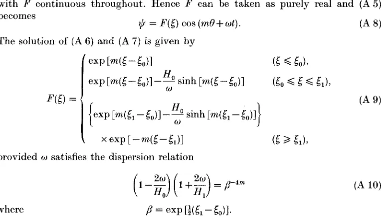
Each mode is concentrated above a single mountain and the disturbance propagates around this mountain with shallow water to its right. One mode for this is illustrated in figure 1. The other mode can be formed by rotating the figure by n. The amplitude of the motion varies with position having its maximum between the mountains. The phase speed varies also, being slowest between the mountains and fastest on the far side. As the frequencies of both modes are of equal magnitude, another normal mode is formed by any linear combination of these two waves. This degeneracy is broken by any inhomogeneity in the system, in particular by the presence of a third mountain (Jansons & Johnson 1988).
For a mountain and an equal and opposite dale (i.e. H , = - H o ) , both of which in
isolation support oscillations of frequency
$Ho,
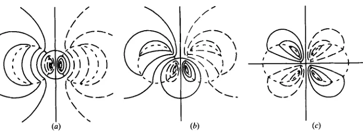
interaction splits the resonance to giveFigure 2 gives the streamline patterns for the higher frequency when disturbances propagating round the bottom contours are in phase. Figure 3 shows the patterns for the lower frequency when the disturbances are out of phase. Once again the disturbance is largest and slowest moving between the mountains. The existence of two close frequencies allows beating solutions, slowly transferring energy between the hill and the dale. Such solutions are discussed by Jansons & Johnson (1988).
P
= exp[%,
-to)].
(jJ =
*idO(
1-
p - 4 9(A
11)Topographic Rossby waves above a random array of seamountains 385
FIGURE 1. The streamline pattern for the lowest-order, dipole, mode concentrated over one of a pair of unit radius mountains of equal height. A second mode of the same frequency is obtained by rotating the figure by n. Negative values are dashed and bottom contours dotted. The patterns are shown a t one-eighth-period intervals. The sequence can thus be continued by appropriate reflections. The pattern succeeding ( c ) is given by reflecting ( b ) about the line of centres and changing signs. The pattern succeeding this is given by changing signs in (a) and so on. These illustrate the rapid propagation of phase on the far side of the mountain and the slower propagation between the mountains.
FIGURE 2. As in figure 1. but for a mountain and dale of equal and opposite height. These patterns are for the higher-frequency mode when disturbances propagating round the depth discontinuities are in phase.
\
\
,
/
/
386 K . M . Jansons and E .
R.
Johnson0.4
w
0.2
0.2 0.4 0.6 0.8 D
(4
FIGURE 4. The frequencies of the normal modes of two mountains of unit radius as a function of
D , their separation at nearest points scaled on a diameter. (a) The positive root for two mountains
of unit height for 0
<
D<
!. There is an equal and opposite negative root. ( i ) the limiting value a t infinite separation, w = $; (ii) the approximate form (A 15); (iii) the exact form (A 10). ( b ) As for(a) but for
a
<
D<
1. The vertical scale is highly magnified to show the exact form approaching the approximate before their joint approach to the limiting value. (c) The two roots for a mountain of unit height and a mountain of unit depth. The exact form approaches the approximate while both still differ significantly from the limiting value.For the case considered in the main text, of mountains of unit radius with centres separated by a distance d, say,
to
= -cosh-'(id),
= c0sh-l ( i d ) , a: = [($!)2- 11; (A 13)and
Thus
or
P = e x p ( & ) =$d+[(+d)2-1]6
Topographic Rossby waves above a random array of seamountains 387
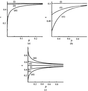
as obtained already for the dipole mode ( m = 1) in (28). Figure 4 ( a ) shows the positive root for o as a function of D, the distance between closest points expressed in diameters, for 0
<
D <a
for the dipole mode of two mountains of unit height. Curve (i) gives the value for w =t
for an isolated mountain, curve (ii) the approximate form (A 15), and curve (iii) the exact expression (A 13). By D = 0.01,an almost imperceptible separation, the frequency has already increased t o 60 YO of its limiting value. Figure 4 ( b ) gives the same curves for
a
<
D
<
1, on an expanded scale, showing by D = a difference of less than +YO between the approximate and exact values. The approach to the asymptotic form of higher modes (i.e. m 3 2) is even faster.For the case of resonance (i.e. H , = - H o ) , that is, a mountain and a dale,
w =
glo[
1f
d-2m+
O(d-"-2)],(A
16)which gives (29) for the dipole mode. Figure
4
( c ) shows the limiting, approximate and exact values of o as a function ofD.
The approach to the limiting value is slower in this case, but once again the approximate form is highly accurate, being within 1 %b y D = l .
Appendix B.
Two concentric circles
circles by the transformation The solution constructed in Appendix A is mapped into that for two concentric 7+ia = exp((+iB). (B 1)
For an inner circle of radius unity and an outer circle of radius a (so
6,
= O , g , = log aand /3 = a;), (A 10) becomes
as quoted for m = 1 in (57). This result can of course be derived directly using polar coordinates.
R E F E R E N C E S
BRETHERTON, F. P. & HAIDVOGEL, D. B. 1976 Two-dimensional turbulence above topography.
J . Fluid Mech. 78, 12S154.
GILL, A. E., DAVEY, M. K., JOHNSON, E. R. & LINDEN, P. 1986 Rossby adjustment over a step.
J . Mar. Res. 44, 713-738.
HIDE, R. 1961 Origin of Jupiter's Great Red Spot. Nature 190, 895-896.
JAMES, I. N. 1980 The forces due to geostrophic flow over shallow topography. Geophys.
JANSONS, K. M. & JOHNSON, E. R. 1988 Slow energy transfer between regions supporting
JOHNSON, E. R. 1984 Starting flow for an obstacle moving transversely in a rapidly rotating fluid.
JOHNSON, E. R. 1985 Topographic waves and the evolution of coastal currents. J . Fluid Mech.
JOHNSON, E. R. 1986 A conformal mapping technique for the topographic wave equation. JISAO
JOHNSON, E. R. 1987 A conformal mapping technique for the topographic wave equation - semi- Astrophys. Fluid Dyn. 14, 225-250.
topographic waves. J . Fluid Mech. (in press).
J . Fluid Mech. 149, 71-88.
160, 49S509.
Rep. 31, University of Washington.
388 K . M . Jansons and E .
R.
JohnsonLEBLOND, P. H. & MYSAK, L. A. 1978 Waves in the Ocean, chap. 5 . Elsevier Oceanography Series,
RIIINES, P. B. 1969 Slow oscillations in an ocean of varying depth. Part 2. Islands and seamounts.
TAYLOR, G. I. 1923 Experiments on the motion of solid bodies in rotating fluids. Proc. R. SOC.
TIIOMSON, R. E. 1975 The propagation of planetary waves over a random topography. J . Fluid
vol. 20. Elsevier.
J . Fluid Mech. 37, 191-205.
Lon,d. A 104, 213-218.