Optimization of Query Processing Time Base on
Materialized Sample View
Mahip Bartere and Dr. Prashant Deshmukh
Computer Science Department, Sipna College of Engineering and Technology,Amravati, Maharashtra, India.
Abstract-Sample views created from the database tables are
useful in many applications for reducing retrieval time. A sample view is an indexed materialized view that permits efficient sampling from an arbitrary range query over the view. Such “sample views” are very useful in applications that require random samples from a database: Approximate query processing, online aggregation, data mining, and randomized algorithms are a few examples. The Appendability, Combinability, and Exponentiality (ACE) Tree is a new file organization technique that is suitable for organizing and indexing a sample view. One of the most important aspects of the ACE Tree is that it supports online random sampling from the view. That is, at all times, the set of records returned by the ACE Tree constitutes a statistically random sample of the database records satisfying the relational selection predicate over the view.
Keywords- ACE Tree, Materialized View, Query Processing.
I INTRODUCTION
Database sampling has been recognized as an important problem that the International Organization for Standardization (ISO) has been working to develop a standard interface for sampling from relational database systems[1], and significant research efforts are directed at providing sampling from database systems by vendors such as IBM . However, despite the obvious importance of random sampling in a database environment and dozens of recent papers on the subject, there has been relatively little work toward actually supporting random sampling with physical database file organizations. The classic work in this area [by Olken and Rotem] suffers from drawback. With the ever-increasing database sizes, randomization and randomized algorithms[2] have become vital data management tools. In particular, random sampling is one of the most important sources of randomness for such algorithms. Scores of algorithms that are useful over large data repositories either require a randomized input ordering for data (i.e. an online random sample) or operate over samples of the data to increase the speed of the algorithm. For example, in online aggregation[3], database records are processed one at a time and are used for keeping the user informed of the current “best guess” as to the eventual answer to the query. If the records are input into the online aggregation algorithm in a randomized order, then it becomes possible to give probabilistic guarantees on the relationship of the current guess to the eventual answer to the query. Data mining algorithms like scalable K-Means[4] clustering and frequent item set mining are applicable only if the data are processed in a randomized order. In general, it is often possible to scale data mining and machine learning
techniques by incorporating samples into a learned model one at a time until the marginal accuracy of adding an additional sample into the model is small. Materialized views defined over distributed data sources are critical for many applications to ensure efficient access, reliable performance, and high availability. This work deals with efficient optimization of query with the help of materialized view over the distributed network. Materialized views need to be maintained upon source updates since stale view extents may not serve well or may even mislead user applications. Thus, view maintenance performance is one of the keys to the success of these applications [5].
There are several benefits of Materialized View such as • Less writes
• Decreased CPU consumption • Markedly faster response times • Less physical reads
• Materialized Views offer us flexibility of basing a view on Primary key
• Users, Applications, Developers and others can take advantage of the fact that the answer has already been stored for them. • Tools such as the DBMS_OLAP Package allow for easier
maintenance.
• In a read-only / read-intensive environment will provide reduced query response time and reduced resources needed to actually process the queries.
II PRESENT THEORIES AND PRACTICES
algorithm in a randomized order, then it becomes possible to give probabilistic guarantees on the relationship of the current guess to the eventual answer to the query. Data mining algorithms like scalable K-Means[4] clustering and frequent item set mining are applicable only if the data are processed in a randomized order. In general, it is often possible to scale data mining and machine learning techniques by incorporating samples into a learned model one at a time until the marginal accuracy of adding an additional sample into the model is small.
Materialized views defined over distributed data sources are critical for many applications to ensure efficient access, reliable performance, and high availability. This work deals with efficient optimization of query with the help of materialized view over the distributed network. Materialized views need to be maintained upon source updates since stale view extents may not serve well or may even mislead user applications. Thus, view maintenance performance is one of the keys to the success of these applications [5].
III SYSTEM ARCHITECHTURE
The materialized sample view can be used as a convenient abstraction for allowing efficient random sampling from a database. For example, consider the following database schema:
SALE (DAY, CUST, PART, SUPP) To support fast random sampling from this table, and most of queries include a temporal range predicate on the DAY attribute. This is exactly the interface provided by a materialized sample view. A materialized sample view can be specified with the following SQL-like query: CREATE MATERIALIZED SAMPLE VIEW MyVw AS SELECT * FROM SALE INDEX ON DAY.
Although the materialized sample view is a straightforward concept, an efficient implementation is difficult. The primary objective is to index data using properties Appendability, Combinability, and Exponentiality (ACE), which can be used for efficiently implementing a materialized sample view. The proposed work will be based on ACE tree traversal algorithm. The following issues will be considered in the dissertation work:
1. Initially two phases will be implemented. In the first phase the data set is sorted based on the record key values. This sorted order of records is used for providing the split points associated with each internal node in the tree. 2. In the second phase the data are organized into leaf nodes
based on those key values. Disk blocks corresponding to groups of internal nodes can easily be constructed at the same time as the final pass through the data writes the leaf nodes to the disk.
3. ACE trees can be extended to support the queries that include multidimensional predicates. K-d binary trees can be useful for that purpose instead of binary trees.
4. Instead of using simple arrays for storing node information other data structures can be useful to improve the performance of overall process.
Following flow chart shows how the execution takes place
F
Fig 1 . Architecture of system of query optimization
During the implementation, these views have the following characteristics.
1.It is possible to efficiently sample views (without replacement) from any arbitrary range query over the indexed attribute at a rate that is far faster than is possible by using other techniques or by scanning a randomly permuted file. In general, the view can produce samples from a predicate involving any attribute having a natural ordering, and a straightforward extension of the ACE Tree. Which can be used for sampling from multidimensional predicates. 2 .The resulting sample is online, which means that new samples
are returned continuously as time progresses and in a manner such that at all times, the set of samples returned is a true random sample of all of the records in the view that match the range query. This is vital for important applications like online aggregation and data mining.
3. Finally, the sample view created efficiently, requiring only two external sorts of the records in the view and with only a very small space overhead beyond the storage required for the data records.
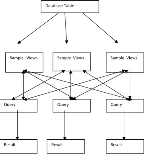
Initially user logs in to ACE processing system. Then selects the node for which sample views are to be created. The selection of node will be from the available node list. Then user will be connected to the database for which DSN’s are created for that node. Then user gathers all the tables available in the database. User selects a table. After selecting table ACE shows all fields in the table. Then user selects number of fields on which views are to be created. After user selects generate sample view. Now the sample views are generated using ACE algorithm. After generating sample views user can fire query using sample views or without using sample views. The appropriate results will be
Database Table
Query Query Query
Result
Result Result
Sample Views Sample Views
showed to user. The required for processing will be displayed to user and comparison will be carried out.
IV. ACE TREE AND MATERIALIZED VIEWS
We propose an entirely different strategy for implementing a materialized sample view. Our strategy uses a new data structure called the ACE Tree to index the records in the sample view. At the highest level, the ACE Tree partitions a data set into a large number of different random samples such that each is a random sample without replacement from one particular range query. When an application asks to sample from some arbitrary range query, the ACE Tree and its associated algorithms filter and combine these samples so that very quickly, a large and random subset of the records satisfying the range query is returned. The sampling algorithm of the ACE Tree is an online algorithm, which means that as time progresses, a much larger sample is produced by the structure. At all times, the set of records retrieved is a true random sample of all the database records matching the range selection predicate.
A. ACE TREE
Logically, the ACE Tree is a disk-based binary tree data structure with internal nodes used for indexing leaf nodes, and leaf nodes used for storing the actual data. Since the internal nodes in a binary tree are much smaller than disk pages, they are packed and stored together in disk-page sized units [19]. Each internal node has the following components: 1. A range R of key values associated with the node.
2. A key value k that splits R and partitions the data on the left and right of the node.
3. Pointers ptrl and ptrr, which point to the left and right children of the node.
4. Counts cntl and cntr, which give the number of database records falling in the ranges associated with the left and right child nodes. These values can be used during the evaluation of online aggregation queries, which require the size of the population from which we are sampling[4].
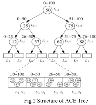
Fig. 2 shows the logical structure of the ACE Tree. Ii;j refers to the jth internal node at level i. The root node is labeled with a range I1,1.R =[0 – 100], signifying that all records in the data set have key values within this range. The key of the root node partitions I1,1.R into I2,1.R=[0–50] and I2,2.R=[51 – 100]. Similarly, each internal node divides the range of its descendents with its own key.
The ranges associated with each section of a leaf node are determined by the ranges associated with each internal node on the path from the root node to the leaf. For example, if we consider the path from the root node down to leaf node L4, the ranges that we encounter along the path are 0-100, 0-50, 26-50, and 38-50.
Thus, for L4, L4:S1 has a random sample of records in the range 0-100, L4:S2 has a random sample in the range 0-50, L4:S3 has a random sample in the range 26-50, whereas L4:S4 has a random sample in the range 38-50.
Fig 2 Structure of ACE Tree B. EXAMPLE OF ACE TREE
In the following discussion, we demonstrate how the ACE Tree efficiently retrieves a large random sample of records for any given range query. The query algorithm is formally described in next section.
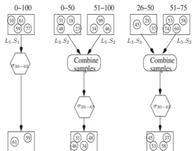
Let Q =[30 - 65] be our example query postulated over the ACE Tree depicted in Fig. 2. The query algorithm starts at I1,1, which is the root node. Since I2,1.R overlaps Q, the algorithm decides to explore the left child node labeled I2,1 in Fig. 2. At this point, the two range values associated with the left and right children of I2,1 are 0-25 and 26-50. Since the left child range has no overlap with the query range, the algorithm chooses to explore the right child next. At this child node I3,2, the algorithm picks leaf node L3 to be the first leaf node retrieved by the index. Records from section 1 of L3 (which totally encompasses Q) are filtered for Q and returned immediately to the consumer of the sample as a random sample from the range [30-65], whereas records from sections 2, 3, and 4 are stored in memory. Fig. 3 shows the one random sample from section 1 of L3, which can be used directly for answering query Q.
Next, the algorithm again starts at the root node and now chooses to explore the right child node I2,2. After performing range comparisons, it explores the left child of I2,2, which is I3,3, since I3,4.R has no overlap with Q. The algorithm chooses to visit the left child node of I3,3 next, which is leaf node L5. This is the second leaf node to be retrieved.
As depicted in Fig. 4, since L5.R1 encompasses Q, the records of L5.S1 are filtered and returned immediately to the user as two additional samples from R. Furthermore, section 2 records are combined with the section 2 records of L3 to obtain a random sample of records in the range 0-100.
Fig. 4. Combining samples from L3 and L5.
These are again filtered and returned, giving four more samples from Q. Section 3 records are also combined with the section 3 records of L3 to obtain a sample of records in the range 26-75. Since this range also encompasses R, the records are again filtered and returned, adding four more records to our sample. Finally, section 4 records are stored in memory for later use. Note that after retrieving just two leaf nodes in our small example, the algorithm obtains 11 randomly selected records from the query range. However, in a real index, this number would be many times greater. Thus, the ACE Tree supports “fast first” sampling from a range predicate: a large number of samples are returned very quickly. We contrast this with a sample taken from a B+-Tree having a similar structure to the ACE B+-Tree depicted in Fig. 2. The B+-Tree sampling algorithm would need to preselect which nodes to explore. Since four leaf nodes in the tree are needed to span the query range, there is a reasonably high likelihood that the first four samples taken would need to access all four leaf nodes. As the ACE Tree Query Algorithm progresses, it goes on to retrieve the rest of the leaf nodes in the order L4, L6, L1, L7, L2, and L8.
V PROPERTIES OF THE ACE TREE
In this section, we describe the three important properties of the ACE Tree, which facilitate efficient retrieval of random samples from any range query and will be instrumental in ensuring the performance of the algorithm, as described in algorithms.
A.COMBINABILITY
The various samples produced from processing a set of leaf nodes are combinable. For example, consider the two leaf nodes L1 and L3, and the query “Compute a random sample of the records in the query range Ql=[3 to 47].”
Fig. 5. Combining two sections of leaf nodes of the ACE tree.
As depicted in Fig. 5, first, we read leaf node L1 and filter the second section in order to produce a random sample of size n1 from Ql, which is returned to the user. Next, we read leaf node L3 and filter its second section L3.S2 to produce a random sample of size n2 from Ql, which is also returned to the user. At this point, the two sets returned to the user constitute a single random sample from Ql of size n1 þ n2. This means that as more nodes are read from the disk, the records contained in them can be combined to obtain an ever-increasing random sample from any range query.
B. APPENDABILITY
The ith sections from two leaf nodes are Appendable. That is, given two leaf nodes Lj and Lk, Lj.Si U Lk:Si is always a true random sample of all records of the database with key values within the range Lj.Ri U Lk.Ri. For example, reconsider the query “Compute a random sample of the records in the query range Ql=[3 to 47].”
As depicted in Fig. 6, we can append the third section from node L3 to the third section from node L1 and filter the result to produce yet another random sample from Ql. This means that sections are never wasted.
C. EXPONENTIALITY
The ranges in a leaf node are exponential. The number of database records that fall in L.Ri is twice the number of records that fall in L.Ri+1. This allows the ACE Tree to maintain the invariant that for any query Q’ over a relation R such that at least hµ database records fall in Q’, and with |R|/2k+1 <=|σQ’(R)| <=|R|/2k, V k<=h - 1, there exists a pair of leaf nodes Li and Lj, where at least half of the database records falling in Li.Rk+2 U Lj.Rk+2 are also in Q’. µ is the average number of records in each section, and h is the height of the tree or, equivalently, the total number of sections in any leaf node. Although the formal statement of the exponentiality property is a bit complicated, the net result is simple. There is always a pair of leaf nodes whose sections can be appended to form a set that can be filtered to quickly obtain a sample from any range query Q’. As an illustration, consider query Q over the ACE Tree in Fig.2. Note that the number of database records falling in Q is greater than 1/4 but less than half the database size. The exponentiality property assures us that Q can be totally covered by appending sections of two different leaf nodes. In our example, this means that Q can be covered by appending section 3 of nodes L4 and L6. If RC = L4R3 U L6.R3, then by the invariant given above, we can claim that |σQ(R)| >= (1/2) x |σRC(R)|.
VI DEVLOPMENT AND IMPLEMENTATION OF ALGORITHM
The algorithm has been designed to meet the primary goal of achieving “fast first” sampling from the index structure, which means that it attempts to be greedy on the number of records relevant for the query in the early stages of execution. In order to meet this goal, the query answering algorithm identifies the leaf nodes that contain the maximum number of sections relevant for the query. A section Li1.Sj is relevant for a range query Q if Li1.Rj U Q≠Φ, and Li1.Rj U Li2.Rj U . . . U Lin.Rj Q, where Li1 , . . . , Lin are some leaf nodes in the tree. The query algorithm prioritizes retrieval of leaf nodes so as to
facilitate the combination of sections so as to maximize n in the above formulation and
maximize the number of relevant sections in each leaf node L retrieved such that L.Sj∩Q≠Φ, where j =(c + 1) . . . h, where L.Rc is the smallest range in L that encompasses Q.
A. ALGORITHM OVERVIEW
At a high level, the query answering algorithm retrieves the leaf nodes that are relevant to answering a query via a series of stabs or traversals, accessing one leaf node per stab. Each stab begins at the root node and traverses down to a leaf. The distinctive feature of the algorithm is that at each internal node that is traversed during a stab, the algorithm chooses to access the child node that was not chosen the last time that the node was traversed. For example, imagine that for a given internal node I, the algorithm chooses to traverse to the left child of I during a stab. The next time that I is
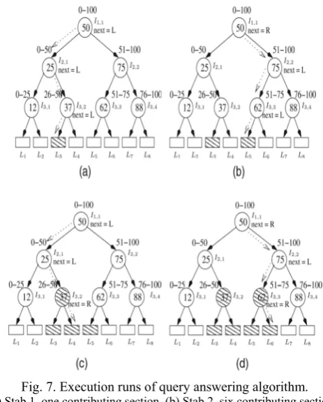
accessed during a stab, the algorithm will choose to traverse to the right child node. This can be seen in Fig. 7, where we compare the paths taken by stabs 1 and 2.
Fig. 7. Execution runs of query answering algorithm. (a) Stab 1, one contributing section. (b) Stab 2, six contributing sections.
(c) Stab 3,seven contributing sections. (d) Stab 4, 16 contributing sections.
The algorithm chooses to traverse to the left child of the root node during the first stab, whereas during the second stab, it chooses to traverse to the right child of the root node. The advantage of retrieving leaf nodes in this back-and forth sequence is that it allows us to quickly retrieve a set of leaf nodes with the most disparate sections possible in a given number of stabs. The reason that we want a non-homogeneous set of nodes is that nodes from very distant portions of a query range will tend to have sections covering large ranges that do not overlap. This allows us to append sections of newly retrieved leaf nodes with the corresponding sections of previously retrieved leaf nodes. The samples obtained can then be filtered and immediately returned.
accessed. In such a case, the internal node that overlaps the query range is not chosen and is never accessed again.In addition to the structure of the internal and leaf nodes of the ACE Tree, the query algorithm uses and updates two memory resident data structures:
1. A lookup table T. This is for storing internal node information in the form of a pair of values (next = [LEFT]|[RIGHT, done=[TRUE]|[FALSE]). The first value indicates whether the next node to be retrieved should be the left child or right child. The second value is TRUE if all leaf nodes in the sub tree rooted at the current node have already been accessed, else it is FALSE.
2. An array buckets[h]. This is for holding sections of all leaf nodes that have been accessed so far and whose records could not be used for answering the query. h is the height of the ACE Tree.
B. ACTUAL ALGORITHM
We now present the algorithms used for answering queries by using the ACE Tree. Algorithm 2 simply calls Algorithm 3, which is the main tree traversal algorithm, called Shuttle(). Each traversal or stab begins at the root node and proceeds down to a leaf node. In each invocation of Shuttle(), a recursive call is made to either its left or right child with the recursion ending when it reaches a leaf node. At this point, the sections in the leaf node are combined with previously retrieved sections so that they can be used for answering the query. The algorithm for combining sections is described in Algorithm 4. This algorithm determines the sections that are required to be combined with every new section s that is retrieved and then searches for them in the array buckets[]. If all sections are found, it combines them with s and removes them from buckets[]. If it does not find all the required sections in buckets[], it stores s in buckets[]. Algorithm 2: Query Answering Algorithm
Procedure Answer (Query Q) Let root be the root of the ACE Tree While (!T.lookup(root).done) T.lookup(root).done=Shuttle(Q,root); Algorithm 3 :ACE Tree Traversal Algorithm Procedure Shuttle (Query Q, Node curr_node) If(curr_node is an internal node)
left_node=curr_node→get_left_node(); right_node=curr_node→get_right_node(); If(left_node is done AND right node is done) Mark curr_node as done
Else if(right_node is not done) Shuttle (Q,right_node); Else if(left_node is not done) Shuttle (Q,left_node);
Else if (both children are not done) If (Q overlap only with left_node.R) Shuttle (Q,left_node);
Else if (Q overlap only with right_node.R) Shuttle (Q,right_node);
Else // Q overlaps both sides or none If (next node is LEFT)
Shuttle (Q,left_node); Set next node to RIGHT; If (next node is RIGHT)
Shuttle(Q,right_node); Set next node to LEFT; Else // curr_node is a leaf node Combine_Tuples(Q,curr_node); Mark curr_node as done
Algorithm 4: Algorithm for Combining Sections Procedure Combine_Tuples(Query Q,LeafNode node) For each section s in node do
Store the section numbers required to be Combined with s to span Q,in a list list For each section number I in list do If buckets does not have section i Flag=false
If(flag== true)
Combine all sections from list with s And use the records to answer Q Else
Store s in the appropriate bucket
C. ALGORITHM ANALYSIS
We now present a lower bound on the expected performance of the ACE Tree index for sampling from a relational selection predicate. For simplicity, our analysis assumes that the number of leaf nodes in the tree is a power of 2.
Lemma 1: Efficiency of the ACE Tree for Query Evaluation. Let n be the total number of leaf nodes in an ACE Tree,
which is used for sampling from some arbitrary range query Q.
Let p be the largest power of 2 not greater than n. Let _ be the mean section size in the tree.
Let _ be the fraction of database records falling in Q. Let N be the size of the sample from Q that has been
obtained after m ACE Tree leaf nodes have been retrieved from the disk.
If m is not too large (that is, if m≤ 2αn + 2), then
where E[N] denotes the expected value of N (the mean value of N after an infinite number of trials).
Proof. Let Ii,j and Ii,j+1 be the two internal nodes in the ACE Tree, where R = Ii,j.R U Ii,j+1.R covers Q, and i is maximized. As long as the Shuttle algorithm has not retrieved all the children of Ii,j and Ii,j+1 (this is the case, as long as m ≤ 2αn+2), when the mth leaf node has been processed, the expected number of new samples obtained is
Thus, after m leaf nodes have been obtained, the total number of expected samples is given by
If m is a power of 2, the result is proven.
Lemma 2. The expected number of records _ in any leaf node section is given by
where |R| is the total number of database records, h is the height of the ACE Tree, and 2h-1 is the number of leaf nodes in the ACE Tree.
Proof. The probability of assigning a record to any section i; i ≤ h is 1/h.
Given that the record is assigned to section i, it can be assigned to only one of 2i-1 leaf node groups after comparing with the appropriate medians. Since each group would have 2h-1 / 2i-1 candidate leaf nodes, the probability that the record is assigned to some leaf node Lj is
VII CONCLUSION
The selection of views to materialize is one of the most important issues in designing a database. So as to achieve the best combination of good query response where query processing view maintenance cost should be minimized in a given storage space constraints. The total cost, composed of different query patterns and frequencies, were evaluated for three different view materialization strategies. The total cost evaluated from using the proposed materialized-views method was proved to be the smallest among the three strategies. Further, an experiment was conducted to record different execution times of the proposed strategy in the computation of a fixed number of queries and maintenance processes. Again, the proposed materialized-views method requires the shortest total processing time.
REFERENCES
[1] Shantanu joshi and Christopher Jermaine “Materialized Sample Views For Database Approximation” IEEE transaction on knowledge and data engineering, march 2008..
[2] J.M. Hellerstein, P.J. Haas, and H.J. Wang, “Online Aggregation,” Proc. ACM SIGMOD, pp. 171-182, 1997.
[3]Bin Liu And Elke A. Rundensteiner, “Optimizing Cyclic Join View Maintenance Over Distributed Data Sources” IEEE Transactions On Knowledge And Data Engineering, Vol. 18, No. 3, March 2006.
[4] P.S. Bradley, U.M. Fayyad, and C. Reina, “Scaling Clustering Algorithms to Large Databases,” Proc. Third Int’l Conf. Knowledge Discovery and Data Mining (KDD ’98), pp. 9-15, 1998.
[5]Shantanu joshi and Christopher Jermaine “Materialized Sample Views For Database Approximation” ieee transaction on knowledge and data engineering, march 2008
[6] J.M. Hellerstein, P.J. Haas, and H.J. Wang, “Online Aggregation,” Proc. ACM SIGMOD, pp. 171-182, 1997.
[7]D.G. Severance and G.M. Lohman, “Differential Files: Their Application to the Maintenance of Large Databases,” ACM Trans. Database Systems, vol. 1, no. 3, pp. 256-267, 1976.