Article
1
Identifying the Frequency Dependent Interactions
2
Between Ocean Waves and The Continental Margin
3
on Seismic Noise Recordings
4
Zhen Guo 1, Yu Huang 1,2,*, Adnan Aydin 3 and Mei Xue 4
5
1 College of Civil Engineering, Tongji University, Shanghai 200092, China; [email protected]
6
2 Key Laboratory of Geotechnical and Underground Engineering of the Ministry of Education, Tongji
7
University, Shanghai 200092, China; [email protected]
8
3 Department of Geology and Geological Engineering, The University of Mississippi, University, MS 38677,
9
USA; [email protected]
10
4 State Key Laboratory of Marine Geology, Tongji University, Shanghai, 200092, China;
11
12
* Correspondence: [email protected];
13
Abstract: This study presents an exploration into identifying the interactions between ocean waves
14
and the continental margin in the origination of double-frequency (DF, 0.1-0.5 Hz) microseisms
15
recorded at 33 stations across East Coast of USA (ECUSA) during a ten-day period of ordinary ocean
16
wave climate. Daily primary vibration directions are calculated in three frequency bands and
17
projected as great circles passing through each station. In each band, the great circles from all
18
stations exhibit largest spatial density primarily near the continental slope in the western North
19
Atlantic Ocean. Generation mechanisms of three DF microseism events are explored by comparing
20
temporal and spatial variations of the DF microseisms with the migration patterns of ocean wave
21
fronts in Wavewatch III hindcasts. Correlation analyses are conducted by comparing the frequency
22
compositions of and calculating the correlation coefficients between the DF microseisms and the
23
ocean waves recorded at selected buoys. The observations and analyses lead to a hypothesis that
24
the continental slope causes wave reflection, generating low frequency DF energy and that the
25
continental shelf is where high frequency DF energy is mainly generated in ECUSA. The hypothesis
26
is supported by the primary vibration directions being mainly perpendicular to the strike of the
27
continental slope.
28
Keywords: ocean waves; double-frequency microseisms; continental margin; continental slope
29
30
1. Introduction
31
Ambient noise (or seismic noise) has been widely used to estimate the seismic site effect
32
parameters (e.g. predominant frequency f0, sediment thickness, amplification factor, etc.) of a site [1–
33
5] and to characterize both deep (down to the mantle of the Earth) and shallow (within the depth of
34
geological engineering activities) subsurface structures [6–15] for its advantages as a fast, effective
35
and reliable tool. However, the accuracies and reliabilities of the applications listed above would
36
strongly affected by the spatial and temporal variations of the ambient noise sources. One example
37
is given in [16] who estimated the amplification factors in Northern Mississippi of United States
38
applying the horizontal-to-vertical spectral ratio (HVSR, or Nakamura) method based on long term
39
ambient noise recordings. As the f0s in their study region lie in the frequency band of ocean waves
40
induced double frequency (DF) microseisms (0.1–0.5 Hz), the estimated amplification factors (HVSR
41
values at f0) fluctuate with time and are strongly correlated with the energy of the DF microseisms as
42
well as the ocean wave height. Many other studies suggest that if the noise sources are not
43
homogeneously distributed, the cross-correlation function cannot be reconstructed causing big errors
44
in subsurface tomography or even failure of subsurface tomography [17–22]. In addition, the ambient
45
noise with frequency greater than 0.1 Hz would be used in shallow subsurface tomography. From
46
this point of view, exploring the source locations, the spatial and temporal characteristics and the
47
generation mechanisms of the ambient noise with frequency greater than 0.1 Hz, especially the DF
48
microseisms, would significantly improve the application of the ambient noise in site effect
49
evaluation and shallow subsurface tomography.
50
In the spectrum of ambient noise recorded globally, the DF microseisms (or secondary
51
microseisms) manifest themselves as one or more energy peaks in the frequency band of 0.1–0.5 Hz
52
which is roughly twice of ocean waves’ frequencies. It is widely accepted that DF microseisms are
53
generated by the non-linear interaction between ocean waves propagating in opposite directions with
54
similar frequencies (e.g. [23–31]).
55
56
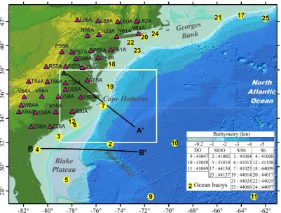
Figure 1. Study area and locations of transportable array (TA) stations (triangles) and NOAA buoys
57
(yellow circles), recordings of which are analyzed in this study. The table lists the original numbers
58
and a simplified numbering scheme of the ocean buoys grouped according to their four distinct
59
locations: deep ocean (DO), the continental slope-deep ocean side (SlDO), the continental slope-shelf
60
side (SlSh) and the continental shelf (Sh). The color-encoded relief base map is from [32]. The black
61
lines A-A’ and B-B’ are the transects presented in Figure 8a and 8b. The white box indicates the area
62
where the underground shear velocity model (Figure 8c and 8d) was computed based on [15].
63
Recent studies suggest that two different circumstances may be responsible for generating
64
opposing ocean waves. The first group considers wave-wave interactions in the open-ocean during
65
strong storms [27,33–35]. However, DF microseisms can be observed worldwide even when there are
66
no strong storms locally or globally. This is explained by the second group of studies who emphasize
67
the role of interactions between the ocean waves and the continental margin, i.e. the ocean waves
68
being reflected at the coastal lines [22,36,37]. For example, [38] observed that Rayleigh waves in a
69
microseism recording at an ocean bottom seismometer in Pacific Ocean were approaching from
70
California coast during a super-typhoon rather than the location of the typhoon and concluded that
71
the microseisms were generated by interactions of typhoon-induced waves toward and their
72
reflections from the coastal line. In a different set of studies based on correlation analyses between
the ocean storms developed close to shorelines and the ambient noise recorded on coastal seafloor or
74
costal land, it was recognized that the long- and short-period DF microseisms (LPDF, 0.085–0.2 Hz
75
and SPDF, 0.2–0.5 Hz respectively) were excited by swells from distant and local waves respectively
76
[25,30,31,39,40]. However, regarding the locations where the interactions (reflection) occur, there exist
77
a debate in terms of the water depth (deep or coastal). [41] summarized the debate and compared
78
theoretical and observed DF characteristics for each case considering the ocean wave frequency
79
composition and velocities. It appears that the relationship between DF microseisms and ocean waves
80
is not yet directly investigated as a function of water depth across the continental margin.
81
In this study, the continental slope, as a boundary between shallow (continental shelf) and deep
82
(open ocean) water, is explored for its interactions with the ocean waves as well as its role and
83
significance in the generation of DF microseisms. To reach this goal, the following data are utilized:
84
(a) a total of 10-days of ambient noise data recordings from 33 seismic stations (Figure 1) of
85
Transportable Array (TA) network along parts of the middle and southeastern North Atlantic coastal
86
area and the Shenandoah Valley, (b) the WAVEWATCH III® (WWIII) hindcasts of ocean wave
87
energy in Atlantic Ocean, and (c) ocean wave climate parameters recorded at relevant ocean buoys
88
by National Data Buoy Center (NDBC) in Atlantic Ocean. While the selected recording period is free
89
of major anomalous ocean activities (e.g. ocean storm, typhoon, hurricane) in Atlantic or Pacific
90
Oceans (according to National Hurricane Center, NHC), it includes a few examples of relatively
91
strong DF microseism events. Generation mechanisms of these events are explored by comparing
92
temporal and spatial variations of the PSDs with the migration patterns of ocean wave fronts in
93
WWIII hindcasts. For the entire period of microseism recordings, correlation analyses are conducted
94
by comparing the frequency compositions of and correlation coefficients between DF microseisms
95
and ocean wave parameters recorded at selected buoys.
96
2. Materials and Methods
97
2.1. Ambient noise data
98
The original time series in vertical (V), north-south (N) and east-west (E) directions are first
99
parsed into 1-hour segments, followed by removing the mean, linear trend and instrument response
100
in each segment [42]. Then each segment is processed following a 14-step procedure summarized
101
below, to estimate the power spectral density (PSD) in horizontal (H) and vertical (V) directions (steps
102
1 – 5), and the primary vibration direction by the radial-to-transverse spectral ratio (Ra) method (steps
103
6 – 10) as well as the polarization analysis method based on [43] (steps 11 – 14) in the three DF bands
104
(DF1, 0.1–0.2 Hz; DF2, 0.2–0.3 Hz; and DF3, 0.3–0.4 Hz). The two methods used to estimate the
105
primary vibration directions are both based on an assumption that DF microseisms propagate
106
dominantly as a fundamental mode Rayleigh wave [34,44–46]. The Ra method searches the direction
107
of the largest ratio of radial to transverse components on horizontal plane which is expected to be
108
along the propagation direction of Rayleigh wave [29,42]. The polarization analysis method
109
represents the particle motion within a short time range (when the propagation direction is
110
reasonably stable) as an ellipsoid with three axes perpendicular to each other [43], from which the
111
back azimuth of the major axis with highest probability for the whole recording period can be
112
calculated. If the primary energy source is stable and strong enough, and significantly larger than
113
secondary sources, the primary vibration directions obtained by the two methods would agree
114
because the secondary sources do not alter direction of major axis but increase the Ra values in
115
directions other than the major axis.
116
The steps of the data analysis are:
117
1. Apply an anti-triggering algorithm based on a prescribed range of short (1 s) to long (30 s) term
118
average amplitude ratios (0.2 < STA/LTA < 2.5) to filter each segment for avoiding occasional
119
energy bursts [4,47].
120
2. Apply fast Fourier transform with a 10% cosine taper on the filtered segments in three directions
121
to calculate spectra (𝑉(𝑓), 𝑁(𝑓), and 𝐸(𝑓)) and then smooth them using Konno-Ohmachi
122
method with a bandwidth coefficient of 40 [48].
3. Calculate the resultant horizontal spectrum (𝐻(𝑓)):
124
𝐻(𝑓) = ( ) ( ) , (1)
125
4. Compute the PSDs in vertical and resultant horizontal directions [49] in unit of (m/s2)2/Hz dB:
126
𝑃(𝑓) = 10 log
. ∙
∆
∙ 𝑌(𝑓) , (2)
127
where 𝑃(𝑓) and 𝑌(𝑓) are the PSD and spectral amplitude respectively in vertical or resultant
128
horizontal direction as function of frequency (f); 𝛥𝑡 is the sample interval (0.01s); N is the
129
number of samples in each selected time-series segment; the constant 1/0.825 is a scale factor to
130
correct for the 10% cosine taper applied [50].
131
5. Plot the PSDs of all segments at each station in time-frequency domain 𝑃𝑆𝐷(𝑡, 𝑓).
132
6. Apply band-pass filter using the frequency bands, F = 0.1–0.2 Hz (DF1), 0.2–0.3 Hz (DF2) and
133
0.3–0.4 Hz (DF3) to each 1-hour segment to produce filtered amplitude-time series 𝑉(𝑡, 𝐹),
134
𝑁(𝑡, 𝐹), and 𝐸(𝑡, 𝐹).
135
7. Rotate the two horizontal components by an angle φ into radial (R) and transverse (T)
136
components [51] in each segment:
137
𝑅(𝑡, 𝐹, 𝜑)
𝑇(𝑡, 𝐹, 𝜑) =
−cos (𝜑) −sin (𝜑)
−sin (𝜑) −cos (𝜑)
𝑁(𝑡, 𝐹)
𝐸(𝑡, 𝐹) , (3)
138
in which φ is defined as the back-azimuth angle between the north and the radial direction from
139
the recording station toward the source.
140
8. Calculate the root mean square of 𝑅(𝑡, 𝐹, 𝜑) and 𝑇(𝑡, 𝐹, 𝜑) in each segment and their ratio
141
𝑅𝑎(𝐹, 𝜑).
142
9. Repeat steps 7 and 8 to calculate 𝑅𝑎(𝐹, 𝜑) at every 1° increment of angle φ in 1°-360°.
143
10. Calculate average values of 𝑅𝑎(𝐹, 𝜑) for all segments at a station and determine the azimuth
144
𝜑 for the maximum value of these averages. The angle 𝜑 is taken as the primary vibration
145
direction by 𝑅𝑎 method.
146
11. Further parse the filtered 1 hour segments in step 6 into ten 120 s windows and determine 𝑉 ,
147
𝑁 , 𝐸 , where i = 1, 2 and 3 (separating DF1, DF2 and DF3 contents) and j = 1, 2, …, 30 (number
148
of windows). For each window, build the three-component covariance matrix M:
149
𝐌𝒊𝒋=
𝑐𝑜𝑣 𝑉 , 𝑉 𝑐𝑜𝑣 𝑉 , 𝑁 𝑐𝑜𝑣 𝑉 , 𝐸
𝑐𝑜𝑣 𝑁 , 𝑉 𝑐𝑜𝑣 𝑁 , 𝑁 𝑐𝑜𝑣 𝑁 , 𝐸
𝑐𝑜𝑣 𝐸 , 𝑉 𝑐𝑜𝑣 𝐸 , 𝑁 𝑐𝑜𝑣 𝐸 , 𝐸
, (4)
150
12. Calculate the three eigenvalues 𝜆 and associated eigenvectors 𝑥⃗ of the covariance matrix
151
𝐌𝒊𝒋 by solving:
152
𝐌𝒊𝒋𝑥⃗ = 𝜆 𝑥⃗ , (5)
153
and define the maximum eigenvalue 𝜆 , and associated eigenvectors (𝑥 𝑥 𝑥 )⊺.
154
13. Find the back azimuth angle 𝜑 corresponding to the major axis of the polarized ellipse:
155
𝜑 = arctan 𝑖𝑓 𝑥 > 0
𝜑 = arctan + 180 𝑖𝑓 𝑥 < 0, (7)
156
14. Compute the probability of the back azimuth angle within 0°-360° range with a 10° bin width.
157
The back azimuth of highest probability is considered as the primary vibration direction by the
158
polarization method.
159
2.2. Ocean data
160
Theoretically, the frequencies of ocean waves that generate DF microseisms should be half of the
161
frequencies of DF peaks. Therefore, daily WWIII hindcast of E(F/2) (log10(m2/Hz)) distributions within
162
the half frequency bands of corresponding DF peaks are used in this study in order to explore the
163
association between the ocean wave climates in Northern Atlantic Ocean and DF microseisms.
164
Additionally, a total of 19 ocean buoys in Atlantic Ocean (see Figure 1 for locations) are selected to
165
retrieve recordings of the ocean climate parameters including dominant wave period and significant
166
wave height (detailed descriptions of which can be found at NDBC website). In order to clearly display
167
the locations of the buoys on the figure and to facilitate discussion of the observations, these buoys are
renumbered and divided into four groups according to their locations (Figure 1): 1) deep ocean (DO)
169
buoys (9, 10 and 11); 2) the continental slope and deep ocean side (SlDO) buoys (2, 5, 17 and 25); 3) the
170
continental slope and shelf side (SlSh) buoys (3, 6, 7, 19, 21 and 23); and 4) the continental shelf (Sh)
171
buoys (the remaining ones).
172
In order for a direct comparison of frequency compositions of the ocean wave and DF microseisms,
173
the dominant ocean wave frequency of ocean waves at each buoy is simply doubled to determine the
174
double ocean wave frequency (DWF).
175
3. Results
176
3.1. Power spectral density (PSD)
177
178
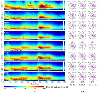
Figure 2. (a) Power spectral density (PSD) plots in time-frequency domain of the vertical components
179
at the selected stations. The dashed lines at 0.2 and 0.3 Hz mark the boundaries of the three frequencies
180
ranges. Three relatively strong DF microseism events are identified and labeled as I, II and III. (b)
181
Polar plots of average 𝑅𝑎(𝜑) values (blue) combined with rose diagrams of back azimuths
182
(calculated by the polarization analysis) (purple) at the three DF bands at the selected stations in the
183
whole recording period. On each plot, the text labels refer to the recording station (e.g. N61A), central
184
frequency of DF peak (e.g. 0.17 Hz), probability of back azimuth (in purple, e.g. 10%) and the scale of
185
the solid outer circle in multiples of the 𝑅𝑎(𝜑) value (in blue, e.g. Ra = 2). Same plots for the
186
remaining stations are shown in Figure S1 in the supplement materials.
187
Figure 2a shows the vertical PSD(t,f) plots at the stations selected to cover a wide latitude range
188
(40°N ~ 34°N) (see Figure 1 for locations of the stations). The remaining stations are divided into three
189
groups according to their locations (for their groups, see Figure S1a in the Supplementary Materials
to this article) and their 𝑃𝑆𝐷(𝑡, 𝑓) plots are shown in Figure S1b, S1d and S1f. In the recording time
191
period of this study, DF peaks are mainly in frequency band of 0.15 – 0.3 Hz at the selected example
192
stations, however, may cover a much wider frequency band at the stations close to the coastline (see
193
Figure S1b in the Supplementary Materials to this article). At all stations, three DF microseism events
194
with relatively high energy levels are identified and labeled with I, II and III which will be described
195
in section 3.3. Since DF microseisms exist continuously, clear starting and ending times for such
196
events cannot be determined precisely, which are therefore taken as the boundaries of high PSD level
197
periods (Figure 2a).
198
3.2. Primary vibration directions at DF peaks
199
Figure 2b presents the polar plots of average radial-to-transverse spectral ratios Ra(φ) (blue
200
outline) and rose diagrams of back azimuths calculated by the polarization analysis (purple) in DF1,
201
DF2 and DF3 bands for the selected stations over the entire recording period of 10 days. The same
202
plots for the remaining stations are given in Figures S1c, S1e and S1g in supplementary materials.
203
The longer axis of each 𝑅𝑎(𝜑) outline is identified indicating the average primary vibration direction
204
in ten days (𝜑 ), which closely coincide with the major polarized direction.
205
The daily primary vibration directions (𝜑 ) are calculated as well for all stations, and rose
206
diagrams of them in ten days are generated for the three DF bands in Figure 3. The main
back-207
azimuth in the three DF bands are shown to be in 110°–150°, which is perfectly consistent with the
208
results in the same area in [52].
209
210
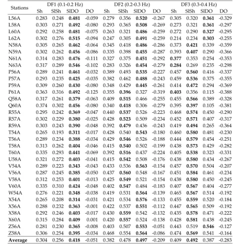
Figure 3. The normalized spatial density (color gradient maps) of the great circles corresponding to
211
the daily primary vibration directions (𝜑 ) and the vertical PSDs averaged for the entire recording
212
period (scaled circles) in the three DF bands. The yellow lines contour the density of 0.5. The
rose-213
diagram shows the probability distribution of all 𝜑 s.
214
The great circles corresponding to all 𝜑 are generated in the three DF bands. Any point on a
215
great circle can be considered as a possible energy source of the corresponding station in the
216
corresponding day and DF band. In order to find the possible source areas, spatial density of the
217
points sampled from the great circles with a sampling interval of 100 m are calculated, normalized
218
and plotted as color gradient map for each DF band in Figure 3, as well as the contours at density of
219
0.5 and the ocean bathymetries. The relative magnitude of the spatial density reflects the possibility
220
of the area to be energy source, i.e. the larger the density, the higher the possibility. Comparing the
221
three maps, it can be observed that the areas of high spatial density, e.g. the areas sketched by the
222
density contours of 0.5, shrink towards the continental shelf with increase of frequency, and the
223
spatial density in the area between Blake Ridge and Cape Hatteras is high in all three DF bands.
224
First, the spectral WWIII hindcasts of ocean wave energy (E(F/2) in log10(m2/Hz)) in North
226
Atlantic Ocean (see Figure S2 in the Supplementary Materials to this article) are used to explore the
227
temporal and spatial relationships in each frequency band of the energy levels between PSDs and
228
wave energy. This analysis demonstrates that 1) the primary vibration directions do not point to the
229
areas of high wave energy in open ocean, and 2) variations of ocean wave activities in open ocean of
230
North Atlantic Ocean have limited influence on the DF microseisms observed in east coast of United
231
States.
232
Based on the spatial density of great circles presented in Figure 3, it can be inferred that the
233
excitations of DF microseisms appear to be associated with the ocean waves in different areas of the
234
continental margin of the western North Atlantic Ocean. Therefore, the excitation mechanisms of the
235
three DF microseism events identified in Figure 2 are explored below with reference to area of the
236
continental margin as outlined in Figure 4.
237
238
Figure 4. (a), (c) and (d) Daily WAVEWATCH III hindcasts of ocean wave spectra (E(F/2) in
239
log10(m2/Hz)) in Northern Atlantic Ocean (color gradient maps), PSD levels (small circles with scaled
240
sizes) and primary vibration directions (segments of great circles) at all stations corresponding to the
241
three events (I, II and III) identified in Figure 2. The purple circles/ellipses delimit the intersections of
242
the great circles; (d), (e) and (f) Time history of average PSDs in three frequency bands. In each plot,
243
the curves are stacked by the latitudes of the stations and the relief of each curve shows the change
244
of PSD level. The starting time of the three events are picked and connected to form the red lines, the
245
arrows of which show the impact sequence.
246
Figures 4a, 4c and 4e show the WWIII hindcasts of E(F/2) in the western Northern Atlantic Ocean
247
(color gradient maps) within the half frequency band of events I, II and III identified in Figure 2. In
248
the corresponding days and frequency bands of the events, the PSD levels and the primary vibration
249
directions are demonstrated by the small circles with scaled sizes and segments of great circles
250
passing though the corresponding stations. The bathymetries of the western Northern Atlantic Ocean
are plotted as well in order to examine the importance of the continental slope in generation of DF
252
microseisms. In Figures 4b, 4d and 4f, the arrival times of each event are picked on the PSD-time plots
253
of all stations, and the connection of them form the red lines indicating the sequence of energy impact
254
on stations. In order to facilitate the description of the spatial variations of PSD levels and primary
255
vibration directions, the area where stations are placed are divided into two sections, north and south
256
of Cape Hatteras.
257
3.3.1. Event I
258
The energy of event I in DF1 band (LPDF, 01-0.2 Hz) starts to appear on late hours of day
259
2014/325 (red line on day 325 in Figure 4b) and reaches a higher strength on days 2014/326 and 327
260
(Figures 2 and 4b). The ocean waves in frequency band of 0.05-0.1 Hz in deep ocean close to the
261
continental slope are uniformly higher on day 326 than day 327, and extend to the continental slope
262
(Figure 4a). In addition, intersections of great circles concentrate at several small areas (purple circles)
263
evenly distributed on the continental slope on day 326. All these observations might explain the
264
occurrence of event I at the same time on day 326. The ocean wave energy decreases in the deep ocean
265
close to the continental slope and increase slightly at the deep ocean area south of Georges Bank on
266
day 327. The primary vibration directions at all stations cover a wider range, and the intersections of
267
great circles are not as concentrated as on day 326. These changes can explain the decrease of PSD
268
levels at most stations except for eight northernmost stations on day 327.
269
3.3.2. Event II
270
The event II in DF2 (0.2-0.3 Hz) band occurs on days 2014/327, 328 and 329, and arrives at the
271
stations in south section before north section as indicated by the curved red arrow in Figure 4d. This
272
sequence can be explained by the ocean wave interactions associated with the continental slope
273
(Figure 4c).
274
On day 327, the wave energy in frequency band of 0.1-0.2 Hz are relatively higher on lower Blake
275
Plateau (water depth 200-2000 m) and many great circles of the stations in south section intersect on
276
the edge of this area. The PSD levels at the stations in south section are roughly proportional to their
277
distances to lower Blake Plateau. Then on day 328 the wave front moves north along the continental
278
slope to south of Cape Hatteras while the wave energy increases to the highest. The great circles of
279
almost all stations in south section intersect in this area, and the PSD levels at these stations increase
280
significantly. On day 329, the wave front moves further north to the area between Georges Bank and
281
Cape Hatteras where the strike of the continental slope turns almost 90 degrees, causing the
282
significant increase of wave energy in this area. The great circles at the stations in north section do
283
not intersect in the open ocean where the wave energy are higher, but on the continental slope
284
segments south of Georges Bank and north of Cape Hatteras. The PSD levels at the stations to the
285
north increase but not as significantly as at the southern stations on day 328. The great circles at the
286
southern stations still intersect at the continental slope between Cape Hatteras and Blake Plateau but
287
not as concentrated as on day 328.
288
3.3.3. Event III
289
The event III in DF2 (0.2-0.3 Hz) band occurs on days 2014/330, 331 and 332, arrives at the stations
290
almost at the same time, but generates the energy peaks slightly earlier at the stations in south section
291
(Figure 4d). This sequence can also be explained by the ocean wave interactions associated with the
292
continental slope (Figure 4e).
293
On day 330, the great circles of most stations point to the area between Georges Bank and Blake
294
Plateau where the ocean waves are roughly in same height, and intersect evenly on this continental
295
slope segment. But the ocean wave energy on the continental slope of Georges Bank are relatively
296
higher which coincide well with the relatively higher PSD levels at the four northernmost stations.
297
On day 331, the ocean wave energy grows very fast while the wave front moves north quickly to
298
Georges Bank, resulting in high waves on the continental slope segment and deep ocean area between
Georges Band and Blake Ridge. Most intersections of the great circles align on this continental slope
300
segment and nearby deep ocean, and the PSD levels are very high at all stations. On day 332, the
301
wave front moves to northeast of Georges Bank and the wave energy decreases moderately.
302
However, the wave energy on the continental slope south of Georges Bank is still relatively high and
303
many great circles of the stations in northern section intersect here, which might be the reason of high
304
PSD levels at the eight northernmost stations. A new high wave front is developed at Blake Ridge
305
where most great circles of stations in southern section intersect, and a new PSD peak appears at the
306
stations in southern section.
307
3.4. Correlation between DF microseisms and ocean wave parameters
308
Table 1. Average correlation coefficients (CC) between the PSDs in the three DF bands and the
309
ocean wave heights in four groups of ocean buoys.
310
Stations Sh DF1 (0.1-0.2 Hz) SlSh SlDO DO Sh DF2 (0.2-0.3 Hz) SlSh SlDO DO Sh DF3 (0.3-0.4 Hz) SlSh SlDO DO L56A 0.283 0.248 0.481 -0.059 0.279 0.356 0.520 -0.267 0.305 0.320 0.361 -0.329 L58A 0.303 0.271 0.492 -0.080 0.293 0.365 0.508 -0.269 0.273 0.321 0.361 -0.297 L60A 0.292 0.258 0.481 -0.075 0.263 0.321 0.486 -0.259 0.272 0.290 0.327 -0.295 L62A 0.302 0.276 0.515 -0.094 0.247 0.305 0.491 -0.259 0.214 0.234 0.303 -0.255 N58A 0.305 0.265 0.462 -0.064 0.345 0.418 0.486 -0.286 0.373 0.421 0.339 -0.359 N59A 0.302 0.262 0.456 -0.086 0.335 0.398 0.455 -0.287 0.393 0.407 0.290 -0.366 N61A 0.314 0.283 0.476 -0.111 0.327 0.375 0.451 -0.292 0.377 0.353 0.254 -0.353 N63A 0.317 0.289 0.546 -0.102 0.283 0.326 0.454 -0.279 0.284 0.269 0.235 -0.298 P56A 0.289 0.241 0.461 -0.032 0.389 0.493 0.535 -0.227 0.457 0.560 0.416 -0.337 P57A 0.293 0.235 0.425 -0.035 0.382 0.462 0.488 -0.243 0.459 0.536 0.375 -0.355 P59A 0.309 0.260 0.430 -0.080 0.348 0.429 0.445 -0.261 0.414 0.472 0.294 -0.369 P61A 0.363 0.316 0.492 -0.125 0.355 0.396 0.327 -0.319 0.403 0.356 0.115 -0.388 Q58A 0.317 0.261 0.379 -0.063 0.409 0.515 0.466 -0.255 0.455 0.566 0.389 -0.328 Q60A 0.374 0.302 0.456 -0.080 0.340 0.418 0.306 -0.279 0.395 0.397 0.105 -0.381 R55A 0.295 0.242 0.369 -0.047 0.440 0.537 0.526 -0.223 0.468 0.574 0.450 -0.290 R57A 0.302 0.229 0.380 -0.025 0.428 0.523 0.509 -0.234 0.452 0.571 0.407 -0.317 R59A 0.303 0.243 0.390 -0.048 0.392 0.479 0.436 -0.243 0.419 0.494 0.265 -0.364 T54A 0.265 0.193 0.311 -0.017 0.428 0.540 0.543 -0.180 0.460 0.580 0.481 -0.230 T56A 0.289 0.234 0.388 -0.034 0.429 0.546 0.526 -0.188 0.444 0.579 0.454 -0.251 T58A 0.313 0.262 0.404 -0.046 0.415 0.540 0.502 -0.199 0.438 0.573 0.429 -0.282 T60A 0.335 0.293 0.441 -0.069 0.392 0.516 0.437 -0.224 0.405 0.538 0.323 -0.331 U58A 0.321 0.272 0.403 -0.041 0.415 0.542 0.508 -0.176 0.438 0.580 0.434 -0.267 V54A 0.289 0.223 0.343 -0.043 0.433 0.536 0.563 -0.154 0.457 0.570 0.504 -0.207 V56A 0.287 0.245 0.385 -0.050 0.437 0.560 0.548 -0.167 0.451 0.584 0.461 -0.234 V58A 0.312 0.253 0.401 -0.013 0.425 0.549 0.521 -0.154 0.438 0.580 0.450 -0.245 V60A 0.335 0.310 0.424 -0.048 0.402 0.547 0.484 -0.183 0.407 0.567 0.404 -0.277 W54A 0.276 0.221 0.348 -0.038 0.419 0.531 0.564 -0.139 0.465 0.567 0.514 -0.192 X54A 0.265 0.208 0.314 -0.031 0.421 0.534 0.576 -0.133 0.455 0.559 0.520 -0.184 X56A 0.288 0.232 0.363 -0.001 0.422 0.537 0.551 -0.112 0.447 0.565 0.509 -0.192 X58A 0.292 0.246 0.403 -0.017 0.430 0.559 0.542 -0.132 0.435 0.578 0.471 -0.222 X60A 0.315 0.284 0.409 0.001 0.420 0.557 0.524 -0.138 0.428 0.581 0.438 -0.245 Z56A 0.281 0.230 0.365 -0.008 0.403 0.507 0.553 -0.051 0.443 0.519 0.546 -0.127 Z58A 0.306 0.254 0.395 -0.034 0.468 0.554 0.564 -0.086 0.474 0.569 0.541 -0.164
Average 0.304 0.256 0.418 -0.051 0.382 0.478 0.497 -0.209 0.409 0.492 0.387 -0.283
In order to investigate the significance of the continental slope in the excitation of the DF
311
microseisms quantitatively, correlation analyses of time histories between DF microseisms and ocean
312
wave parameters recorded at the selected buoys in four groups (DO, SlDO, SlSh and Sh in Figure 1)
313
are carried out by considering the time-dependent variation of frequency composition and energy
314
levels.
315
The time histories of average PSDs in DF1, DF2 and DF3 bands are shown in Figures 4b, 4d and
316
4f respectively. The curves are stacked according to the latitudes of the stations and the reliefs show
317
the time-dependent variations of PSD levels. The double ocean wave frequencies (DWF) at the DO,
318
SlDO and SlSh buoys are closer to the frequency band of event I, and the waves whose DWFs match
319
events II and III are observed in groups SlDO, SlSh and Sh (for the time history of DWFs at the buoys,
320
see Figure S3 in the Supplementary Materials to this article). The correlation coefficients (CC) between
321
the time series of ocean wave height and PSD in the three DF bands are calculated for all pairs of
322
ocean buoy and ambient noise station, and the CC values are then averaged in each buoy group for
323
each DF band at each station, as summarized in Table 1. The bottom row of Table 1 gives the CC
324
values averaged for all stations. The CC values are normalized within the range [-1.0, 1.0], where
325
positive (negative) values represent same (opposite) trends of ocean wave height and PSD pairs and
326
the absolute value of CC express the level of consistency in these trends. In the DF1 band, better
327
correlations can be found between the DF microseisms at all stations and the ocean wave heights in
328
the continental slope on deep ocean side (SlDO). In the DF2 band, the DF microseisms at most stations
329
correlate well with the ocean wave heights in SlDO, and some with those in the continental slope on
330
shelf side (SlSh). In the DF3 band, higher CC values can be found in all SlDO, SlSh and continental
331
shelf (Sh) groups. Near-zero negative CC values for the deep ocean (DO) buoys implies that deep
332
ocean waves do not exert a positive influence on the DF microseisms.
333
4. Discussion
334
4.1. Hypothesis on the significance of continental slope for the origination of DF microseisms
335
The correlation analysis (Table 1) shows that the DF microseism trends in DF1, DF2 and DF3
336
bands are most compatible with the ocean wave activities in the continental slope on deep ocean side
337
(SlDO), the continental slope on both deep ocean and continental shelf sides (SlDO and SlSh), and
338
SlSh respectively. These domains of wave activities are separated by the continental slope, where
339
waves approaching from the deep ocean zone are reflected back creating non-linear wave-wave
340
interactions. This naturally leads to a hypothesis that the continental slope plays a significant role in
341
the origination of DF microseisms, and with increasing frequency band, the dominant origination
342
area migrates from SlDO to SlSh in east coast of United States. Validity of this hypothesis is explained
343
in detail in the following.
344
During the time period of event I (Figure 4a), the continental slope is shown to be the boundary
345
of impact from the ocean wave in frequency band of 0.05–0.1 Hz, the increase of wave energy in deep
346
ocean area south of Georges Bank does not cause increase of PSD levels at the stations in north section
347
but the decrease of ocean wave energy on the continental slope do coincide well with the decrease of
348
PSD levels in most stations from day 2014/326 to 327. Comparing events II and III (Figures 4c and 4e),
349
the PSD levels are much higher on day 331 than day 329, mainly because the higher wave energy on
350
the continental slope between Georges Bank and Blake Ridge on day 331. Figure 5 shows the
351
differences of the wave energy and PSD levels corresponding to DF2 band between day 331 and 329.
352
A coincidence can be found between the changes of PSD levels and wave energy on the continental
353
slope segment between the Georges Bank and Blake Ridge (outlined by the purple dash-dot line),
354
which supports the hypothesis.
355
Because no hurricane development was reported in Northern Atlantic Ocean during the period
356
of recordings analyzed in this study, most DF microseisms identified from these recordings should
357
be generated mainly by the non-linear interactions of incoming and reflected ocean waves of similar
358
frequencies. These interactions take place at different intensities and directions as determined by
359
ordinary ocean activities and ocean bottom topography. Theoretically strong reflections leading to
strong DF energy can occur only if the incoming waves encounter an obstacle perpendicular to their
361
propagation direction, as shown in Figure 6. The area and energy of constructive interaction is much
362
larger when the incoming wave direction is perpendicular (Figure 6b) than nearly parallel (Figure 6a)
363
to the obstacle. Considering that, in a reflection system, at each point of incidence at any angle, the
364
energy normal to the reflector is the largest (Figure 6b), a station receives strongest signal when the
365
station and incident point is aligned with the line normal to the reflector (Path A in Figure 6b). Such
366
an alignment should therefore correspond to the great circles (lines connecting the wave origination
367
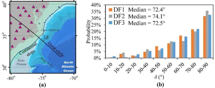
areas to the stations) intersecting the continental slope nearly at orthogonal angles. In order to test
368
this hypothesis, the intersection angles 𝜹 between the great circles and the strike of the continental
369
slope are defined as shown in Figure 7a and the frequency histograms of 𝜹s in the three DF bands
370
are generated and shown in Figure 7b. The medians of 𝜹s in the three DF bands are 72.4°, 74.1° and
371
72.5° respectively, and the largest frequencies of occurrences are within 81°-90° range, which support
372
the proposed hypothesis.
373
374
Figure 5. Difference of the ocean wave energy (E(F/2) in log10(m2/Hz)) and PSD levels between day
375
329 and 331 (Figure 4c and 4e respectively).
376
377
Figure 6. A sketch describing how constructive interactions of ocean waves and their reflections from
378
a barrier (the continental slope or the shoreline) can result in different energies when the angle of
379
incidence is (a) large and (b) 0°. Note a given station receives the strongest signals along the shortest
380
path A.
381
As the waves are reflected from the continental slope, the wave energy should be higher in the
382
continental slope and the nearby deep ocean zone than in the distant deep ocean zone and the
383
continental shelf. To examine this notion, the mean and standard deviation of ocean wave energy are
384
calculated in each of the four buoy groups, 2.19 and 0.44 m in DO, 2.48 and 0.98 m in SlDO, 2.10 and
385
0.99 m in SlSh and 1.57 and 0.74 m in Sh. The highest wave energy appears at the SlDO buoys and
then DO and SlSh buoys, which coincide well with areas of intersection of the great circle paths
387
(purple dashed ellipses in Figure 4). Similar observations can also be found in [33]. Recalling once
388
more that there was no strong storm in the northern Atlantic Ocean during the microseism
389
recordings, the identified DF microseisms cannot be explained by ocean storms.
390
391
Figure 7. (a) Defining the angle 𝛿 (< 90°) between a great circle and the continental slope’s strike, (b)
392
Histogram of the angles 𝛿s in the three DF bands.
393
The hypothesis is also supported by several ocean bottom observations in shallow and deep
394
waters divided by the continental slope. For example, [53] concluded that the excitation at DF peaks
395
require some part of the ocean storm to extend over the shallow water based on coherence studies.
396
Comparing ocean waves recorded in shallow waters (100 m deep) in Tasman Sea and microseisms
397
recorded near shoreline (30 km away from the ocean buoy) of North Island of New Zealand, [54]
398
observed that DF peaks were in > 0.2 Hz band when there was a local wind in the Tasman Sea but
399
lower than 0.2 Hz when the sea was calm and a swell from Southern Ocean arrived across the
400
continental slope. Another example is presented by [31]. Two pressure spectra were obtained from
401
two seafloor stations in the continental shelf (water depth of 0.6 km) and in the continental shelf edge
402
followed by a steep and deep continental slope (water depth of 1 km) respectively off the coast of
403
southern California (see topographic profiles in [55]). At the shallower site, a high spectral peak with
404
pressure level of around 103 Pa2/Hz was observed at around 0.2 Hz when a storm directly passed
405
overhead, whereas no spectral peak could be clearly identified when there was no passing storm. On
406
the deeper site, two high and sharp pressure spectral peaks appeared at 0.14 and 0.3 Hz with pressure
407
levels of 5×10³ and 104 Pa2/Hz respectively. Differences between the effects of shallow and deep ocean
408
on DF peaks’ frequencies and energy levels presented in these studies imply that DF microseism in
409
the continental shelf is driven by local weather, whereas that in the deep ocean is excited by the
410
standing waves [35] generated by the interaction between the distant ocean swell and the waves
411
reflected due to the sudden change of water depth at the continental slope.
412
4.2. Types of continental margin
413
In this study, two types of continental margins are identified as exemplified by the transects
A-414
A’ and B-B’ (profile locations are marked in Figure 1) in Figure 8a and 9b respectively. Both types
415
have wide (~100 km) and shallow (< 0.2 km) shelves. Along the first type (A-A’), a high (~2.5 km) and
416
steep slope sharply change the profile followed by a long gentle slope (continental rise). In the second
417
type (B-B’), the shelf transition into the slope via a wide and gently dipping plateau (Blake Plateau)
418
followed by a shorter (~1.5 km) and gentler slope (than the first type), then a wide undulating plateau
419
(continental rise) ending with a relatively steep slope.
420
These differences between the continental margin profiles appear to modify the mechanism of
421
DF microseism generation as suggested by the consistently high spatial densities in the area covering
422
the Blake Ridge and northern Blake Plateau in all three DF bands (Figure 3). A more gradual
423
transition from the shelf and a shorter continental slope are the most prominent features that can
424
support generation of a relatively stable energy level in these areas. Concavity of the continental slope
at the edge of Blake Plateau potentially causes strong reflections resulting in higher DF energy. In
426
contrast, the continental slope at Cape Hatteras has a convex outline that could cause a diffraction
427
pattern, consequently a lower spatial density in this area as shown in the map of DF1 band in Figure
428
3. As the DF3 microseisms are generated in the continental shelf, the rough shoreline at Cape Hatteras
429
may be the reason for higher density observed in DF3 band in Figure 3.
430
431
Figure 8. Topographic profiles of the continental margin along (a) A-A’ and (b) B-B’ (marked in Figure
432
1) based on General Bathymetric Chart of the Oceans (GEBCO, 2014). The shear velocity profile and
433
contours in (a) are based on [15]. The geophysical interface between sediments and bedrock is
434
estimated (black dotted line) by HVSR method and was extended seaward by inference (black dashed
435
line) to connect with the 2.2 km/s shear velocity contour. A transitional zone (TZ) with the largest
436
shear velocity gradient is identified and outlined by the two pink dashed lines in (a). The shear
437
velocity models inside the white box outlined in Figure 1 are generated for elevations (Elv.) of -5.2
438
km (c) and -15.2 km (d) based on [15].
439
Recent studies also support the hypothesis about the role of the continental slope and show that
440
submarine ridges act similarly to cause reflection of the waves. [56] by comparing the seasonal
441
variation of DF microseisms and ocean activities concluded that DF microseism in 0.15 – 0.2 Hz band
442
on the King George Island (on Antarctic Peninsula) originates from a region of Drake Passage instead
443
of the continental shelf around Antarctic Peninsula even though it is several times wider than that
444
around Cape Hatteras. The ocean at Drake Passage is at least 3 km deep and is delimited by the
445
continental slope of Antarctic Peninsula and an underwater ridge roughly normal to the slope. [33]
446
showed that the excitation locations of both P- and S-wave microseisms observed by a seismometer
447
array in Japan are distributed along the eastern continental slope of Greenland and Reykjanes Ridge
448
extended from Iceland into the deep ocean. An ocean bottom straight blocked by relief features [34,56]
449
promotes formation of ocean wave reflection at the continental slope.
450
The hypothesis may appear to fail the test based on the observations in [57], who compared the
451
DF spectra (around 0.15 Hz) at three seismometer stations in the coastal region of Oregon and
452
California with the ocean wave climate parameters’ spectra (see their figure 17). Based on an excellent
453
correlation between DF peak and wave spectra, they concluded that DF microseism is generated by
454
the wave activities near the shoreline. Significantly different widths of the continental shelves, being
455
much narrower on the western continental margin of North America, and the location of the ocean
buoys being on the edge of such a narrow continental shelf (see their figure 15) can explain the
457
apparent failure. Together with the low frequency (< 0.2 Hz) of their DF peak, it can be argued that
458
DF microseism observed by [57] was also a result of the reflections from the nearby continental slope
459
as put forward in the proposed hypothesis.
460
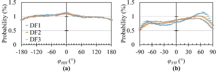
4.3. Rayleigh wave refraction
461
As mentioned in “Data acquisition and processing” section, the Ra and polarization analysis
462
methods to estimate the primary vibration direction are based on an assumption that DF microseisms
463
propagates dominantly as fundamental mode Rayleigh waves. To verify this assumption, Figure 9 is
464
generated to show the probability distributions of the phase differences between the two orthogonal
465
horizontal components (𝝋𝑯𝑯) and between the vertical and horizontal components on the primary
466
vibration direction (𝝋𝑽𝑯) in the three DF bands. The facts that 𝝋𝑯𝑯 is dominant in 0° and 𝝋𝑽𝑯 is
467
mainly in 65°– 80° and -65°– -80° reveal that the energy is propagating as Rayleigh waves dominantly
468
[58], which coincides well with the observation in [52].
469
470
Figure 9. Probability distribution of the phase difference between (a) the two horizontal components
471
(𝝋𝑯𝑯) and (b) the vertical and horizontal component on primary vibration direction (𝝋𝑽𝑯).
472
4.3.1. Refraction at the water-solid earth interface
473
As explained by [59], when the energy in the DF band is generated from wave-wave interaction
474
in the ocean, it propagates as “pseudo-Rayleigh waves” (pRg) in water column and turns to free
475
surface Rayleigh waves (FSRW) when it reaches solid earth. In the water column, due to phase speed
476
difference, the pRg exists in different forms: dominantly elastic pRg in shallow water with phase
477
speed roughly equal to that of FSRW, and acoustic pRg in deep water with phase speed of about 60%
478
of FSRW. Definitions of shallow and deep waters vary with the wave frequencies. According to the
479
analysis in this study, the energy in LPDF (DF1) band is generated around the continental slope
480
where the water depth is generally smaller than 3000 m (Figure 1), especially on Blake Plateau (≤ 1000
481
m) and edge of Blake Ridge (~3000 m). According to figure 14 in [59], with the increase of frequency
482
from 0.1 Hz to 0.2 Hz, the depth in the water column of elastic pRg dominance decrease from 3000 m
483
to 1500 m, under which the elastic pRg transfer to fundamental acoustic pRg. Thus, phase-speed
484
difference might exist at the water-solid earth interface deeper than 1500 m, i.e. areas except Blake
485
Plateau, however, the DF energy would still propagate vertically in the water column and transfer to
486
solid earth. Even though there is significant energy loss at the interface, the spherical spreading of
487
the DF energy in the solid earth will not change. Therefore, the phase speed difference on the
water-488
solid earth interface is not likely to affect the determination of source location by great circle. For
489
high-frequency (0.2–0.5 Hz) DF band, the hypothesis put forward in this manuscript claims that the
490
energy is generated in the continental slope and continental shelf where the water depth is smaller
491
than 200 m. The same figure in [59] shows that the energy in this band should also propagate as elastic
492
pRg and directly transition to FSRW on the continental shelf. Because there is no significant phase
493
speed difference between elastic pRg and FSRW, Rayleigh wave refraction at the surface of solid earth
494
is not likely to be significant.
495
4.3.2. Refraction within the solid earth
The Rayleigh wave ray paths are expected to bend also when they travel through the solid earth
497
boundaries with significant impedance contrasts. In order to examine possibility of such boundaries
498
and implications for the validity of the triangulation method, the shear velocity (Vs) structure of the
499
study area is explored as described below.
500
The cross section A-A’ presented in Figure 8a shows under the continental slope, there exists a
501
layer of material having Vs less than 2.2 km/s, which is interpreted as sediments in [15]. Our HVSR
502
survey around the eastern foothills of the Appalachian mountain and near the coastal area suggest
503
that the sediment-hard layer interface lies at a depth as depicted by a dotted line in the A-A’ profile
504
in Figure 8a, and that the average Vs of the sediment is about 0.9 km/s [5]. According to [48], the shear
505
velocity contrast at the sediment-hard layer interface should be larger than 2.5 to produce a clear a
506
predominant frequency peak on HVSR spectrum, therefore, the Vs of the hard layer should be around
507
2.2 km/s. Therefore, this interface is inferred to connect to the 2.2 km/s contour line (depicted as the
508
dashed line in Figure 8a). Shear velocity gradients are calculated along A-A’ at two different
509
elevations by [15] shear velocity model, and a transitional zone (TZ) of largest shear velocity gradient
510
(where Vs increases from about 1.7 to 3.2 km/s within a horizontal distance of ~80 km) is identified
511
and outlined as shown in Figure 8a. The TZ at Cape Hatteras (Figure 8c) extend roughly parallel to
512
the continental slope. The absence of notable shear velocity variations at -15.2 km (Figure 8d) suggests
513
that the transitional zone may not extend to this depth.
514
As explained above, the Rayleigh waves propagating through the solid earth from the deep
515
ocean near the continental slope (DF1 and DF2 bands) or from the continental shelf (DF3 band) to the
516
inland stations are expected to change propagation direction due to gradual and continuous
517
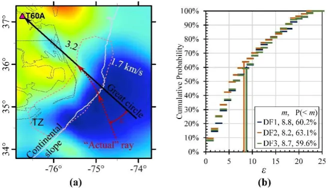
refraction as they pass through TZ. The total refraction angle ε is defined as shown in Figure 10a only
518
for the great circles passing through TZ which represents the worst scenario of changes. The
519
cumulative probability of ε in the three DF bands is given in Figure 10b. The weighted average (m)
520
of ε in DF1, DF2 and DF3 bands are calculated to be 8.8°, 8.2° and 8.7° respectively, and the
521
probabilities of ε values less than these corresponding weighted averages (P < m) are 60.2%, 63.1%
522
and 59.6%.
523
524
Figure 10. (a) Defining angle ε to measure total refraction of Rayleigh wave ray passing through the
525
transitional zone (TZ in Figure 8a and 8c). The black solid and red dotted lines are the great circle
526
projected in this study and “actual” ray path of Rayleigh wave respectively. b) Cumulative
527
probability of ε for waves in the three DF bands propagating through TZ.
528
Another examination of the Rayleigh wave refraction from sediments to bedrock is carried out
529
by tracking hurricane “Sandy” in Atlantic Ocean on 27 October 2012 using 8 hours ambient noise
530
recorded on the bedrock in Tishomingo, Mississippi. DF peak is found at the central frequency of 0.18
531
Hz with very high energy. The primary vibration direction at this central frequency is calculated by
532
both Ra and Polarization analysis methods and projected as great circles which point to the locations
533
of hurricane “Sandy” successfully (see Figure S4 in the Supplementary Materials to this article). Thus
the great circles can be considered as valid projections to the source areas of the DF energy.
535
4.3. Rayleigh wave refraction
536
According to the hypothesis and the discussion above, the DF microseisms in LPDF (DF1) band
537
is generated in the deep ocean close to the continental slope and propagate to stations on land.
538
Depending on the location of the stations, the propagation paths are different, i.e. through sediments
539
and bedrock to stations on inland bedrock, and through sediments on coastal stations on sediments,
540
resulting in different attenuations and energy levels at stations. This difference is observed in this
541
study. In Figure 3, the PSD levels in DF1 band increase from coast (sediments) to inland (Appalachian
542
Mountain) while the distance to source (ocean) increase. The possible explanation is that the
543
attenuation due to spherical spreading is less effective than energy absorption in sediments. A similar
544
trend is observed by [52] in the same study area. In DF2 band, the PSD levels at coastal stations are
545
slightly larger than or equal to those at inland stations, which might because the attenuation due to
546
spherical spreading and absorption in sediments are equally effective. In DF3 band, the PSD levels at
547
coastal stations are obviously larger than those at inland stations, due to the attenuation is
548
dominantly spherical spreading and absorption effect is equally effective, which reveals that the DF
549
microseisms in this band is generated in continental shelf and propagates mainly in sediments.
550
5. Conclusions
551
This study explored the role and significance of the continental slope in the interactions between
552
the ocean waves and the continental margin as well as the resulted double-frequency (DF)
553
microseisms recorded in ENAM. The primary vibration direction analysis of the ambient noise
554
recordings in the study area shows that these DF microseisms originated in areas of the North
555
Atlantic Ocean, which are generally aligned in SE direction with the recording stations. The great
556
circles corresponding to these primary vibration directions for different DF peaks intersect at a
557
number of locations enabling delineation of source areas along the continental slope. Correlation
558
analysis between DF microseisms and ocean wave climate by considering the correspondence in their
559
frequency composition and variation in energy levels shows that the DF microseisms in DF1 (0.1–0.2
560
Hz), DF2 (0.2–0.3 Hz) and DF3 (0.3–0.4 Hz) bands correlate well with the ocean wave activities in the
561
continental slope on deep ocean side, and in the continental slope on both deep ocean and shelf sides,
562
and in the continental slope on the shelf side respectively. These analyses lead to a hypothesis on the
563
frequency dependent interactions of ocean waves with the continental margin and the origination of
564
DF microseisms. The steep continental slope is a key submarine topographic feature which behaves
565
as an obstacle causing reflections of the incoming low frequency (≲ 0.15 Hz) ocean waves and
566
formation of standing waves to generate low frequency (≲ 0.3 Hz) DF microseisms. While the high
567
frequency (≳ 0.15 Hz) ocean waves are reflected at the shallow portion of the continental shelf to
568
excite high frequency (≳ 0.3 Hz) DF microseisms. This hypothesis is also supported by the
569
observations that 1) the great circles corresponding to the primary vibration directions of DF
570
microseisms are mostly normal to the strike of the continental slope; and 2) the ocean wave energy
571
in the continental slope or the nearby deep ocean are higher than in the distant deep ocean and the
572
continental shelf. Additional systematic observations at different parts of the globe will help to
573
determine validity and limits of the proposed hypothesis under all possible climatic and bathymetric
574
conditions.
575
With the frequency dependent interactions between the ocean waves and the continental margin
576
determined, one could further analyze the possible mass wasting on the continental margin caused
577
by the ocean wave energy input and transmission while ocean waves interact with the continental
578
margin.
579
Supplementary Materials: The following are available online at www.mdpi.com/xxx/s1, Figure S1: a) Map of
580
the USarray transportable array stations and their groups. Vertical power spectral density (PSD) plots in time
581
and frequency domain of b) coastal stations, d) Appalachian mountain stations, and f) south section stations. c),