Article
1
Surface-wave extraction based on morphological
2
diversity of seismic events
3
Xinming Qiu1, Chao Wang2,*, Jun Lu3 and Yun Wang4
4
1 School of Geophysics and Information Technology, China University of Geosciences (Beijing), Beijing,
5
China
6
2 The State Key Laboratory of Ore Deposit Geochemistry, Institute of Geochemistry, Chinese Academy of
7
Sciences, Guiyang, China
8
3 Key Laboratory of Marine Reservoir Evolution and Hydrocarbon Accumulation Mechanism, Ministry of
9
Education, China University of Geosciences (Beijing), Beijing, China
10
* Correspondence: [email protected]; Tel.: +86-156-5268-8034
11
12
Abstract: Extraction of high-resolution surface waves is essential in surface-wave survey. Because
13
reflections usually interfere with surface waves on X component in a multicomponent seismic
14
exploration, it is difficult to extract dispersion curves of surface waves. The situation goes more
15
serious when the frequencies and velocities of higher-mode surface waves are close to those of
PS-16
waves. A method for surface-wave extraction is proposed based on the morphological differences
17
between reflections and surface waves. Frequency-domain high-resolution linear Radon transform
18
(LRT) and time-domain high-resolution hyperbolic Radon transform (HRT) are used to represent
19
surface waves and reflections respectively. Then, the sparse representation problem based on the
20
morphological component analysis (MCA) is built and optimally solved to obtain high-fidelity
21
surface waves. An advantage of our method is its ability to extract surface waves when their
22
frequencies and velocities are close to those of reflections. Furthermore, results of synthetic and field
23
examples confirm that the proposed method can attenuate the distortion of surface-wave dispersive
24
energy caused by reflections, which contributes to extracting accurate dispersion curves.
25
Keywords: Higher-mode surface waves; dispersion curves; morphological component analysis;
26
Radon transform27
28
1. Introduction29
Seismic surface waves are widely used in crustal and mantle structure studies and engineering
30
prospecting, characterized by small horizontal attenuation, high signal-to-noise ratio and dispersion
31
[1, 2]. Dispersion characteristics of surface waves reflect the near-surface S-wave velocity structure.
32
Dispersion curves of fundamental-mode surface waves are inverted to obtain near-surface S-wave
33
velocity structure for PS-wave static corrections in a seismic exploration [3, 4]. Recently, considering
34
different sensitivity of fundamental- and higher-mode surface waves to elastic properties and
35
thickness of near-surface materials, joint inversion of fundamental- and higher-mode surface waves
36
is of wide-spread interest for less ambiguity and higher accuracy of S-wave velocities in engineering
37
seismic prospecting, ambient seismic noise tomography and microtremor survey [5-8]. To obtain
38
accurate S-wave velocities, extracting accurate dispersion curves of multi-mode surface waves is
39
essential.
40
Fundamental-mode surface waves are dominated in vertical-component seismic data while
41
higher-mode surface waves are generally evident on horizontal component or X component in a 2D
42
survey [9]. Disturbed by reflections, it is usually difficult to extract accurate dispersion curves of
43
higher-mode surface waves from X-component seismic data, causing the ambiguity of inverted
S-44
wave velocities. Luo et al. [10] proposed high-resolution LRT to image surface-wave dispersive
45
energy, which improved resolution of phase velocities. But disturbed by body waves or strong noise,
46
the dispersive energy may not be smooth and it is hard to distinguish between different modes,
47
known as “mode kissing” [11]. This phenomenon is vulnerable to mode misidentification [12],
48
resulting in less reliable inversion or even wrong inverted S-wave velocities.
49
To extract dispersion curves, surface waves are extracted on the basis of different characteristics
50
between surface waves and interference waves. Methods of surface-wave suppression are based on
51
single-component processing or multicomponent processing. Methods of single-component
52
processing include f-k filtering, empirical mode decomposition and other transform methods [4,
13-53
15] while methods of multicomponent processing are polarization filtering and vector median
54
filtering which preserve the vector characteristics and the spectral bandwidth of reflections [16, 17].
55
Pan et al. [18] discriminated the direct waves and reflections using frequency analysis. Performing a
56
hybrid linear-hyperbolic Radon transform, Trad et al. [19] separated surface waves successfully in
57
the signal model which consisted of both surface waves with linear events and reflections with
58
hyperbolic events. But raw data are transformed into the conventional intercept-slowness (τ-p)
59
domain, which is not sparse enough to separate surface waves in consideration of their dispersion
60
characteristics. Using high-resolution LRT, Hu et al. [20] transformed raw data into the
frequency-61
velocity (f-v) domain to implement surface-wave separation. However, it may be difficult to extract
62
surface waves in some cases dispersive energy of higher-mode surface waves also overlaps with that
63
of reflections in the f-v domain and then original surface-wave dispersive energy is distorted. Because
64
the frequencies and velocities of PS-waves are close to those of higher-mode surface waves [16].
65
In this paper, we propose a method of surface-wave extraction to overcome the influence of
66
reflections. The proposed method is based on the morphological differences between reflections and
67
surface waves. We also exploit the advantages of wavefield separation by frequency-domain LRT
68
and time-domain HRT. To implement surface-wave extraction, the sparse representation problem
69
under the framework of MCA is optimally solved.
70
We firstly describe the sparse representation problem and the selected sparse dictionaries,
71
followed by the distortion of surface-wave dispersive energy caused by reflections. Then, we
72
demonstrate the results of surface-wave extraction and picked dispersion curves using tests with
73
synthetic and field shot data.
74
2. Methods
75
2.1. Method of surface-wave extraction in f-v domain
76
High-resolution LRT is used to image surface-wave dispersive energy [10]. Using it, surface
77
waves and reflections on Z component are clearly in different locations of f-v domain when the
78
frequencies and velocities of them are significantly different. Hu et al. [20] extracted surface waves
79
from Z component by a 2D window of the f-v domain.
80
The frequency-domain inverse LRT in the matrix-vector form is [18]:
81
( )
=
( ) ( )
d
f
L
f
m
f
(1)where
d
( )
f
is a vector of size nx×1 representing the Fourier coefficients of the seismic data at82
the given frequency
f
whilem
( )
f
is a vector of sizenp
×
1
representing the Fourier83
coefficients of Radon panel at the given frequency
f
. In equation (1),L
( )
f
is a complex matrix of84
size
nx np
×
1 2 1 1 1 1 2 2 2 2 1 2 2 2 2 2 2 2 2 2 2
( )
π π π π π π π π π − − − − − − − − −
=
L
np np nx nx p n n x i fx i fx i fxv
v v
i fx i fx i fx
v
v v
i fx i fx i fx
v
v v
e
e
e
e
e
e
f
e
e
e
(2)
where
v
i(i 1,2,..., )
=
np
is the apparent velocity andx j
j(
=
1, 2,..., )
nx
is the offset.86
The frequency-domain high-resolution forward LRT [10, 21] is inverted with a sparse constraint
87
of a priori probability, known as:
88
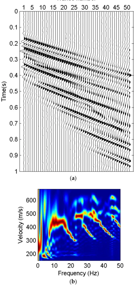
(
λ
I W L W W LW
+
−H H H −1)
m W L W W d
=
−H H Hm d d m m d d (3)
where
m W m
=
m .W
d is a matrix of data weights, a diagonal matrix showing the standard89
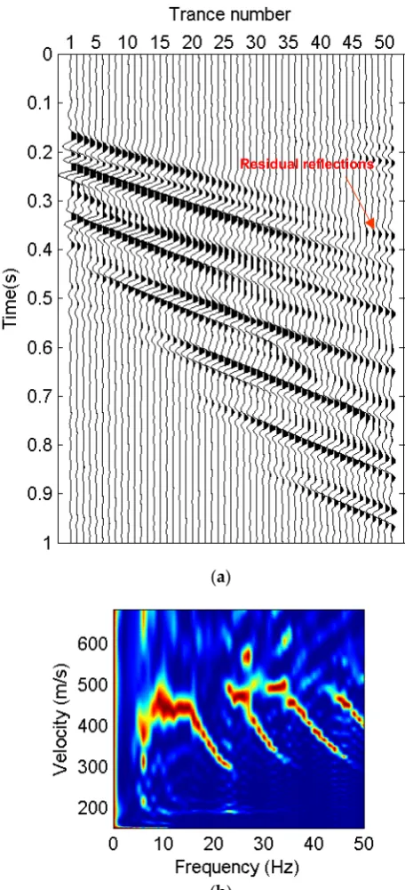
deviation,
diag(
W
d)
i=
( -
d Lm
)
i −1/2 whileW
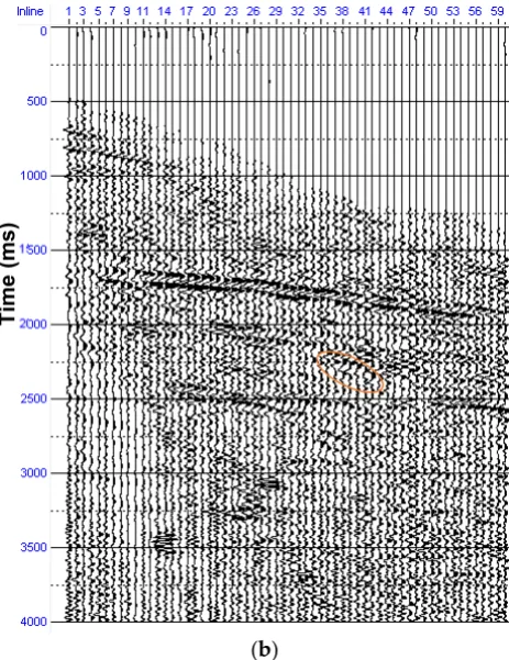
m is a diagonal matrix of Radon coefficients90
indicating how sparse the coefficients are,
diag(
W
m)
i=
m
i−1/2.I
denotes the identity matrix and91
the scalar λ is the tradeoff parameter that weights the relative importance of the misfit and the
92
sparsity [22].
93
But it is difficult to extract surface waves correctly from X-component seismic data. Because
94
frequencies and velocities of higher-mode surface waves and PS-waves are close and both of them
95
are generally evident on X component. Disturbed by PS-waves, the dispersive energy is not true for
96
surface waves. So, extracting surface waves in f-v domain is not a perfect method. We propose a
97
method of surface-wave extraction to overcome the influence of reflections based on MCA.
High-98
resolution LRT is one of two transforms and used to represent surface waves.
99
2.2. Sparse representation problem based on MCA
100
MCA is a method for signal separation based on sparse representations [23, 24]. It is assumed
101
that the original signal is a linear mixture of several different parts and for each of them, there exists
102
a dictionary which enables its construction using a sparse representation. Also, the dictionary can
103
only sparsely represent the corresponding part rather than others. For seismic data consisting of
104
surface waves and reflections, there is
105
g
+
r=
y y
y
(4)where
y
is the seismic data set,y
g is the surface-wave part andy
r is the reflection part. We106
choose
D
g andD
r as the sparse representation dictionaries of surface waves and reflections107
respectively, i.e.,
y
g=
D z
g g ,y
r=
D z
r r . Separation of surface waves and reflections can be108
formulated as [25]:
109
{
g r}
g g
2
r r 2 g 1 r 1 ,
1
argmin
(
2
−
−
+
μ
+
)
z z
y D z
D z
z
z
(5)where
z
g andz
r are the representation vectors for surface waves and reflections, respectively,110
and
μ
is the regularization parameter.111
Surface waves are generally modeled as broom-like events characterized by low frequency, low
112
velocity and dispersion, and their dispersive energy is around theoretical dispersion curves in the
f-113
v domain [20, 26]. Therefore, frequency-domain high-resolution LRT can sparsely represent surface
114
waves in theory. Reflections are approximated by hyperbolas and time-domain high-resolution HRT
can sparsely represent reflections with assumptions that velocities change little horizontally and
116
reflection interfaces are almost horizontal [27]. We choose frequency-domain high-resolution LRT
117
and time-domain high-resolution HRT to represent surface waves and reflections respectively. To
118
match with the matrix definition of sparse representation dictionaries in our sparse representation
119
problem, the inverse LRT and inverse HRT correspond to the matrix signs
D
g andD
r120
respectively while the forward LRT and forward HRT are respectively the matrices
D
g+ andD
r+.121
The matrices
D
g+ andD
r+ are pseudo inverse of the representation dictionaries, i.e.,z
g=
D y
g+ g,122
r
=
r+ rz
D y
. Put these back into (5) we obtain123
{
g r}
g r
2
2 g g
, 1 r r 1
1
argmin
2
μ
(
y
)
+ +
−
−
+
+
y y
y y
y
D
D
y
(6)which is solved by generalized BCR algorithm [23].
124
Surface waves is extracted by solving equation (6). Different dictionaries are respectively chosen
125
to represent surface waves and reflections so that the influence of reflections on surface-wave
126
dispersive energy is reduced.
127
2.2.1. Frequency-domain high-resolution LRT
128
To sparsely represent surface waves, equation (3) is solved to achieve high-resolution LRT in the
129
spectral bandwidth of surface waves by iteratively reweighted least squares (IRLS) algorithm [28].
130
The choice of the apparent-velocity range and interval should avoid aliasing [29] for reconstruction;
131
moreover, the apparent-velocity range includes the phase velocities of surface waves.
132
2.2.2. Time-domain high-resolution HRT
133
Inverse and adjoint HRT in the discrete form can be expressed as [30]:
134
( )
,
(
2 2/
2,
)
v
d t x
=
m
τ
=
t
−
x v v
(7)and
135
( )
(
2 2 2)
adj
,
/ ,
x
m
τ
v
=
d t
=
τ
+
x v x
(8)where
d t x
( )
,
are the seismic data in time-offset domain,x
indicates the offset,t
donatestwo-136
way time,
m
( )
τ
,
v
are the Radon coefficients,v
indicates the root-mean-square velocity of a137
reflection,
τ
donates the time intercept,m
adj( )
τ
,
v
are the low resolution Radon coefficients.138
Equations (7) and (8) are represented in matrix-vector form as follows [30]:
139
=
d Lm
(9)adj
=
m
L d
T(10) where
d
is a vector of sizeN
×
1
whose elements are taken trace-wise from the seismic data (140
= ×
N nx nt
) andm
is a vector of sizeM
×
1
whose elements are taken velocity-wise from the141
Radon coefficients (
M nv n
= ×
τ
).nx
,nt
,nv
andn
τ
are the number of traces, samples,142
velocities and time intercepts respectively. In equation (9) and (10), the operators
L
andL
T are143
just represented for the summation algorithms shown in equation (7) and (8) instead of matrices [31].
144
High-resolution forward HRT can be inverted from equation (9) using a sparse constraint
145
satisfying
146
1 1
(
W W
T)
−L W W Lm
T T=
(
W W
T)
−L W W d
T Twhich is solved by a left preconditioned version of conjugate gradient for the normal equations
147
algorithm [31].
148
The computational cost of applying operators
L
andL
T is controlled by the size of the149
Radon domain [32]. To speed up the implementation, time-domain high-resolution forward HRT is
150
solved in the restricted Radon space [32]
151
1 1
(
W W
T)
−L W W L m
T T=
(
W W
T)
−L W W d
T Tm m d d m m d d (12)
where
d
should be normalized to unity by dividing the maximum of the seismic data [33]. The152
restricted Radon space is defined as
153
( )
adj1
,
:
τ
=
>
p
nx
m
T
(13)where
T
is the threshold satisfying0
< <
T
1
.154
2.2.3. Performance of sparse representations using LRT and HRT
155
We synthesized the surface waves (Figure 1) of the two-horizontal-layer model (Model 1)
156
described by Table 1 using a staggered-grid finite-difference method. Then we synthesized reflections
157
(Figure 2) of the three-horizontal-layer model (Model 2) described by Table 2 using ray tracing.
158
Frequency-domain high-resolution forward LRT and time-domain high-resolution forward HRT are
159
applied to the surface waves and reflections to get the four panels of the Radon coefficients. Next, we
160
respectively normalized the Radon coefficients to unity divided by the maximum of each panel and
161
apply hard threshold to them. Finally, the seismic data were reconstructed by the inverse transforms.
162
For a Radon panel, the higher threshold amplitude means the fewer Radon coefficients used in the
163
reconstruction.
164
To confirm the effectiveness of sparse representations for surface waves and reflections, the
165
reconstruction error is calculated as follows:
166
0
=
r
x x
x x
err
E
E
(14)where
E
xr represents the root-mean-square error between reconstruction and original data at the167
offset
x
, i.e., xr=
1
(
( , )
−
( , )
)
2t
E
d t x
d t x
nt
,d t x
( , )
represent the reconstruction data, and168
(
)
20
=
1
( , )
x
t
E
d t x
nt
represents the root-mean-square value of original data at the offsetx
, i.e.,169
(
)
20
=
1
( , )
x
t
E
d t x
nt
. The reconstruction errors against the threshold amplitude are illustrated170
in Figure 3. According to Figure 3a, fewer coefficients can be used to similarly reconstruct the surface
171
waves by frequency-domain high-resolution LRT compared with time-domain high-resolution HRT,
172
which means the former can represent surface waves more sparsely. On the basis of Figure 3b,
time-173
domain resolution HRT can represent reflections more sparsely than frequency-domain
high-174
resolution LRT. Comparing the HRT-reconstruction errors shown by dashed lines between Figure 3a
175
and Figure 3b, time-domain high-resolution HRT leads to a non-sparse representation for surface
176
waves. Similarly, frequency-domain high-resolution LRT leads to a non-sparse representation for
177
reflections comparing the LRT-reconstruction errors. Thus, the two transforms (dictionaries) are
178
significantly different in the sparse representations for surface waves and reflections, which meets
179
the assumptions of MCA, and it is theoretically feasible to extract the surface waves based on
180
equation (6).
Table 1. Parameters of Model 1.
183
Thickness (m) Vp (m/s) Vs (m/s) Density (kg/m3)
10 800 200 2000
- 1200 400 2000
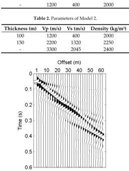
Table 2. Parameters of Model 2.
184
Thickness (m) Vp (m/s) Vs (m/s) Density (kg/m3)
100 1200 400 2000
150 2200 1320 2250
- 3300 2045 2400
185
Figure 1. Synthetic seismic data (mainly surface waves) of Model 1.
186
187
189
(a) (b)
190
Figure 3. Curves of the reconstruction errors of (a) surface waves and (b) reflections against the
191
threshold amplitude.
192
3. Examples
193
3.1. Synthetic examples
194
3.1.1. Distortion of surface-wave dispersive energy caused by reflections
195
Two layered earth models (Model 3 and Model 4) are given in Table 3 and 4 to display the
196
distortion of surface-wave dispersive energy caused by reflections. The layers of Model 3 are the first
197
two layers of Model 4. A synthetic X-component shot gather (Figure 4a) of the Model 3 is simulated
198
using a staggered-grid finite-difference method with an explosive source located at 3-m depth.
199
Another synthetic X-component shot gather (Figure 5a) of the Model 4 is simulated using the same
200
method and the same forward-simulation parameters. We simulated the records with 51 receivers
201
evenly spaced 2 m in line on the surface and the nearest offset of 40 m. As shown in Figure 4b and
202
5b, the two shot gathers are transformed into the f-v domain by high-resolution LRT.
203
According to the relationship between penetration depths of Rayleigh waves and wavelengths
204
[34], the surface waves of Model 3 and Model 4 can’t penetrate into the depth of 100 m so the
205
dispersion characteristics of pure surface waves in Figure 5a should be similar to that in Figure 4a.
206
The surface waves in Figure 4a are not disturbed by the reflections from the deep reflectors. The
207
dispersive energy shown in Figure 4b is continuous and the three branches of dispersion energy are
208
clearly corresponding to the first, second, third higher modes. But the events of higher-mode surface
209
waves in Figure 5a are discontinuous overlapping with the reflections in two-way time of 0.35 s and
210
0.45 s, and it is difficult to discern which higher mode the dispersive energy in frequencies of 25-33
211
Hz and apparent velocities of 470-530 m/s (energy circled in Figure 5b) corresponds to. A comparison
212
of Figure 4b and Figure 5b demonstrates that reflections may disturb the dispersive energy of surface
213
waves. What causes this phenomenon “mode kissing” is the non-negligible effect of the reflections at
214
the range of frequencies and velocities. The picked dispersion curves based on the amplitude and the
215
continuity of dispersive energy are shown in Figure 5c where the second higher mode of frequencies
216
of 25-27 Hz mistakes for the third higher mode. However, the surface-wave dispersive energy on
Z-217
component seismic data is not severely influenced by the reflections from the deep reflectors
218
according to Hu et al. [20].
219
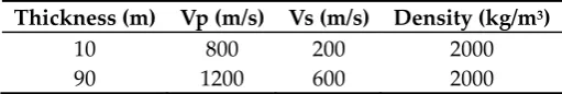
Table 3. Parameters of Model 3.
220
Thickness (m) Vp (m/s) Vs (m/s) Density (kg/m3)
10 800 200 2000
90 1200 600 2000
221
Threshold amplitude
Reco
nstruc
tion errors
Threshold amplitude
Reco
nstruc
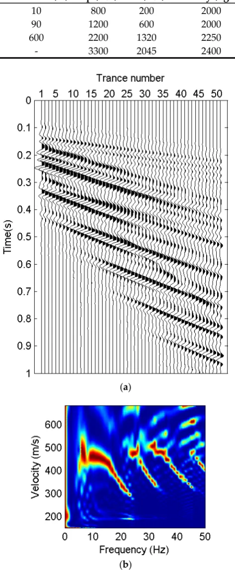
Table 4. Parameters of Model 4.
222
Thickness (m) Vp (m/s) Vs (m/s) Density (kg/m3)
10 800 200 2000
90 1200 600 2000
600 2200 1320 2250
- 3300 2045 2400
223
(a)
(b)
Figure 4. (a) A synthetic X-component shot gather of Model 3 and (b) its image of dispersive energy
224
(a)
(b)
(c)
Figure 5. (a) A synthetic X-component shot gather of Model 4, (b) its image of dispersive energy in
226
the f-v domain and (c) dispersion curves picked from the dispersive energy.
227
Third higher mode
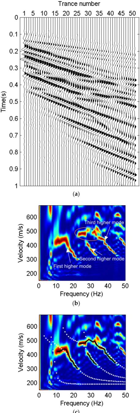
3.1.2. Recovery of the surface-wave dispersive energy
228
The proposed method is applied to the synthetic seismic data shown in Figure 5a to display the
229
result of surface-wave extraction and the improvement of the surface-wave dispersive energy.
230
Compared with the dispersive energy of the original seismic data shown in Figure 5b, the dispersive
231
energy of the surface waves extracted from the data is more continuous in Figure 6. The energy of
25-232
27 Hz and 28-33 Hz is separated to two parts corresponding to the second higher mode and the third
233
higher mode respectively, which means “mode kissing” disappears. Also, the dispersive energy is
234
close to the theoretical dispersion curves, which implies surface waves are effectively extracted using
235
the proposed method.
236
(a)
(b)
Figure 6. (a) Result of surface-wave extraction by the proposed method and (b) its image of dispersive
237
energy in the f-v domain where the white dotted lines represent the theoretical dispersion curves.
238
Furthermore, we compared the proposed method with other methods of surface-wave
239
extraction to test the superiority of the proposed method. High-resolution LRT is applied to the
240
original data and a 2D window is used to select and extract surface waves in the f-v domain. In Figure
7, the result shows surface waves are mainly extracted but “mode kissing” is not changed. The f-k
242
filtering method is also used to extract surface waves. The result of surface-wave extraction consists
243
of residual reflections in Figure 8a and “mode kissing” is reduced in Figure 8b. But there is also a risk
244
of mode misidentification owing to the discontinuous dispersive energy shown in Figure 8b.
245
(a)
(b)
Figure 7. (a) Result of surface-wave separation by a 2D window of the f-v domain and (b) its image
246
(a)
(b)
Figure 8. (a) Result of surface-wave separation by f-k filtering and (b) its image of dispersive energy
248
in the f-v domain.
249
3.2. A field example
250
The X-component field data of 2D3C seismic data shown in Figure 9 were acquired in the
251
Wangjiatun District, Daqing Oilfield, China, with the sample interval of 4 ms, the geophone interval
252
of 25 m and the nearest offset of 400 m. It can be seen that several events of higher-mode surface
253
waves overlap with the reflections. Reflections spread over the f-v domain while surface waves are
254
mainly at the range of low frequencies and low velocities shown in Figure 10. Several branches of
255
dispersive energy at frequencies of ~5 Hz and velocities of 800-1000 m/s circled in Figure 10 are so
256
close to each other resulting in inaccurate phase velocities at those frequencies. By the proposed
257
method, the extracted surface waves are shown in Figure 11a, where most of surface waves are
258
extracted, and the rest of the field data are reflections and other noise except for small amount of
259
surface waves circled in Figure 11b. This is because the morphology of surface waves and reflections
260
may not meet the assumption occasionally in view of the near surface heterogeneity.
261
262
Figure 9. X-component field data of 2D3C seismic data acquired in the Wangjiatun District, Daqing
263
Oilfield, China.
264
265
B
Third mode
Second mode
First mode Fundamental
mode
Trance number
Time (
ms)
Fourth mode
266
267
Figure 10. Image of dispersive energy of the field data in the f-v domain
268
(a) Surface waves
Fourth mode
Third mode
Second mode
Fundamental mode First mode
Trance number
A
B
Time (
(b)
Figure 11. (a) Extracted surface waves by the proposed method and (b) the rest of the field data.
269
To display the effectiveness of surface-wave extraction further, the details of waveform are
270
compared in Figure 12 where the original field data (Figure 9) and the result of surface-wave
271
extraction (Figure 11a) in section A and section B are zoomed. For section A, the original data are
272
dominated by reflections while the surface waves can be easily identified in the result of
surface-273
wave extraction. For section B, surface waves are more clearly and more continuous after
surface-274
wave extraction. The image of dispersive energy of the extracted surface waves using the proposed
275
method is shown in Figure 13a. After surface-wave extraction, the dispersive energy of different
276
modes is separated and the ambiguity of the phase velocities in Figure 10 is eliminated.As shown in
277
Figure 13b, we can easily pick dispersion curves from Figure 13a
.
For comparison, the dispersive278
energy of surface waves separated by the f-k filtering method is displayed in Figure 14, where it is
279
difficult to identify the modes of circled energy
.
The results of the synthetic example and the field280
example demonstrate that surface-wave extraction by the proposed method attenuates the distortion
281
of the surface-wave dispersive energy caused by reflections, which contributes to extracting accurate
282
dispersion curves.
283
284
(a) (b) Trance number
17 19 21 23
Trance number
17 19 21 23
Time (
ms)
Time (s)
(c) (d)
Figure 12. Details of waveform of (a) section A in Figure 9, (b) section A in Figure 11a, (c) section B in
285
Figure 9 and (d) section B and Figure 11a.
286
(a)
(b)
Figure 13. (a)Image of dispersive energy of the extracted surface waves using the proposed method
287
and (b) dispersion curves picked from Figure 13a.
288
289
4. Discussion
291
The advantage of the method over other methods of surface-wave extraction is clear for
X-292
component seismic data while it is not obvious for Z component. The surface-wave dispersive energy
293
on Z component is not severely influenced by the reflections because surface waves and reflections
294
on Z component are clearly in different locations of f-v domain for Z-component seismic data (Hu et
295
al., 2016) where fundamental-mode surface waves are dominated.
296
The main limitation of the method is that surface waves and reflections may not be separated
297
thoroughly in field data. The main problem is that the morphology of surface waves and reflections
298
may deviate the assumption in view of the near surface heterogeneity. In addition, the reflections are
299
not represented by high-resolution HRT sparsely for steep-reflection interfaces so that the
surface-300
wave dispersive energy can’t avoid the influence of reflections. Further research will be conducted to
301
solve the problems.
302
5. Conclusion
303
We propose a method to extract surface waves by exploiting the morphological differences
304
between reflections and surface waves on the basis of MCA. The advantage of this method over the
305
previous techniques is that it can extract surface waves in the case where dispersive energy of
higher-306
mode surface waves overlaps with that of reflections in the f-v domain. It may allow one to separate
307
PS-waves and surface waves whose frequencies and velocities are close. Synthetic and field examples
308
demonstrate that: (1) Frequency-domain high-resolution LRT and time-domain high-resolution HRT
309
are significantly different in the sparse representations for surface waves and reflections, which is
310
suitable for wavefield separation; (2) Reflections may disturb the dispersive energy of surface waves,
311
which makes it difficult to extract dispersion curves of surface waves; (3) Surface waves are
312
effectively extracted by the proposed method and the dispersive energy becomes more continuous
313
and less distorted. Also, dispersion curves picked from the dispersive energy are much more accurate
314
in view of the reliable image of surface-wave dispersive energy.
315
Funding: This research is financially supported by the National Natural Science Foundation of China (Grant
316
Nos. 41425017,41504107,41874166).
317
Acknowledgments: The first author appreciates Jianjun Gao and Chunying Yang for their constructive
318
suggestions on Radon transform and its application to dispersion curve extraction.
319
References
320
1. Xia, J.H.; Miller, R.D.; Park, C.B.; Ivanov, J.; Tian, G.; Chen, C. Utilization of High-Frequency Rayleigh
321
Waves in near-Surface Geophysics. Leading Edge2004, 23, 753-759, doi:10.1190/1.1786895.
322
2. Zhang, Z.; Chen, Y.; Li, F. Reconstruction of the S-Wave Velocity Structure of Crust and Mantle from
323
Seismic Surface Wave Dispersion in Sichuan-Yunnan Region. Chinese Journal of Geophysics (in Chinese)
324
2008, 51, 1114-1122, doi:10.3321/j.issn:0001-5733.2008.04.020.
325
3. Yang, C.Y.; Wang, Y.; Lu, J. Application of Rayleigh Waves on Ps-Wave Static Corrections. Journal of
326
Geophysics & Engineering2012, 9, 90-97, doi:10.1088/1742-2132/9/1/011.
327
4. Meng, X.H.; Guo, L.H. Using Velocity Inversion of Seismic Rayleigh Wave to Compute S-Wave Statics
328
of P-Sv Wave. Oil Geophysical Prospecting (in Chinese)2007, 42, 448-453,
doi:10.3321/j.issn:1000-329
7210.2007.04.017.
330
5. Luo, Y.H.; Xia, J.H.; Liu, J.P. Joint Inversion of Fundamental and Higher Mode Rayleigh Waves.
331
Chinese Journal of Geophysics (in Chinese)2008, 51, 242-249, doi:10.3321/j.issn:0001-5733.2008.01.030.
332
6. Xia, J.H.; Miller, R.D.; Park, C.B.; Tian, G. Inversion of High Frequency Surface Waves with
333
Fundamental and Higher Modes. Journal of Applied Geophysics2003, 52, 45-57,
doi:10.1016/s0926-334
9851(02)00239-2.
335
Rayleigh Waves in Microtremors. Chinese Journal of Geophysics (in Chinese)2014, 57, 2631-2643,
337
doi:10.6038/cjg20140822.
338
8. Kimman, W.P.; Campman, X.; Trampert, J. Characteristics of Seismic Noise: Fundamental and Higher
339
Mode Energy Observed in the Northeast of the Netherlands. Bulletin of the Seismological Society of
340
America2012, 102, 1388-1399, doi:10.1785/0120110069.
341
9. Savage, M.K.; Lin, F.C.; Townend, J. Ambient Noise Cross-Correlation Observations of Fundamental
342
and Higher-Mode Rayleigh Wave Propagation Governed by Basement Resonance. Geophysical
343
Research Letters2013, 40, 3556-3561, doi:10.1002/grl.50678.
344
10. Luo, Y.H.; Xia, J.H.; Miller, R.D.; Xu, Y.X.; Liu, J.P.; Liu, Q.S. Rayleigh-Wave Dispersive Energy
345
Imaging Using a High-Resolution Linear Radon Transform. Pure and Applied Geophysics2008, 165,
903-346
922, doi:10.1007/s00024-008-0338-4.
347
11. Xia, J.H.; Xu, Y.X.; Luo, Y.H.; Miller, R.D.; Cakir, R.; Zeng, C. Advantages of Using Multichannel
348
Analysis of Love Waves (Malw) to Estimate near-Surface Shear-Wave Velocity. Surveys in Geophysics
349
2012, 33, 841-860, doi:10.1007/s10712-012-9174-2.
350
12. Zhang, S.X.; Chan, L.S. Possible Effects of Misidentified Mode Number on Rayleigh Wave Inversion.
351
Journal of Applied Geophysics2003, 53, 17-29, doi:10.1016/s0926-9851(03)00014-4.
352
13. Bao, Q.Z.; Gao, J.H.; Chen, W.C. Ridgelet Domain Method of Ground-Roll Suppression. Chinese
353
Journal of Geophysics2007, 50, 1041-1047.
354
14. Fang, Y.R.; Shen, F.M.; Qiu, K.N. The New Method of Rayleigh Wave Signal Purification Based on
355
Emd. Earthquake Engineering & Engineering Dynamics2017, 01, 64-71.
356
15. Li, J.F.; Li, R.H.; Wang, W.D. Study on the Extraction of Effective Wave Using Analytic Signal Method
357
in Multicomponent Rayleigh Wave Exploration. Coal Geology & Exploration1998, 26, 61-64.
358
16. Lu, J.; Yun, W.; Yang, C.Y. Instantaneous Polarization Filtering Focused on Suppression of Surface
359
Waves. Applied Geophysics2010, 7, 88-97, doi:10.1007/s11770-010-0001-6.
360
17. Lu, J.; Wang, Y.; Chen, J.Y. Noise Attenuation Based on Wave Vector Characteristics. Applied Sciences
361
2018, 8, 672, doi:10.3390/app8050672.
362
18. Pan, D.; Hu, M.; Cui, R.; Li, J. Dispersion Analysis of Rayleigh Surface Waves and Application Based
363
on Radon Transform. Chinese Journal of Geophysics (in Chinese)2010, 53, 2760-2766,
364
doi:10.3969/j.issn:0001-5733.2010.11.025.
365
19. Trad, D.; Sacchi, M.D.; Ulrych, T.J. A Hybrid Linear-Hyperbolic Radon Transform. Journal of Seismic
366
Exploration2001, 9, 303-318.
367
20. Hu, Y.; Wang, L.M.; Cheng, F.; Luo, Y.H.; Shen, C.; Mi, B.B. Ground-Roll Noise Extraction and
368
Suppression Using High-Resolution Linear Radon Transform. Journal of Applied Geophysics2016, 128,
369
8-17, doi:10.1016/j.jappgeo.2016.03.007.
370
21. Sacchi, M.D.; Ulrych, T.J. High-Resolution Velocity Gather and Offset Space Reconstruction.
371
Geophysics1995, 60, 1169-1177, doi:10.1190/1.1443845.
372
22. Trad, D.; Ulrych, T.J.; Sacchi, M.D. Latest Views of the Sparse Radon Transform. Geophysics2003, 68,
373
386--399, doi:10.1190/1.1543224.
374
23. Starck, J.L.; Elad, M.; Donoho, D.L. Redundant Multiscale Transforms and Their Application for
375
Morphological Component Separation. Advances in Imaging & Electron Physics2004, 132, 287-348,
376
doi:10.1016/s1076-5670(04)32006-9.
377
24. Starck, J.L.; Elad, M.; Donoho, D.L. Image Decomposition Via the Combination of Sparse
378
1582, doi:10.1109/tip.2005.852206.
380
25. Chen, W.C.; Wang, W.; Gao, J.H.; Jiang, C.F.; Lei, J.L. Sparsity Optimized Separation of Ground-Roll
381
Noise Based on Morphological Diversity of Seismic Waveform Components. Chinese Journal of
382
Geophysics (in Chinese)2013, 56, 2771-2782, doi:10.6038/cjg20130825.
383
26. Luo, Y.H.; Xia, J.H.; Miller, R.D.; Xu, Y.X.; Liu, J.P.; Liu, Q.S. Rayleigh-Wave Mode Separation by
384
High-Resolution Linear Radon Transform. Geophysical Journal International2009, 179, 254–264,
385
doi:10.1111/j.1365-246x.2009.04277.x
386
27. Jiang, X.X.; Zheng, F.; Jia, H.Q.; Lin, J.; Yang, H.Y. Time-Domain Hyperbolic Radon Transform for
387
Separation of P-P and P-Sv Wavefields. Studia Geophysica Et Geodaetica2016, 60, 91-111,
388
doi:10.1007/s11200-015-0735-y.
389
28. Scales, J.A.; Gerztenkorn, A.; Treitel, S. Fast Ip Solution of Large, Sparse, Linear Systems: Application
390
to Seismic Travel Time Tomography. Journal of Computational Physics1988, 75, 314-333,
391
doi:10.1016/0021-9991(88)90115-5.
392
29. Turner, G. Aliasing in the Tau-P Transform and the Removal of Spatially Aliased Coherent Noise.
393
Geophysics1990, 55, 1496-1503, doi:10.1190/1.1442797
394
30. Ibrahim, A.; Sacchi, M.D. Simultaneous Source Separation Using a Robust Radon Transform.
395
Geophysics2014, 79, V1-V11, doi:10.1190/geo2013-0168.1.
396
31. Trad, D.; Ulrych, T.J.; Sacchi, M.D. Accurate Interpolation with High-Resolution Time-Variant Radon
397
Transforms. Geophysics2002, 67, 25-26, doi:10.1190/1.1468626.
398
32. Sabbione, J.I.; Sacchi, M.D. Restricted Model Domain Time Radon Transforms. Geophysics2016, 81,
399
A17-A21, doi:10.1190/geo2016-0270.1.
400
33. Sabbione, J.I.; Velis, D.R.; Sacchi, M.D. Microseismic Data Denoising via an Apex-Shifted Hyperbolic
401
Radon Transform. In Proceeding of SEG Technical Program Expanded Abstracts, Houston, USA,
402
2013; pp. 2155-2161, doi:10.1190/segam2013-1414.1.
403
34. Chen, X.; Sun, J.Z. An Improved Equivalent Homogenous Half-Space Method and Reverse Fitting
404
Analysis of Rayleigh Wave Dispersion Curves. Chinese Journal of Geophysics (in Chinese)2006, 49, 489–