Reproducing and Regularizing the SCRN Model

1705

Reproducing and Regularizing the SCRN Model

Olzhas Kabdolov, Zhenisbek Assylbekov, Rustem Takhanov

School of Science and Technology, Nazarbayev University

{olzhas.kabdolov, zhassylbekov, rustem.takhanov}@nu.edu.kz

Abstract

We reproduce the Structurally Constrained Recurrent Network (SCRN) model, and then regular-ize it using the existing widespread techniques, such as naïve dropout, variational dropout, and weight tying. We show that when regularized and optimized appropriately the SCRN model can achieve performance comparable with the ubiquitous LSTM model in language modeling task on English data, while outperforming it on non-English data.

Title and Abstract in Russian

Воспроизведение и регуляризация SCRN модели

Мы воспроизводим структурно ограниченную рекуррентную сеть (SCRN), а затем добавляем регуляризацию, используя существующие широко распространенные методы, такие как исключение (дропаут), вариационное исключение и связка параметров. Мы показываем, что при правильной регуляризации и оптимизации показатели SCRN сопоставимы с показателями вездесущей LSTM в задаче языкового моделирования на английских текстах, а также превосходят их на неанглийских данных.

1 Introduction

Recurrent neural networks (RNN) have demonstrated tremendous success in sequence modeling in gen-eral and in language modeling in particular. The most basic RNN (Elman, 1990) suffers from the problem of vanishing and exploding gradients (Bengio et al., 1994) and is hard to train efficiently. One of the most widespread and efficient alternatives to the basic RNN is the Long-Short Term Memory (LSTM) model (Hochreiter and Schmidhuber, 1997), which effectively addresses the problem of vanishing gradients. However, LSTM is a fairly complex model with excessive number of parameters and its inner function-ality is not obvious. This complexity has motivated some of the researchers to find more apparent and less complex alternatives. One of such alternative models is a Structurally Constrained Recurrent Net-work (SCRN) proposed by Mikolov et al. (2015). They encouraged some of the hidden units to change their state slowly by making part of the recurrent weight matrix close to identity, thus forming a kind of longer term memory and showed that their SCRN model can outperform the simple RNN and achieve the performance comparable with the LSTM under no regularization and small parameter budget. It is natural to try to regularize the SCRN model under larger budgets: Will it approach the performance of LSTM?Our experiments show that (1) under naïve dropout the SCRN demonstrates performance close to that of the LSTM, but (2) under variational dropout and weight tying the LSTM demonstrates better performance.

2 Related Work

There has been several attempts on simplifying the ubiquitous LSTM model while not losing in perfor-mance. E.g., Ororbia II et al. (2017) introduced Delta-RNN architecture for which SCRN serves as a

predecessor. They showed that, when regularized using naïve dropout (Zaremba et al., 2014), Delta-RNN performs comparably to LSTM and GRU (Chung et al., 2014). However, they did not compare to regularized SCRN, and they did not consider more recent regularization techniques, such as variational dropout (Gal and Ghahramani, 2016) and weight tying (Inan et al., 2017; Press and Wolf, 2017).

Lei and Zhang (2017) proposed the Simple Recurrent Unit (SRU) architecture, a recurrent unit that simplifies the computation and exposes more parallelism. In SRU, the majority of computation for each step is independent of the recurrence and can be easily parallelized. SRU is as fast as a convolutional layer and 5–10x faster than an optimized LSTM implementation. The authors study SRUs on a wide range of applications, including classification, question answering, language modeling, translation and speech recognition. However, one important thing which needs to be mentioned is that this model also exploits the idea of highway connections (Zilly et al., 2017) letting the input directly flow into the hidden state. The use of highway connections could be the main reason why the model achieves high performance, especially in a multi-stacked setting.

Lee et al. (2017) introduced Recurrent Additive Network (RAN), a new gated RNN which is distin-guished by the use of purely additive latent state updates. At every time step, the new state is computed as a gated component-wise sum of the input and the previous state, without any of the non-linearities commonly used in RNN transition dynamics. The authors show that the model performs on par with the LSTM, and claim that it has significantly less parameters. However, in their language modeling ex-periments the authors specify only the number of parameters in the recurrent units, and do not take into account parameters of the embedding and softmax layers, which actually make up most of the language model parameters.

3 Baseline SCRN Model

LetW be a finite vocabulary of words. We assume that words have already been converted into in-dices. Based on one-hot word embeddings x1:k = x1, . . . ,xk for a sequence of wordsw1:k, the

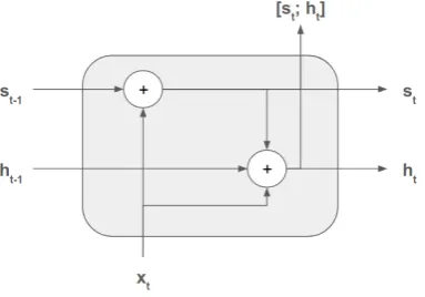
base-line SCRN model (Mikolov et al., 2015) produces two sequences of states,s1:kandh1:k, according to1

Figure 1: SCRN cell.

st = (1−α)xtB+αst₋1, (1) ht=σ(xtA+stP+ht−1R), (2)

whereB ∈R|W|×ds_,A ∈R|W|×dh_,P ∈ Rds×dh_,R∈ Rdh×dh_,d

sanddh are dimensions ofst andht,σ(·)is

the logistic sigmoid function. Mikolov et al. (2015) refer tost as a slowly changingcontext state, and tohtas a quickly changinghidden state. The last couple of states

(sk,hk)is assumed to contain information on the whole sequencew1:kand is further used for predicting the next

wordwk+1 of a sequence according to the probability distribution

Pr(wk+1|w1:k) =softmax(skU+hkV), (3)

whereU ∈ Rds×|W| _andV ∈ Rdh×|W|_{are output embedding matrices. For the sake of simplicity we} omit bias terms in (2) and (3).

Training the model involves minimizing the negative log-likelihood over the corpusw1:K:

−∑K

k=1log Pr(wk|w1:k−1)−→minΘ, (4)

which is usually done by truncated backpropagation through time (Werbos, 1990). HereΘdenotes the set of all model parameters.

1_{Vectors are assumed to be row vectors, which are right multiplied by matrices (xW+b). This choice is somewhat}

Notice that SCRN is a slight modification of the vanilla RNN model (Elman, 1990), and its simplicity (see Fig. 1) is in stark contrast with the complexity of the widespread LSTM model.

Dense embeddings:The original model spends

2· |W| ·(ds+dh) (5)

parameters to embed words into dense vectors at input and at output. We believe that it is more beneficial to first embed words wt into dense vectors wt = xtE ∈ Rdh using only one embedding matrixE ∈

R|W|×dh_{and then usewtinstead ofxtin (1) and (2) with the appropriate change of shapes for matrices:}

B∈Rdh×ds_andA∈Rdh×dh_{. In this case, the model spends}|W|·_(2d

h+ds)parameters on input/output

embeddings, which is ds · |W| parameters less than (5). E.g., on the Penn Tree Bank (PTB) dataset

(Marcus et al., 1993), where|W|= 10,000, the reduction is 1M parameters for the SCRN model with

ds= 100.

4 Stacking and Regularizing the SCRN

4.1 Stacking recurrent cells

It is well known that stacking at least two layers in recurrent neural networks is beneficial, but between two and three layers the results are mixed (Karpathy et al., 2016; Laurent and von Brecht, 2017). To make our results comparable to the previous works on LSTM language modeling (Zaremba et al., 2014; Gal and Ghahramani, 2016; Inan et al., 2017), we experiment with two-layered architectures: the output of the first layer (1, 2) is concatenated[st;ht]and is fed as input into the second layer.

In what follows the superscript index in round brackets denotes the layer index,ξ(p) = [ξ1, . . . , ξd]is

a random vector (dropout mask) withξi ∼Bernoulli(1−p),dis the dimensionality of the corresponding

layer, pis a dropout rate, and ⊙is the element-wise (Hadamard) product. One time-step of a stacked SCRN model is fully specified by the following equations:

• Input embedding layer:

wt:=yt(0)=xtE. (6)

• Two SCRN layers: forl= 1,2

st(l)= (1−α)yt(l−1)B(l)+αst−1(l),

ht(l)=σ

(

yt(l−1)A(l)+st(l)P(l)+ht−1(l)R(l)

) ,

yt(l)= [st(l);ht(l)]. (7)

• Softmax prediction:

Pr(wt+1|w1:t) =softmax

(

yt(2)

[

U V

])

. (8)

In the equations above, the matrices UandV are concatenated along the first dimension to produce a

(ds+dh)× |W|matrix.

4.2 Naïve dropout

Due to high complexity of deep neural networks the regularization techniques are crucial for good gen-eralization performance. Zaremba et al. (2014) proposed one of the ways how dropout (Srivastava et al., 2014) can be used to regularize recurrent neural networks. They apply dropout only to non-recurrent connections, while keeping the recurrent connections without change. This method, usually referred to asnaïve dropout, improves the baseline results of the LSTM model without any other modifications. Application of the same dropout technique to the SCRN model (6, 7, 8) is specified by

ŷt(0)=yt(0)⊙ξt(0)(pi),

ŷt(l) =yt(l)⊙ξt(l)(po), l= 1,2

4.3 Variational dropout

The approach of Zaremba et al. (2014) have led many to believe that dropout cannot be extended to re-current connections, leaving them with no regularization. However, Gal and Ghahramani (2016) showed that it is possible to derive a variant of dropout which successfully regularizes recurrent connections. In their dropout variant, which is usually referred to asvariational dropout, they repeat the same dropout mask at each time step for inputs, recurrent layers, and outputs:

ỹt(0) =yt(0)⊙ξ(0)(pi),

ħt(l)=ht(l)⊙ξ(l)(ph), l= 1,2 (9)

ỹt(l) =yt(l)⊙ξ(l)(po), l= 1,2

whereph is a recurrent dropout rate. This is in contrast to the naïve dropout where different masks are

sampled at each time step for the inputs and outputs alone and no dropout is used with the recurrent connections. Notice that we do not regularize the context statestin horizontal (recurrent) direction.

4.4 Tying word embeddings

Tying input and output word embeddings in word-level RNNLM is a regularization technique, which was introduced earlier (Bengio et al., 2003; Mnih and Hinton, 2007) but has been widely used relatively recently, and there is empirical evidence (Press and Wolf, 2017) as well as theoretical justification (Inan et al., 2017) that such a simple trick improves language modeling quality while decreasing the total number of trainable parameters almost two-fold, since most of the parameters are due to embedding matrices. In case of the SCRN model, reusing input embeddings at output can be done by setting

V=E⊤

in the softmax layer (8).

5 Experimental setup

We use perplexity (PPL) to evaluate the performance of the language models. Perplexity of a model over a sequence[w1, . . . , wK]is given by

PPL=exp (

−1

K

∑K

k=1log Pr(wk|w1:k−1) )

.

Data sets: The baseline model is trained and evaluated on the PTB (Marcus et al., 1993), while all regularized and stacked configurations are trained and evaluated on the PTB and the WikiText-2 (Merity et al., 2017) data sets. For the PTB we utilize the standard training (0-20), validation (21-22), and test (23-24) splits along with pre-processing per Mikolov et al. (2010). WikiText-2 is an alternative to PTB, which is approximately two times as large in size and three times as large in vocabulary.

Baseline Model:To reproduce the results of the baseline (single-layer and non-regularized) SCRN model we use the originalTorchimplementation2released by Mikolov et al. (2015). We have spent fair amount of time and effort to make their script run, as several of its dependencies have not been updated for few years, and are not compatible with the up-to-date versions of the others. To simplify the path for other researchers we release a script3, which installs necessary versions of the dependencies. We use exactly the same set of hyperparameters reported in the original paper (Table 1). We also implement the baseline SCRN model ourselves4usingTensorFlow(Abadi et al., 2016) which, unlikeTorch, uses static computational graphs, and thus has different style of truncated backpropagation through time5(BPTT). Because of this difference, we chose different set of hyperparameters for our implementation (Table 1),

2_{https://github.com/facebookarchive/SCRNNs}

3_{https://github.com/zh3nis/scrn/blob/master/scrnn_deps.sh} 4

Our implementation is available athttps://github.com/zh3nis/scrn

Hyperparameter Mikolov et al. (2015) Our implementation

αin (1) 0.95 0.95

batch size 32 20

initial LR 0.05 0.8

LR decay 1/1.5 0.5

LR decayed if valid PPL doesn’t improve valid PPL doesn’t improve

BPTT steps 50 35

BPTT frequency 5 35

gradients renormalized norms clipped at 5

weights initialized over [−0.05,0.05] [−0.3,0.3]([−0.2,0.2])

Table 1: Hyperparameters of the baseline SCRN model. Abbreviations: LR — learning rate, BPTT — backpropagation through time. Values in brackets correspond to the(dh, ds) = (300,40)configuration

when they differ from others.

and this choice is motivated by the previous work on word-level language modeling (Zaremba et al., 2014), which has an open-source implementation inTensorFlow6_.

Stacked and Regularized Models: In the previous works on regularizing the LSTM, small-sized models usually haddh = 200and medium-sized models haddh = 650. The inner simplicity of the SCRN cell

allows us slighlty larger hidden sizes: we usedh = 240for small models anddh = 750for medium

models. Context state sizesds are chosen to be 40 (small) and 120 (medium), so that total number of

parameters does not exceed the budget, which is 5M parameters for small models, and 20M parame-ters for medium models. We find empirically, that a good ratio between context size and hidden size in the SCRN model is around1/6. We optimize hyperparameters separately under naïve dropout and under variational dropout. Some of the hyperparameters are tuned using random search according to the marginal distributions:

• pi ∼U[0.01,0.6],

• ph ∼U[0.01,0.6],

• po∼U[0.01,0.6],

• initial learning rate∼U[0.5,0.99], • learning rate decay∼U[0.5,0.89], • initialization scale∼U[0.05,0.3].

whereU[a, b]means continuous uniform distribution over the interval[a, b], and initialization scale is a numberrsuch that all model weights are initialized uniformly over[−r, r]. Other hyperparameters are tuned manually through trial-and-error. When performing random search we first choose ranges men-tioned above. After 100 runs the initial ranges are shrinked to the neighborhoods of the values that give best performances, and the random search is performed again. We repeat this procedure until hyperpa-rameters converge to their (sub)optimal values. To prevent exploding gradients we clip the norm of the gradients (normalized by minibatch size) at 5. For training (4) we use stochastic gradient descent.

6 Results

Baseline: To assure that our implementation of the baseline SCRN is adequate, we evaluate it against the original SCRN code by Mikolov et al. (2015) (Table 2). As one can see, the original SCRN code does notfully reproduce the results reported in the original paper. Their hyperparameters (Table 1) work well for the case when(ds, dh) ∈ {(40,10),(90,10)}, but are not optimal for the other two configurations.

Our implementation together with our set of hyperparameters (Table 1) brings the validation and test perplexities ofallthe configurations closer to those reported in the paper.

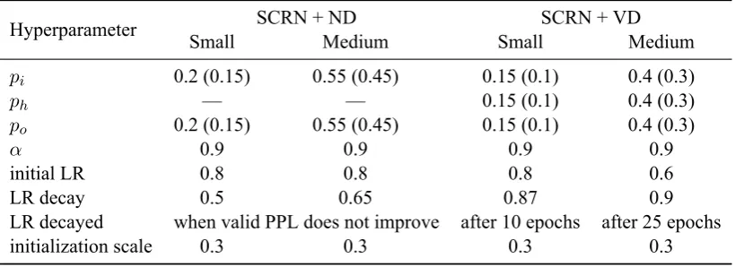
Stacked and Regularized Models: Tuning the stack of two SCRNs results in hyperparameters in Table 3. The results of evaluating these models against regularized and stacked LSTMs on PTB and WikiText-2 are provided in Table 4. Regularization does benefit the simple and intuitive SCRN model, which

Hidden Context Mikolov et al. (2015) Our implementation size size Valid PPL Test PPL Valid PPL Test PPL

40 10 133.6 (133) 127.5 (127) 134.5 128.0

90 10 125.4 (124) 120.3 (119) 124.9 118.6

100 40 127.6 (120) 122.9 (115) 124.9 118.7

300 40 130.1 (120) 124.4 (115) 127.2 120.6

Table 2: Reproducing the baseline model on PTB data. For the original implementation (columns 3 and 4), values outside brackets were obtained when running the script from https://github.com/ facebookarchive/SCRNNs, and values in brackets were reported in the paper of Mikolov et al. (2015).

Hyperparameter SCRN + ND SCRN + VD

Small Medium Small Medium

pi 0.2 (0.15) 0.55 (0.45) 0.15 (0.1) 0.4 (0.3)

ph — — 0.15 (0.1) 0.4 (0.3)

po 0.2 (0.15) 0.55 (0.45) 0.15 (0.1) 0.4 (0.3)

α 0.9 0.9 0.9 0.9

initial LR 0.8 0.8 0.8 0.6

LR decay 0.5 0.65 0.87 0.9

LR decayed when valid PPL does not improve after 10 epochs after 25 epochs

initialization scale 0.3 0.3 0.3 0.3

Table 3: Tuned hyperparameters: ND – naïve dropout, VD – variational dropout. Values in brackets correspond to the WikiText-2 in cases when they differ from those used for the PTB.

demonstrates performance comparable to the sophisticated LSTM model under the naïve dropout, but lags behind the LSTM under the variational dropout regularization. This shows that at some point less complex models become less competitive, even when regularized and optimized appropriately. It is important to mention that no architectural modifications were applied to the original SCRN model except stacking.

Our feeling is that a little over-parameterization of the recurrent connections modelisneeded for the recent regularization techniques to work well. For example, consider the variational dropout of the re-current connections (9) in the SCRN: dropping the coordinatesi1,. . .,ilin the rowht is equivalent to

zeroing out the rowsi1,. . .,ilin the matricesA,P,R. Now consider one layer of the LSTM model:

ft=σ(xtWf+ht−1Uf+bf)

it=σ(xtWi+ht₋1Ui+bi)

ot =σ(xtWo+ht₋1Uo+bo)

ct =ft⊙ct₋1+it⊙tanh(xtWc+ht−1Uc+bc) ht =ot⊙tanh(ct)

When one drops the coordinatesi1,. . .,ilofhtin LSTM, this can be understood as zeroing out the rows

i1,. . .,ilin the matricesWf, Wi,Wo, Uf,Ui,Uo, i.e. around 3 times more parameters are zeroed out

given the same hidden state sizedh. In other words, the number of recurrent weights is 3 times larger in

LSTM than in SCRN. We believe this is one of the reasons why the variational dropout works worse in SCRN. Roughly speaking, there is nothing much to regularize in the horizontal (recurrent) direction in SCRN, as most parameters are in the embedding and softmax layers.

6.1 Ablation analysis

Word-level model PTB WikiText-2 Small Medium Small Medium

LSTM + ND (Jozefowicz et al., 2015) — 79.8 — —

LSTM + ND (Kim et al., 2016) 97.6 85.4 116.8† —

LSTM + ND (Zaremba et al., 2014) — 82.7 — 96.2‡

SCRN + ND 95.8 85.6 115.0 100.8

SCRN + ND + WT 94.1 86.1 112.0 98.5

LSTM + VD (Gal and Ghahramani, 2016) — 78.6 — —

LSTM + VD (Inan et al., 2017) 87.3 77.7 105.9 95.3

LSTM + VD + WT (Inan et al., 2017) 85.1 73.9 100.5 87.7

SCRN + VD 97.2 90.7 120.1 107.6

SCRN + VD + WT 96.8 90.7 112.2 106.0

Table 4: Evaluation of the SCRN against LSTM under different regularization techniques: ND – naïve dropout, VD – variational dropout, WT – weight tying. †We reproduced the LSTM-Word-Small model from Kim et al. (2016) on PTB and then evaluated it on WikiText-2. ‡We ran the open-source imple-mentation from https://github.com/tensorflow/models/tree/master/tutorials/rnn/ptb

at medium config on WikiText-2 data.

parts of the model are more important. The model and dropout variations are listed below.

Removing regularization:To understand how much improvement is gained by the use of regularization we completely remove dropout and weight tying:

pi=po= 0, V̸=E⊤

Removing dropout of the context state: According to (1), context state st changes linearly and thus should not suffer from over-fitting. Thus it seems reasonable to try to not regularize it and apply dropout only to the hidden states, i.e. replacing the equation (7) by

yt(l)= [st(l);ht(l)⊙ξt(l)(po)], l= 1,2.

Removing the context state from the softmax layer:As in the case of the SCRN, the inner state of the LSTM model also consists of two vectorsct andht, and usually the statectis not used at softmax. We

do the same for the context statestin our model, i.e. the equation (8) is replaced by

Pr(wt+1|w1:t) =softmax(ht(2)V).

The meaningfulness of removing the context state from the softmax is that, in our opinion, it plays the role of a long-term memory and thus should not be crucial for predicting the next word of a sequence. Moreover, such removal reduces the model size by at leastds· |W|parameters, which can be significant

(see Section 3).

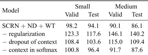
The results of the ablation analysis are provided in Table 5. As we can see, without regularization our SCRN + ND + WT model fails to generalize well on validation and test sets. Regularizing only the hidden state (and keeping the context state untouched) is less harmful but still degrades the performance of the model. Finally, not using the context state in the output only slightly worsens the performance but at the same time leads to a significant reduction in model size.

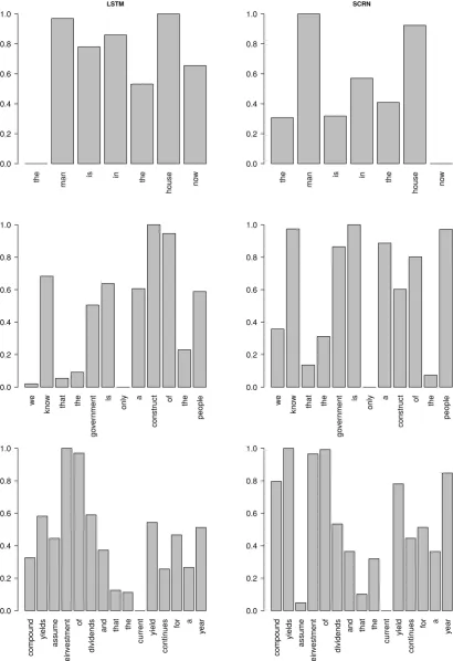
6.2 Hidden state changes

the _man is in the house no w LSTM 0.0 0.2 0.4 0.6 0.8 1.0

the _man is in the

house no w SCRN 0.0 0.2 0.4 0.6 0.8 1.0 w e kno w that the go vernment is onl y a cons

truct of the

people 0.0 0.2 0.4 0.6 0.8 1.0 w e kno w that the go vernment is onl y a cons

truct of the

people 0.0 0.2 0.4 0.6 0.8 1.0 com pound yields assume rein ves tment of dividends

and that the

curr ent yield continues for a year 0.0 0.2 0.4 0.6 0.8 1.0 com pound yields assume rein ves tment of dividends

and that the

curr ent yield continues for a year 0.0 0.2 0.4 0.6 0.8 1.0

Model Small Medium Valid Test Valid Test

SCRN+ND+WT 98.2 94.1 90.1 86.1

−regularization 123.3 117.6 146.1 140.2

−dropout of context 108.4 103.6 115.0 109.4

−context in softmax 100.8 96.4 91.7 87.6

Table 5: Model ablations for the small and medium SCRN + ND + WT models on PTB set.

7 Sobolev Regularization

Together with dropout and weight tying techniques we conducted some experiments with a Sobolev-type regularization. By the Sobolev-Sobolev-type regularization we understand penalization of large gradients of certain parts of neural architecture treated as functions. The idea of penalizing norm of gradients can be traced back to the works on double backpropagation (Drucker and Le Cun, 1992). Zilly et al. (2017) demonstrated that an important property of the hidden vector’s dynamics is its stability, which they decribe in terms of an upper bound on norm of Jacobian matrix ∂ht

∂ht−1. Exploiting the latter intuition

we suggest the following regularization term:

LSobolev=β K

∑

t=1 ∂ht

∂ht₋1

2

F

, (10)

where∥A∥F =

√

Tr(A⊤A)is the Frobenius norm of a matrixA. Note that we do not specify the layer, since our regularization can be applied to all layers, as well as to certain layers only. The strength of such penalty is controlled by the hyperparameterβ.

Overall, our experimental results are consistent with conclusions to which we came for variational dropout, with a perplexity gain even smaller than in the latter case. A typical gain from the Sobolev-type regularization was up to 1 perplexity point when it was applied on top of naïve or variational dropout, and up to 7 perplexity points when it was the only regularization used. Based on those results, the conclusion from Section 6 can be reinforced: probably, the main weakness of SCRN model, in comparison with pop-ular RNNs for which the regpop-ularization of recurrent connections is effective, is under-parameterization of those connections. The latter “does not give a space” for such regularization techniques. For complete-ness of narrative, let us give some details of implementing the Sobolev term inTensorFlow.

Since htis a row, then _∂∂_hh_t−t₁ is understood as

[

∂hjt

∂hi t−1

]

(i.e. transposed Jacobian ∂ht⊤

∂ht−1⊤). According

to (2), we haveht =σ(xtA+stP+ht−1R). After an application of the matrix chain rule, we obtain:

∂ht

∂ht₋1

=R·diag(σ′(at+ht−1R)),

whereat=xtA+stPand diag(v)is a diagonal matrix with its diagonal consisting of the components of

a vectorv. Further, we have:

∂ht

∂ht₋1

2 F =Tr ( ∂ht

∂ht₋1 ⊤ _∂ht

∂ht₋1

)

=Tr

(

diag(σ′(at+ht₋1R))·R⊤R·diag(σ′(at+ht₋1R))

) .

Using the fact that trace is invariant w.r.t. to the transformA → S−1AS, we can setS =diag(σ′(at+ ht₋1R))and obtain the final formula:

∂ht

∂ht−1 2

F

where forR = [r1, . . . ,rdh],v(R)is defined as the column

[

∥r1∥2, . . . ,∥rdh∥

2]⊤_{. Finally, the Sobolev}

term (10) can be given as

LSobolev=β

[ _K ∑

t=1

(σ′)2(at+ht−1R)

]

v(R),

which is a form of a loss function that is suitable for an efficient implementation inTensorFlow(we also used the standard trick thatσ′(x) =σ(x)(1−σ(x))).

8 Performance on non-English data

It is interesting to see the performance of SCRN on texts written in non-English languages. For this purpose we conduct evaluation of the medium-sized versions of LSTM + VD + WT against SCRN + ND + WT on non-English data which comes from the 2013 ACL Workshop on Machine translation7with pre-processing per Botha and Blunsom (2014). Hyperparameters tuned on Wikitext-2 (Table 3) were used for all languages and we did not perform any language-specific tuning. Corpora statistics and the results of evaluation are provided in Table 6. Surprisingly, the SCRN model performs very well (compared to

French Spanish German Czech Russian

Number of tokens 1M 1M 1M 1M 1M

Vocabulary size 25K 27K 37K 46K 62K

LSTM + ND (Kim et al., 2016) 222 200 286 493 357

LSTM + VD + WT 205 193 277 488 351

SCRN + ND + WT 199 179 258 420 306

Table 6: Evaluation of medium-sized models on non-English data.

LSTM) when it comes to modeling morphologically rich languages. Also, it is noteworthy that the higher the type-token ratio, the bigger the advantage of SCRN over LSTM. Our hypothesis for this phenomenon is as follows: in a morphologically rich language one needs less previous words (context) on average to predict the next word than in English, e.g.

German: Pr(lag|Der, einschlagspunkt)

English: Pr(was|The, location, of, the, impact)

The parameterαin the SCRN model (1) controls how much of the previous context is stored in the slowly changing state st. Under the mentioned hypothesis, for the morphologically rich language an optimal value ofαshould be lower than for English. To verify this we train the medium-sized SCRN + ND + WT on all datasets for different values ofα, and the results are provided in Table 7. Indeed, as we can see,

α PTB WikiText-2 FR ES DE CS RU

0.85 88.0 101.1 205 184 264 439 313

0.88 87.5 99.5 198 183 262 422 309

0.90 86.1 98.5 199 179 258 420 306

0.95 87.2 97.8 197 179 260 425 307

0.97 86.0 96.5 199 180 261 437 313

0.99 92.4 100.0 213 190 287 479 326

Table 7: Performance of SCRN + ND + WT for different values ofα.

α = 0.9is more beneficial for German, Czech and Russian (TTR>0.03), butα = 0.97is better for English PTB and WikiText-2 (TTR<0.03), whileα= 0.95is optimal for French and Spanish (TTR≈ 0.03). Also, notice thatα = 0.99brings the SCRN’s results closer to the LSTM’s results on non-English data. Therefore, we think LSTM stores too much of the long-term memory via its trainable forget gate, while in SCRN we can directly control this through theα.

9 Conclusion

Being originally implemented inTorch, the SCRN model is fully reproducible inTensorflowdespite the difference in styles of truncated BPTT in these two libraries. Being conceptually much simpler, the SCRN architecture demonstrates performance comparable to the widely used LSTM model in language modeling task under naïve dropout, but it underperforms the LSTM under variational dropout regular-ization on English data. However, on texts written in morphologically rich languages, the SCRN with appropriately chosen hyperparameterαoutperforms the LSTM.

Acknowledgement

We gratefully acknowledge the NVIDIA Corporation for their donation of the Titan X Pascal GPU used for this research. The work of Zhenisbek Assylbekov has been funded by the Committee of Science of the Ministry of Education and Science of the Republic of Kazakhstan, contract # 346/018-2018/33-28, IRN AP05133700. The authors would like to thank anonymous reviewers for their valuable feedback.

References

Martín Abadi, Paul Barham, Jianmin Chen, Zhifeng Chen, Andy Davis, Jeffrey Dean, Matthieu Devin, Sanjay Ghemawat, Geoffrey Irving, Michael Isard, et al. 2016. Tensorflow: a system for large-scale machine learning. InProceedings of the 12th USENIX conference on Operating Systems Design and Implementation, pages 265– 283. USENIX Association.

Yoshua Bengio, Patrice Simard, and Paolo Frasconi. 1994. Learning long-term dependencies with gradient descent is difficult. IEEE transactions on neural networks, 5(2):157–166.

Yoshua Bengio, Réjean Ducharme, Pascal Vincent, and Christian Jauvin. 2003. A neural probabilistic language model. Journal of machine learning research, 3(Feb):1137–1155.

Jan Botha and Phil Blunsom. 2014. Compositional morphology for word representations and language modelling. InInternational Conference on Machine Learning, pages 1899–1907.

Junyoung Chung, Caglar Gulcehre, KyungHyun Cho, and Yoshua Bengio. 2014. Empirical evaluation of gated recurrent neural networks on sequence modeling.arXiv preprint arXiv:1412.3555.

Harris Drucker and Yann Le Cun. 1992. Improving generalization performance using double backpropagation.

IEEE Transactions on Neural Networks, 3(6):991–997.

Jeffrey L Elman. 1990. Finding structure in time.Cognitive science, 14(2):179–211.

Yarin Gal and Zoubin Ghahramani. 2016. A theoretically grounded application of dropout in recurrent neural networks. InAdvances in neural information processing systems, pages 1019–1027.

Sepp Hochreiter and Jürgen Schmidhuber. 1997. Long short-term memory. Neural computation, 9(8):1735–1780.

Hakan Inan, Khashayar Khosravi, and Richard Socher. 2017. Tying word vectors and word classifiers: A loss framework for language modeling. InInternational Conference on Learning Representations.

Rafal Jozefowicz, Wojciech Zaremba, and Ilya Sutskever. 2015. An empirical exploration of recurrent network architectures. InInternational Conference on Machine Learning, pages 2342–2350.

Andrej Karpathy, Justin Johnson, and Li Fei-Fei. 2016. Visualizing and understanding recurrent networks. In

International Conference on Learning Representations (Workshop Track).

Thomas Laurent and James von Brecht. 2017. A recurrent neural network without chaos. InInternational Con-ference on Learning Representations.

Kenton Lee, Omer Levy, and Luke Zettlemoyer. 2017. Recurrent additive networks. arXiv preprint arXiv:1705.07393.

Tao Lei and Yu Zhang. 2017. Training rnns as fast as cnns. arXiv preprint arXiv:1709.02755.

Mitchell P Marcus, Mary Ann Marcinkiewicz, and Beatrice Santorini. 1993. Building a large annotated corpus of english: The penn treebank. Computational linguistics, 19(2):313–330.

Stephen Merity, Caiming Xiong, James Bradbury, and Richard Socher. 2017. Pointer sentinel mixture models. In

International Conference on Learning Representations.

Tomáš Mikolov, Martin Karafiát, Lukáš Burget, Jan Černockỳ, and Sanjeev Khudanpur. 2010. Recurrent neural network based language model. InEleventh Annual Conference of the International Speech Communication Association.

Tomas Mikolov, Armand Joulin, Sumit Chopra, Michael Mathieu, and Marc’Aurelio Ranzato. 2015. Learning longer memory in recurrent neural networks. InInternational Conference on Learning Representations (Work-shop Track).

Andriy Mnih and Geoffrey Hinton. 2007. Three new graphical models for statistical language modelling. In

Proceedings of the 24th international conference on Machine learning, pages 641–648. ACM.

Alexander G Ororbia II, Tomas Mikolov, and David Reitter. 2017. Learning simpler language models with the differential state framework. Neural computation, 29(12):3327–3352.

Ofir Press and Lior Wolf. 2017. Using the output embedding to improve language models. InProceedings of the 15th Conference of the European Chapter of the Association for Computational Linguistics: Volume 2, Short Papers, volume 2, pages 157–163.

Nitish Srivastava, Geoffrey Hinton, Alex Krizhevsky, Ilya Sutskever, and Ruslan Salakhutdinov. 2014. Dropout: A simple way to prevent neural networks from overfitting. The Journal of Machine Learning Research, 15(1):1929–1958.

Paul J Werbos. 1990. Backpropagation through time: what it does and how to do it. Proceedings of the IEEE, 78(10):1550–1560.

Wojciech Zaremba, Ilya Sutskever, and Oriol Vinyals. 2014. Recurrent neural network regularization. arXiv preprint arXiv:1409.2329.