Grounding Gradable Adjectives through Crowdsourcing

Grounding Gradable Adjectives through Crowdsourcing

Rebecca Sharp, Mithun Paul, Ajay Nagesh, Dane Bell, and Mihai Surdeanu

{bsharp, mithunpaul, ajaynagesh, dane, msurdeanu}@email.arizona.edu

Abstract

In order to build technology that has the ability to answer questions relevant to national and global security, e.g., on food insecurity in certain parts of the world, one has to implement machine reading technology that extracts causal mechanisms from texts. Unfortunately, many of these texts describe these interactions using vague, high-level language. One particular example is the use of gradable adjectives, i.e., adjectives that can take a range of magnitudes such assmallorslight. Here we propose a method for estimating specific concrete groundings for a set of such gradable adjectives. We use crowdsourcing to gather human language intuitions about the impact of each adjective, then fit a linear mixed effects model to this data. The resulting model is able to estimate the impact of novel instances of these adjectives found in text. We evaluate our model in terms of its ability to generalize to unseen data and find that it has a predictive

R2of 0.632 in general, and 0.677 on a subset of high-frequency adjectives.

Keywords:grounded semantics, gradable adjectives, crowdsourcing

1.

Introduction

In order to understand the interplay of various entities and events in complex systems such as climate change or crop yields, scientists make use of complex quantitative mod-els (e.g., DSSAT (Jones et al., 2003) or AGMIP (Rosen-zweig et al., 2013)) with qualitative hypotheses (e.g., Parry and Rosenzweig (1993), Zhang el al. (2011), Zhao et al. (2017),inter alia). Typically these models must be hand-generated by domain experts through an expensive process that requires extensive literature review and a large amount of time, resulting in only a small fraction of the available in-formation being processed and incorporated into the mod-els. These models are crucial to predicting the vagaries in such complex systems. A timely and accurate assessment of the factors that affect such systems bears directly on the health of the nation and environment (Elliott et al., 2017; Porwollik et al., 2017). Automated machine reading can help create and validate hypotheses using these models, but there remains a disconnect – often relevant events are writ-ten in high-level language, yet the model requires specific quantities. In particular, when describing events, authors often make use ofgradable adjectives, i.e., adjectives (such as small) that can take a range of magnitudes or degrees (e.g., something can be a little small, very small, extraordi-narily small, etc.)

When used to describe important changes in model pa-rameters, as with this snippet from a scientific publica-tion: “...doubling of the atmospheric carbon dioxide con-centration will lead to only asmall decreasein global crop production.” (Parry and Rosenzweig, 1993), the ability to quantify or ground such adjectives is a critical step for au-tomated machine reading. For example, consider the dif-ference between asmall increase in rainfallversus asevere increase in rainfallwhen attempting to predict the funds needed for disaster relief or the potential impact on the ex-pected yield of a given crop.

Here we propose a method for quickly and concretely grounding a large number of gradable adjectives such that their effect can be calculated for entities or events of inter-est. Specifically, we gather human intuitions about the

ef-fect of a particular gradable adjective on a given distribution (i.e., mean and standard deviation), independent of the item being modified, and then use this data to fit a linear model. Gradable adjectives are often classified in terms of scales, e.g., hot, warm, andcool are all in the temperature scale whilelargeandsmalldescribe magnitude instead. Here we focus on these magnitude adjectives as a use case, though we suggest that the method can be straightforwardly ex-tended to other scales.

The resulting resource we provide1 consists of a linear model for each adjective that takes as input the typical dis-tribution of the item being modified and in turn provides the predicted size of the change. Turning once again to the example above, for a region with a average rainfall of 40 inches/year (±6 in), if we need to ground asmallincrease, the model would return a predicted rainfall of 40.54 inches. This can be compared, for example, to 45.26, which is the model’s prediction for alargeincrease.

Our specific contributions are:

• We provide a method for using human language intu-itions about the semantic meaning of gradable adjec-tives to create a viable model for the adjective seman-tics. We decouple the meaning of the adjective from the noun being modified to get a truer semantic under-standing of the adjective itself, and we show that the model predictions are well correlated with the human judgments.

• Using cross validation, i.e., testing on crowdsourced predictions not seen in training but whose adjectives were seen in training, we show that we can achieve a predictive R2 _{of 0.632 when using all adjectives.} When we use a smaller subset of higher frequency ad-jectives, we can fit a higher precision model that has a predictiveR2of 0.677. One limitation of this model is that it is unable to make predictions on novel, or un-seen, adjectives. We address this with an initial

neu-1

All materials, data, and code used are available at

ral network model based on word embeddings. On unseen adjectives this model has a predictive R2 _of 0.244.

• We release the resulting database of 98 adjectives and their corresponding linear models as a domain-agnostic resource. This resource could potentially facilitate the quantification of extracted entities and events that contain gradable adjectives for use in downstream tasks, such as modeling complex systems and predicting real-world events. To address a variety of future use cases, we break this resource down into several versions: the full version with all adjectives that emphasizes recall, a smaller subset that empha-sizes precision, and a second version of each of these that depends only on the adjective (i.e., for when the typical distribution of the noun being modified is un-known).

2.

Related Work

Gradable adjectives have been experimentally demon-strated to be interpreted in part based on the semantics of the nouns they modify (i.e., asmallmouse versus asmall

building) (Bonini et al., 1999; Alxatib and Pelletier, 2011; Bylinina, 2014). For this reason, we test our adjectives us-ing legal non-words (e.g. mards), for which we provide a typical size distribution, and we include the provided dis-tribution in the linear model. This allows us to model the semantics of the adjective in context, while removing the need to test each adjective along with each possible noun it could modify.

Whitman et al. (2003) propose a model for finding percep-tual groundings for adjectives. That is, they ground their adjectives using audio features and are then able to predict a lexical description of unheard music. This is quite sim-ilar to what we do in spirit, however our groundings are numerical rather than perceptual. Several works have at-tempted to link gradable adjectives with numerical quan-tities that co-occur in the context of the gradable adjective mention (Shivade et al., 2016; Narisawa et al., 2013). How-ever, this dependence on corpus resources to find evidence for gradability requires complex information extraction and suffers greatly from sparsity, especially when attempting to ground adjectives in a new domain. Additionally, it results in a solution that is highly domain-specific (Shivade et al., 2016).

Kim and de Marneffe repurposed neural network language models by using word embeddings to rank gradable adjec-tives (2013). Bakhshandeh and Allen (2015) use bootstrap-ping to discover properties of adjectives, including what they can modify. However, rather than simply ranking ad-jectives or extracting their attributes, here we focus on de-termining a concrete, numerical grounding for each. There have also been recent works that use crowdsourcing to determine gradability of adjectives. For example, Qing and Franke (2014) use crowdsourcing to gather intuitions about the interpretation of gradable adjectives, but they are testing whether or not adjective usage corresponds to opti-mal language use, whereas our resource grounds gradable adjectives. Accordingly, they test only four adjectives us-ing visual cues, while we test 98 adjectives usus-ing numerical

Figure 1: Example prompt given to Amazon Mechanical Turk workers to elicit the impact of gradable adjectives. Workers were given a specific distribution (of an imaginary item) and asked for the increase they perceived from the given adjective. The full set of prompts is included with our release.

cues.

The work by Wilkinson and Tim (2016) is closest to our work. They use crowdsourcing to create ranked lists of gradable adjectives that correspond to a variety of differ-ent scales (e.g., temperature, dimension, speed, and so on). Unlike Wilkinson and Tim, we use only one scale (mag-nitude) and again, we are interested in creating a concrete grounding for adjectives rather than a ranking.

3.

Approach

While humans often use high-level language to describe events, models of the interactions between these events re-quire specific quantitative information. To bridge the gap between gradable adjectives and this quantified representa-tion, we use human language intuitions about an adjective’s impact on a given distribution to fit a linear model. With this model, then, we can predict the impact of the adjective on an entity whose distribution is known.

Specifically our approach operates in two parts: gather-ing the human language intuitions for each adjective usgather-ing crowdsourcing (described in Section 4.) and then fitting a linear mixed effects model to the data (described in Sec-tion 5.). The resulting model allows us to make predicSec-tions about the effects of one of our grounded adjectives on un-seen nouns.

4.

Data

desert it would be a large change. However, since we want a model that can be used in a range of contexts, we de-signed our experiment to decouple the adjective semantics from the noun semantics by using non-words for the items being modified (in the style of a “Wug Test” (Berko, 1958)) and providing MTurk workers (turkers) with a typical dis-tribution of the item in question, as shown in the example prompt in Figure 1. We then ask the turkers to describe the effect of the adjective in question on the group size. This response forms the basis for the dependent variable used in our model building.

We required the turkers to be in the United States and in-formed them that they needed to be native speakers of En-glish. To demonstrate this, they were required to correctly answer a language-based question in order to participate. They were given two attempts (i.e., a second question was shown to them if they did not correctly answer the first). For the task, each turker was asked to provide responses to 16 prompts and was compensated with $0.75, based on the average of 20 seconds per prompt.

5.

Model Building

5.1.

Model Factors

As interpretations of gradable adjectives are context-dependent (Section 2.), in addition to the factor of inter-est (i.e., adjective) we include in our model the shape of the distribution for the item being modified using two con-trol factors: the provided mean (µp) and provided standard deviation (σp). We calculateσp directly from the typical range (e.g., 1470 to 2770 in the example in Figure 1), which we consider to be ±2 standard deviations.2 Thus, for the above example,σp = (2770−1470)/4 = 325. The value for the particular group given to turkers (i.e., 2120) lies in the middle of the range and so we use that directly forµp3. We chose not to add the interactions between these factors and adjective due to the large number of degrees of freedom (recall that adjective has 98 levels) in an effort to reduce the likelihood of overfitting.

In addition to differences based on context, gradable ad-jectives have also been shown to be interpreted differently by different individuals (Raffman, 1994; Raffman, 1996; Shapiro, 2006). To account for this, we elected to fit a linear mixed effects model to our data, as this allows us to include a random intercept for each turker. In effect, this means that while we are fitting a linear model with adjective,σp, andµp as fixed effects, we allow the fitted line to have a different intercept for each turker, thereby accounting for individual biases.4 _{While it is possible in this framework}

2

The interpretation ofmostin terms of standard deviations is ambiguous, and may vary between domains. While we have cho-sen to build our model under the interpretation ofmostas±₂ stan-dard deviations, the resulting model could be calibrated to a spe-cific domain by gathering a small set of adjective instances that are accompanied by a specific value. We leave this to future work.

3

In a pilot study we found that neither the direction of the change (i.e.,increasevs. decrease) nor the non-word used sig-nificantly affected the model, so in this study we did not include these as factors.

4_{Note that while random intercepts allow the model to be more} robust to variance due to individual biases, the model included in

Fixed Effects χ2 p-value

µp:σp χ2(1) = 1.98 p= 0.16 µp χ2(1) = 5.59 p <0.05 σp χ2(97) = 151.46 p <0.001

Table 1: Results of the likelihood ratio tests (LRTs) used to de-termine the significance of the model’s fixed effects. Significance was determined through a likelihood ratio test comparing a model with the predictor to a model without.

to also have random slopes for each adjective, here we re-frained so as to avoid a large increase in model complexity. The dependent variable (i.e., what the model is trying to predict) is the response given by the turkers, normalized by µpandσpinto something very similar to a z-score:

respDev= |response−µp| σp

(1)

In this way, arespDevof 0.5 indicates an increase of 0.5 standard deviations from the mean. Boxplots showing the responses for a subset of the adjectives are shown in Fig-ure 2. The collected values for these adjectives align with human intuitions, and we also see something of a floor ef-fect whereby the responses for the adjectives that indicate a smaller change seem to have much lower variance than the responses for the adjectives that indicate a larger change. For example, Figure 2 highlights that there is a small vari-ance in responses forconservativeandslight, but a the large variance in responses forhugeandmajor.

5.2.

Data Cleaning

We initially gathered 50 data points for each of our 98 ad-jectives. However, responses generated using MTurk can be quite noisy, so to reduce the amount of noise in our data we excluded data based on several criteria. We excluded all responses from turkers we considered to be unreliable because more than 50% of their responses were outliers5_,

20% or more of their responses were identical to µp, or 50% or more of their responses were identical to one of the given range endpoints. We also removed responses that were less than or equal to the mean, as all prompts asked for an amount of increase. We then removed outliers by adjec-tive. Finally, we removed responses from turkers who had 4 or fewer responses remaining (for the purposes of model fitting and evaluation). This left a total of 3309 responses for our 98 adjectives.

5.3.

Model Fitting

Our model fitting was done using thelme4package in R (Bates et al., 2015; R Core Team, 2013). The residuals of the model (i.e., respDev ∼ 1 +adj+σp +µp+σp : µp+ (1|turker)) showed that the data was heteroskedastic. That is, as the predicted values from the model increased, so did the magnitudes of the error residuals. To adjust for this, we log-transformedrespDevto createlogRespDev.

our final resource are averaged across respondents, thus allowing predictions for novel instances.

5

0 2 4 6

slight weak small

conser vativ

e fair

moder ate

adequatesubstantial

major huge

n Standard De

viations (respDe

v)

Magnitude of Perceived Increase by Adjective

Figure 2: The magnitudes of the perceived increase for several ad-jectives. The magnitudes are measured as the absolute difference between the survey response and the given mean divided by the given standard deviation.

After verifying that the resulting residual plot showed ho-moskedasticity (see Figure 3), we usedlogRespDevin all subsequent model-building.

We used likelihood ratio tests (LRTs) to determine the sig-nificance of the fixed effects (i.e., our three factors and their interactions) by first building a parent model that included all factors as well a daughter models that each had a fac-tor removed. We then checked to see if the model with the factor removed was significantly different from its parent model. The resulting significances are shown in Table 1. Asσp:µpwas first determined to not be significant, it was removed and the model without this factor was used as the parent model for testing the significance ofσpandµp, both of which were determined to be significant (see Table 1). The final model is given by:

logRespDev∼1 +adj+σp+µp+ (1|turker) (2)

This fitted model itself is our resource. That is, for each adjective, we have a linear function, fadj(µp, σp)that de-scribes its predicted impact of the quantity in question. For example, the adjectivesmallis represented as:

fsmall(µp, σp) =−1.77 + (1.034e−5)µp−(1.123e−3)σp

The predicted new value implied bysmallcan then be cal-culated from this as:

new= (efsmall(µp,σp)_{×σp) +µp}

6.

Alternative Models

6.1.

Backoff Model

Though the standard deviation was significant, it is not al-ways the case that this will be known. For this situation, we also provide a backoff model that does not includeσp. The dependent variable used in this model is the absolute percent change in the mean (log-transformed):

logP ercChange∼1 +adj+µp+ (1|turker) (3)

Figure 3: Residual plot for the model with all factors included:

logRespDev ∼1 +adj+σp+µp+σp :µp+ (1|turker). The residual plot for the final model (withσp : µpremoved) is omitted for space, but it is nearly identical.

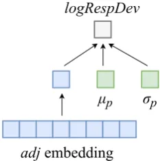
Figure 4: Shallow neural network architecture for predicting the impact of adjectives that were not seen during training using the word embedding of the adjective. As with the linear models, we include the provided mean (µp) and provided standard deviation (σp) as factors and predict the log-transformed response devia-tions (logRespDev).

6.2.

High Frequency (HF) Models

Under the hypothesis that language intuitions will better align for more commonly used words, we additionally re-trained our fitted model and backoff models on a smaller subset of the data that consists of the highest frequency words We sorted the adjectives based on their frequency in the English Gigaword corpus (Graff et al., 2003) and re-tained only the top 30 adjectives. We used this higher fre-quency subset of adjectives to train a regular as well as a backoff model.

6.3.

Grounding Using Neural Networks

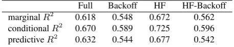
Full Backoff HF HF-Backoff marginalR2 0.618 0.548 0.672 0.562 conditionalR2 0.670 0.589 0.725 0.596 predictiveR2

0.632 0.544 0.677 0.542

Table 2: Estimation from all models of how much of the vari-ance in the data is accounted for by the model’s fixed effects (marginalR2), and both the fixed and random effects (conditional

R2_{). Also, an measure of how well the model predicts new data,}

predictiveR2.

(NN) model which builds upon pre-trained word embed-dings (Mikolov et al., 2013). Intuitively, by using word embeddings trained over a large corpus, we already know some of the underlying semantics of the unseen adjectives. Therefore, to the extent that the embedding of a given adjective captures its implied magnitude, we can learn a mapping from this embedding to the specific, quantitative grounding for the adjective.

In this NN approach, shown in Figure 4, we use a fully-connected hidden layer of size one to compress the adjec-tive’s high-dimensional word embedding to a single value (shown in blue), the activation of which can be directly in-terpreted as the semantic impact of the adjective learned by the model. This value is then concatenated to the pro-vided mean (µp) and provided standard deviation (σp) and passed to an output layer that predicts the the log trans-formed response deviation (logRespDev). In this frame-work we found that the features that uniquely identify the individual respondent from the crowdsourcing experiment were not needed (i.e., they did not greatly improve perfor-mance), and so we removed them to help prevent overfit-ting.

We trained the model using mean squared error as the loss function. The embeddings were initialized with the Glove (Pennington et al., 2014) 300-dimensional pre-trained word embeddings and they were not updated during training (again, to reduce overfitting). A tanh activation was used for the adjective node6 _{and we use the RMSProp}

opti-mizer (Tieleman and Hinton, 2012) with a learning rate of 0.00001 and all other parameters with their default values.

7.

Results

7.1.

Linear Models

For the evaluation of our linear models, we report the marginal and conditional R2 in Table 2. The marginal R2 _{shows the amount of the variance that is explained} by only the fixed effects and the conditional R2 _shows the amount of the variance that is explained by both the fixed and random effects. Both were calculated using ther.squaredGLMMfunction from the MuMIn (Barton, 2016) package, an implementation of the method of Nak-agawa and Schielzeth (2013). As we are primarily inter-ested in using this resource to make predictions about new instances of adjectives, the correlation of the model’s pre-dictions with real data is key. Thus, we also calculate the predictiveR2_{with leave-one-out cross-validation, such that}

6_{We tried using non-linear activations on all the nodes but did} no see an improvement so we omitted them for model simplicity.

Seen Adjs Unseen Adjs Linear Full Model 0.632 –

NN Model 0.540 0.244

Table 3: Comparison of how well the linear mixed effects full model and the neural network (NN) model predict new data (pre-dictiveR2_{). Performance is shown for predictions both on}

adjec-tives that were present in the training data (seen) as well as on adjectives that were not (unseen).

the residual error of each data point (i.e., individual re-sponse) is based on a model trained on all the data ex-cept for that point. Specifically, the predictive R2 _{is the} predicted residual error sum of squares (PRESS) statistic (Allen, 1974) divided by the total sum of squares (SStotal):

R2pred= 1−

(logRespDevi−logRespDev)2 (6)

That is, for each individual response i ∈ D, we sum the residual squared error between the true value, logRespDevi and the value predicted by a model trained on the rest of the data,logRespDev\ i,D\i. We then divide this bySStotaland subtract if from1to get the predictive R2. For our full model, the predictiveR2was 0.632 (also shown in Table 2). This result suggests that the quantities implied by these adjectives can be predicted with reason-able accuracy with simple, linear models trained on crowd-sourced data.

We found that the backoff subset model had a slightly worse fit than the full model. This is expected as it does not con-tain the standard deviation as a factor, which was deter-mined to be significant (Section 5.3.).

The high-frequency (HF) model shows a higherR2_{than the} full model. This confirms that, indeed, language intuitions are more robust for high-frequency adjectives. However, this effect is only seen in the full model when standard de-viation is known.

7.2.

Neural Network Model

We evaluate our neural network (NN) model on both seen and unseen adjectives. The predictiveR2onseenadjectives (i.e., when data points for each adjective are split between training and test folds) can be compared to the performance of the linear models, while the performance onunseen ad-jectives (i.e., when adad-jectives appearing in test folds donot

occur in training folds) indicates utility with novel adjec-tives. Due to time constraints rather than using leave-one-out cross-validation (as with the linear models) we instead use four-fold cross-validation with two folds for training, one for development, and one for testing.

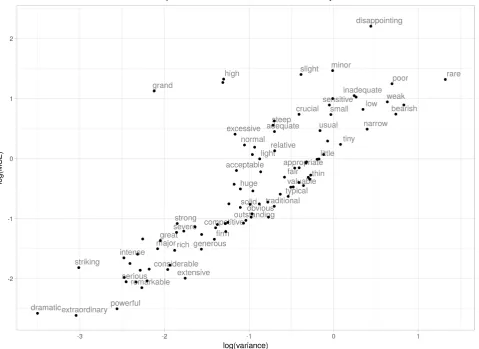
Figure 5: A comparison of the mean squared error (MSE) versus variance for each gradable adjective. The MSE is based on the neural network model predicting on unseen adjectives and the variance is from the original crowdsourced data. Note that the axes are presented in log scale.

On seen adjectives, the NN model performs almost as well as the linear model, and we suspect that the performance difference is primarily due to the larger number of param-eters that need to be learned. Additionally, while the infor-mation about individual turkers was empirically found to not help the NN model, the linear model benefits from its inclusion.

The predictiveR2_{for unseen adjectives is much lower than} for seen adjectives, but recall that the linear model is un-able to make any predictions for these adjectives at all. It is unclear exactly where the performance drop originates, though we hypothesize that it is primarily due to the re-liance on pre-trained word-embeddings. While they allow us to estimate groundings for adjectives that we did not include in training, the estimates are only as good as our capacity to extract the necessary information from the em-bedding. That is, the embeddings were trained to capture distributional similarity, not relative magnitude of impact. Thus, this information, when present, is indirect and very likely noisy.

To better understand the performance of this model, we compared the mean squared error (MSE) of the model on these unseen adjectives with their variance in the origi-nal data from the crowdsourcing experiment. The plot is

shown in Figure 5. Overall, as the variance in the origi-nal data increases, so does the MSE. This suggests that in general adjectives with higher variance are harder to pre-dict. Further, some adjectives had much higher variance (e.g.,rareanddisappointing), suggesting that for some ad-jectives this task is difficult even for humans. Additionally, certain adjectives (such asgrand, high, anddisappointing) had a particularly high MSE. We suspect that this is, again, due to the reliance on the pre-trained emebeddings as many of these words have multiple senses (e.g., disappointing, as withdisappointing increaseversusthe play was disap-pointing), and here the sense we are interested in is not the most frequent. For these words with multiple senses, the embeddings are confounded. To address these issues, ded-icated embeddings that better model the semantics of inter-est could be explored (such as the embeddings proposed by Kim et al. (2016) that are dedicated for modeling adjec-tives). We leave this exploration to future work.

8.

Conclusion

remaining otherwise independent of the item’s identity. The model was trained on approximately 50 values col-lected through crowdsourcing for each of the adjectives in the set. The resulting model has a predictive R2 _of 0.632 on the whole dataset (measured through leave-one-out cross-validation), and a R2 _{of 0.677 on a subset of} high-frequency adjectives. We release all models created for these adjectives, which, we hope, brings us closer to de-veloping technology that answers questions relevant to na-tional and global security from texts containing qualitative statements.

9.

Acknowledgements

This work was funded by the Defense Advanced Research Projects Agency (DARPA) World Modeling Seed program under ARO contract W911NF-17-1-0047.

10.

Bibliographical References

Allen, D. M. (1974). The relationship between variable se-lection and data augmentation and a method for predic-tion.Technometrics, 16(1):125–127.

Alxatib, S. and Pelletier, F. J. (2011). The psychology of vagueness: Borderline cases and contradictions. Mind & Language, 26(3):287–326.

Bakhshandeh, O. and Allen, J. (2015). From adjective glosses to attribute concepts: Learning different aspects that an adjective can describe. InIWCS.

Barton, K. (2016). Mumin: Multi-model inference (r pack-age version 1.15. 6.)[computer software].

Bates, D., M¨achler, M., Bolker, B., and Walker, S. (2015). Fitting linear mixed-effects models using lme4. Journal of Statistical Software, 67(1):1–48.

Berko, J. (1958). The child’s learning of English morphol-ogy. Word, 14(2-3):150–177.

Bonini, N., Osherson, D., Viale, R., and Williamson, T. (1999). On the psychology of vague predicates. Mind & language, 14(4):377–393.

Buhrmester, M., Kwang, T., and Gosling, S. D. (2011). Amazon’s mechanical turk. Perspectives on Psychologi-cal Science, 6(1):3–5.

Bylinina, E. (2014). The Grammar of Standards. Judge-dependence, Purpose-relativity, and Comparison Classes in Degree Constructions. Utrecht University. Elliott, J., Glotter, M., Ruane, A. C., Boote, K. J., Hatfield,

J. L., Jones, J. W., Rosenzweig, C., Smith, L. A., and Foster, I. (2017). Characterizing agricultural impacts of recent large-scale us droughts and changing technology and management. Agricultural Systems.

Graff, D., Kong, J., Chen, K., and Maeda, K. (2003). English gigaword, ldc2003t05. Linguistic Data Consor-tium, Philadelphia.

Jones, J., Hoogenboom, G., Porter, C., Boote, K., Batch-elor, W., Hunt, L., Wilkens, P., Singh, U., Gijsman, A., and Ritchie, J. (2003). The dssat cropping system model. European Journal of Agronomy, 18(3):235–265. Modelling Cropping Systems: Science, Software and Applications.

Kim, J. and de Marneffe, M. (2013). Deriving adjectival scales from continuous space word representations. In

Proceedings of the 2013 Conference on Empirical Meth-ods in Natural Language Processing, EMNLP 2013, 18-21 October 2013, Grand Hyatt Seattle, Seattle, Washing-ton, USA, A meeting of SIGDAT, a Special Interest Group of the ACL, pages 1625–1630.

Kim, J.-K., de Marneffe, M.-C., and Fosler-Lussier, E. (2016). Adjusting word embeddings with semantic in-tensity orders. In Proceedings of the 1st Workshop on Representation Learning for NLP, pages 62–69.

Mikolov, T., Chen, K., Corrado, G., and Dean, J. (2013). Efficient estimation of word representations in vector space. In Proceedings of the International Conference on Learning Representations (ICLR).

Nakagawa, S. and Schielzeth, H. (2013). A general and simple method for obtaining r2 from generalized linear mixed-effects models. Methods in Ecology and Evolu-tion, 4(2):133–142.

Narisawa, K., Watanabe, Y., Mizuno, J., Okazaki, N., and Inui, K. (2013). Is a 204 cm man tall or small? acquisi-tion of numerical common sense from the web. InACL (1), pages 382–391. The Association for Computer Lin-guistics.

Parry, M. and Rosenzweig, C., (1993). The Potential Ef-fects of Climate Change on World Food Supply, pages 1–26. Springer Berlin Heidelberg, Berlin, Heidelberg. Pennington, J., Socher, R., and Manning, C. (2014).

Glove: Global vectors for word representation. In Pro-ceedings of the 2014 conference on empirical methods in natural language processing (EMNLP), pages 1532– 1543.

Porwollik, V., M¨uller, C., Elliott, J., Chryssanthacopoulos, J., Iizumi, T., Ray, D. K., Ruane, A. C., Arneth, A., Balkoviˇc, J., Ciais, P., Deryng, D., Folberth, C., Izaur-ralde, R. C., Jones, C. D., Khabarov, N., Lawrence, P. J., Liu, W., Pugh, T. A., Reddy, A., Sakurai, G., Schmid, E., Wang, X., de Wit, A., and Wu, X. (2017). Spatial and temporal uncertainty of crop yield aggregations. Eu-ropean Journal of Agronomy, 88(Supplement C):10–21. Uncertainty in crop model predictions.

Qing, C. and Franke, M. (2014). Meaning and use of grad-able adjectives: Formal modeling meets empirical data. In Paul Bello, et al., editors,Proceedings of the 36th an-nual meeting of the Cognitive Science Society (CogSci-2014), pages 1204–1209, Austin, TX. Cognitive Science Society.

R Core Team, (2013). R: A Language and Environment for Statistical Computing. R Foundation for Statistical Computing, Vienna, Austria.

Raffman, D. (1994). Vagueness without paradox. The Philosophical Review, 103(1):41–74.

Raffman, D. (1996). Vagueness and context-relativity.

Philosophical Studies, 81(2-3):175–192.

Rosenzweig, C., Jones, J. W., Hatfield, J. L., Ruane, A. C., Boote, K. J., Thorburn, P., Antle, J. M., Nelson, G. C., Porter, C., Janssen, S., et al. (2013). The agricultural model intercomparison and improvement project (ag-mip): protocols and pilot studies. Agricultural and For-est Meteorology, 170:166–182.

Univer-sity Press on Demand.

Shivade, C., de Marneffe, M., Fosler-Lussier, E., and Lai, A. M. (2016). Identification, characterization, and grounding of gradable terms in clinical text. In Pro-ceedings of the 15th Workshop on Biomedical Natural Language Processing, BioNLP@ACL 2016, Berlin, Ger-many, August 12, 2016, pages 17–26.

Sinclair, J. et al. (1987). Collins COBUILD English lan-guage dictionary. Harper Collins Publishers,.

Tieleman, T. and Hinton, G. (2012). Lecture 6.5-rmsprop: Divide the gradient by a running average of its recent magnitude. COURSERA: Neural Networks for Machine Learning.

Whitman, B., Roy, D., and Vercoe, B. (2003). Learning word meanings and descriptive parameter spaces from music. InProceedings of the HLT-NAACL 2003 Work-shop on Learning Word Meaning from Non-linguistic Data - Volume 6, HLT-NAACL-LWM ’04, pages 92–99, Stroudsburg, PA, USA. Association for Computational Linguistics.

Wilkinson, B. and Tim, O. (2016). A gold standard for scalar adjectives. In Nicoletta Calzolari (Conference Chair), et al., editors,Proceedings of the Tenth Interna-tional Conference on Language Resources and Evalua-tion (LREC 2016), Paris, France, may. European Lan-guage Resources Association (ELRA).

Zhang, D. D., Lee, H. F., Wang, C., Li, B., Pei, Q., Zhang, J., and An, Y. (2011). The causality analysis of climate change and large-scale human crisis. Proceedings of the National Academy of Sciences, 108(42):17296–17301. Zhao, C., Liu, B., Piao, S., Wang, X., Lobell, D. B., Huang,