ABSTRACT
DAS, PRIYAM. Bayesian Quantile Regression. (Under the direction of Subhashis Ghoshal.) Quantile regression (QR) is a fundamental approach to quantifying the relation a set of predictors and a response variable especially for skewed response data. In the first chapter, a literature overview has been provided about the existing quantile regression methods. We discuss the key methods from the literature in the field of quantile regression. A simulation study has been also provided to compare the performances of existing popular Bayesian and non-Bayesian methods for univariate case.
In the second chapter, we consider a Bayesian method for simultaneous quantile re-gression on a real variable. A representation of quantile function is given by a convex combination of two monotone increasing functions ξ1 and ξ2 not depending on the pre-diction variables. In a Bayesian approach, a prior is put on quantile functions by putting prior distributions on ξ1 and ξ2. The monotonicity constraint on the curves ξ1 and ξ2 are obtained through a spline basis expansion with coefficients increasing and lying in the unit interval. We put a Dirichlet prior distribution on the spacings of the coefficient vector. We compare our approach with a Bayesian method using Gaussian process prior through an extensive simulation study and some other Bayesian approaches proposed in the literature. Applications to a data on hurricane activities in the Atlantic region and population data of USA are given. This chapter is based on the material in Das and Ghosal (2016c).
In the third chapter, we extend our method of Bayesian quantile regression to the case where the predictor space is multidimensional and the quantile regression depends on the predictors through an unknown linear combination only. This chapter is based on the material in Das and Ghosal (2016c).
is used to put a prior and a Bayesian analysis is performed. We analyze the average daily 1-hour maximum and 8-hour maximum ozone concentration level data of US and California during 2006–2015 using the proposed method. This chapter is based on the material in Das and Ghosal (2016a).
Chapter 1
Introduction
In a regression model, if the distribution of the response variable is highly skewed, tradi-tional mean regression model may fail to describe interesting aspect of the relationship between the prediction and response variables. For instance, if we deal with the income distribution data of a certain state or country, the traditional mean regression will get affected by the outliers, i.e., the income of top 1–2 % people of that region, and hence is of limited use for prediction of income of general people. For example, as mentioned in this link1, more than 35% of the total wealth of the US belongs to top 1% people. So it can be understood that this distribution being heavy-tailed, regular mean regression might not be a good representative of the average per-capita wealth of the US. This situation arises often in business, economics, environmental and many other fields. As an alternative to traditional linear regression, quantile regression (QR) is one of the most popular and useful regression technique.
Frequentist single Quantile Regression methods
Quantile regression (QR) was first proposed in Koenkar and Bassett (1978). Suppose our univariate observations are given by {Yt:t= 1, . . . , T}. So theτ-th quantile (0 < τ <1) of the observations can be found solving the optimization problem given by
min b∈R
X
t∈{t:Yt≥b}
τ(Yt−b) +
X
t∈{t:Yt<b}
(1−τ)(b−Yt)
.
It is noted that putting τ = 12 in the above equation yields the median. But, this more general form to find the quantiles is helpful specially when we are interested in the
behavior of the tail distributions. In case we have the explanatory variables {Xt ∈ Rk :
t= 1, . . . , T, k ∈N}, the τ-th (0< τ <1) linear quantile regression coefficient β ∈Rk is given by
min b∈R
X
t∈{t:Yt≥Xtβ}
τ|Yt−Xtβ|+
X
t∈{t:Yt<Xtβ}
(1−τ)|Yt−Xtβ|
.
Thus the method proposed by Koenkar and Bassett (1978) (KB method) can be used to find the linear regression coefficients for any specified quantile.
Due to computational convenience and other theoretical properties, the method pro-posed by Koenkar and Bassett (1978) remained popular for long time. Later on, several works emerged studying the asymptotic properties and procedures of estimating its stan-dard error along with some extensions and improvements of single quantile regression from the frequentist’s point of view; see Gutenbrunner and Jureckova (1992), Guten-brunner et al. (1993), Koenker and Xiao (2002), Zhou and Portnoy (1996), Koenker and Machado (1999). Geraci and Bottai (2007) proposed the single level quantile regression model with subject specific random intercept term which accounts for within group cor-relation.
Bayesian single Quantile Regression
One of the first attempts for Bayesian quantile regression was proposed in Yu and Moyeed (2001) (YM method). Consider the standard form of the linear model
Yt=µ(Xt) +t
where µ(Xt) is the conditional mean of Yt given the regressors Xt and error t with mean zero and constant variance. The distribution of t is not needed to be specified. Typically, for incorporation of linear relationship of the regressors with the explained variable, assume µ(Xt) = Xt0β. Then the τ-th (0 < τ < 1) conditional quantile of Yt given Xt is given by
qτ(Yt|Xt) = Xt0β(τ)
by solving the minimization problem min
β
X
t
ρτ(Yt−Xt0β(τ)),
Yu and Moyeed (2001) showed that minimization of the loss functionρτ(u) is equivalent to the maximization of a likelihood function formed with combination of asymmetric Laplace densities which are independently distributed. The probability density function of random variable U coming from asymmetric Laplace distribution is given by
fτ(u) =τ(1−τ) exp{−u(τ −I(u <0))}
=τ(1−τ) exp{ρτ(u)} (1.1)
where 0< τ < 1. It is noted that for all values ofτ except 12, the density given by (1.1) is asymmetric with
E(U) = 1−2τ
τ(1−τ), V(U) =
1−2τ + 2τ2
τ2(1−τ2) .
Note that the variance term increases very rapidly whenever τ approaches to 0 or 1. Further after incorporating location and scale parameters in Equation (1.1), we get
fτ(u;µ, σ) =
τ(1−τ)
σ exp{−ρτ( u−µ
σ )}. (1.2)
Suppose we have data Y ={Yt: t = 1, . . . , n}. To estimate β(τ), i.e., the coefficients of the τ-th quantile curve, we need to maximize the likelihood function L(β|Y) given by
L(β|Y) =τn(1−τ)nexp
− n
X
i=1
ρτ(Yi−Xi0β)
using Equation (1.1) with a location parameterµi =Xi0β. Yu and Moyeed (2001) adopted a Bayesian approach to estimate the values of ˆβ(τ) for any 0< τ < 1. Let π(β) denote the prior distribution of the coefficient vector β. Then the posterior distribution is given by
π(β|Y)∝L(β|Y)π(β)
extension of quantile regression were proposed in Kottas and Gelfand (2001), Gelfand and Kottas (2003) and Kottas and Krnjajic (2009)). For continuous dependent variable, this method was further extended with incorporation of adaptive lasso variable selection in Alhamzawi et al. (2012). Benoit and Van den Poel (2012) extended it for binary dependent variable and later Benoit et al. (2013) incorporated adaptive lasso for binary quantile regression.
Drawbacks of single quantile regression
Although single quantile regression remained popular for a long period of time, there are some drawbacks which comes into the scenario while using it. If our motivation is to find a single quantile curve, these above-mentioned methods seem to work fine. But, to compare the estimated quantile curves for multiple quantiles, the drawbacks of single quantile curve estimation becomes more visible. If we want to draw inference on the quantile regression coefficients simultaneously for a range of quantile values, we might face some practical as well as philosophical issues. For example we analyze the North Atlantic hurricane intensity data2 over the period 1981–2006 with the quantile regression method proposed in Koenkar and Bassett (1978). Elsner et al. (2008) argued that that the strongest hurricanes in the North Atlantic basin have gotten stronger over the last couple of decades. Here our explanatory variable is year and the response variable is the wind speed. Suppose the quantile regression curve is given by
Q(τ|x) = β0(τ) +x0β(τ) for 0≤τ ≤1. Similar to Tokdar and Kadane (2012), to perform the hypothesis test
H0 :β(τ) = 0 vs H1 :β(τ)6= 0
we fit separate quantile curves for each τ ∈ {0.01,0.02, . . . ,0.99} in North Atlantic cy-clone intensity data and calculate the p-values for each of them. In Figure 1.1, it is noted that the p-values fluctuate a lot across the quantiles. For example, in this case, we note that p-value drops from 1 to 3.56×10⁻⁵ as we move from τ = 0.14 to τ = 0.15. That indicates a poor borrowing of information across the different quantile estimation. So it might be totally inconclusive if we want to draw inference on β(τ) using this pooling method of single quantile regression for even small intervals.
Figure 1.1: P-values after fitting single quantile regression (KB method) curve for τ ∈ {0.01,0.02, . . . ,0.99} in north Atlantic cyclone intensity data to test the significance of the slope term.
Another philosophical issue we face while using the single quantile regression tech-niques is that the monotonicity of the quantile curves are not ensured while estimating them separately using these methods. Which means that there is a possibility that for a given value of the explanatory variable, the predicted value of the response value at
τ = τ1 might be smaller than it’s predicted value at some lower quantile level τ = τ2 (τ2 < τ1). In other words, ˆQ(τ1|x) might be smaller than ˆQ(τ2|x) even ifτ2 < τ1.
In Figure (1.2), the obtained value of ˆQ(τ|x) after fitting single quantile regression (Koenkar and Bassett (1978)) to the north Atlantic cyclone intensity data, has been plotted forτ = 0.1 and τ = 0.2. It is noted that the estimated quantile curves cross each other violating the monotonicity property of the quantiles.
Figure 1.2: Estimated Q(τ|x) at τ = 0.1 and τ = 0.2 over the period 1981–2006 by fitting single quantile regression curve in north Atlantic cyclone intensity data with KB method.
Non-crossing quantile regression
(a) (b)
Figure 1.3: Estimated quantile curves of wind speed of cyclones over the period 1981 – 2006 at North Atlantic for τ = {0.05,0.1,0.2, . . . ,0.8,0.9,0.95} using (a) frequentist approach (KB method) and (b) Bayesian approach (YM method)
fixed number of levels of quantiles with monotonicity constraint was proposed in Dunson and Taylor (2005), Liu and Wu (2011) and Bondell et al. (2010).
Reich et al. (2011) (RFD method) proposed spatio-temporal quantile regression which is regarded as one of the first articles addressing the non-crossing issue of quantile re-gression for analyzing spatio-temporal data. They proposed a two-stage model where at the first stage the quantile regression coefficients are found using KB method for any desired grid of quantiles. Then the monotonicity of the quantile curves are preserved re-estimating the estimated coefficients found by KB method with Bernstein polynomial basis function with some constraints on the coefficients of the basis function. At first the explanatory variables are transformed to the unit interval. So, as long as the coef-ficients of each components of the explanatory variables are non-decreasing function of
τ, the quantile function also remains non-decreasing since the values of the explanatory variables are non-negative. Consider the following basis expansion of any coefficient term
β(τ) = M
X
i=1
Bm(τ)αm
whereM is the number of basis functions,αm are unknown coefficients that controls the shape of the quantile function and Bm(τ) is a Bernstein polynomial basis function of τ which is given by
Bm(τ) =
M m
By the property of the Bernstein polynomial basis functions, if we ensureαm≥αm−1 for
m = 2, . . . , M, then β(τ) is non-decreasing function of τ. First, consider the intercept only model where the quantile function q(τ) is same as β(τ). Define δm = αm −αm−1 for m = 2, . . . , M. So the basis function coefficients can be written as αm =
Pm
l=1δl for
m= 2, . . . , M and α1 =δ1. Then a latent unconstrained variable δ∗m is introduced taking
δ1 =δ1∗ and
δm =δm∗I[δ
∗
m ≥0].
Independent normal priors δm∗ ∼N(¯δm(Θ), σ2) are put for sampling where Θ is some set of hyper-parameters may depend on various factors like spatial location etc., and ¯δm(Θ) is picked for centering the quantile process based on parametric distribution f0(y|Θ). Suppose, q0(τ|Θ) be the quantile function of f0(y|Θ), then ¯δm(Θ) are chosen in such a way that
q0(τ|Θ) ≈ M
X
m=1
Bm(τ) ¯αm(Θ).
where ¯αm(Θ) =
Pm
l=1¯δl(Θ). The value of ¯δm(Θ) are obtained corresponding to the ridge regression estimator
¯
δ1(Θ), . . . ,¯δM(Θ)
= arg min d
K
X
k=1
q0(τk|Θ)− M
X
m=1
Bm(τk) m X l=1 dl +λ M X m=1
d2m,
wheredm ≥0 for m= 2, . . . , M, and{τ1, . . . , τK} is a dense grid on (0,1). They add the ridge penalty term λPM
m=1d 2
m with λ= 1 for numerical stability.
Now consider the quantile process with covariates. For the i-th covariate, the condi-tional quantile function is given by
q(τ|Xi) = Xi0β(τ) = p
X
j=1
Xijβj(τ)
where βj(τ) =
PM
function can be written in the following form
q(τ|Xi) =Xi0β(τ) = M
X
m=1
Bm(τ)θm(Xi),
where θm(Xi) =
Pp
j=1Xijαjm. Thus ensuring the condition θm(Xi) ≥ θm−1(Xi) for all
m = 2, . . . , M, the monotonicity of q(τ|Xi) can be ensured. As mentioned earlier,Xij ∈ [0,1] forj = 2, . . . , p and Xi1 = 1 (intercept term). Similar to the previously mentioned re-parameterization, they takeδj1 =αj1 andδjm =αjm−αj(m−1) for m= 2, . . . , M. The monotonicity constraint is ensured by taking unconstrained variableδjm∗ ∼N(¯δjm(Θ), σj2) and
δjm=δ∗jmI[δ
∗
1m+ p
X
j=2
I(δjm∗ <0)δ∗jm ≥0]
for j = 1, . . . , p and m = 1, . . . , M. Since Xi1 = 1 and Xij ∈ [0,1], it can be shown that
θ(Xi)−θm−1(Xi)≥0 for all Xi.
To estimate a quantile regression with possibly multiple covariates, first they obtain the quantile function estimate forτk-th quantile using the KB method by solving
( ˆβ1(τk), . . . ,βˆp(τk)) = arg min β
X
Yi>Xi0β
τk|Yi−Xi0β|+
X
Yi<Xi0β
(τk−1)|Yi−Xi0β|.
To incorporate the monotonicity property, they estimate these first-stage estimated quan-tile function with the above-mentioned method using Bernstein polynomial basis func-tions. They also extend it to analyze spatial data where they assume different quantile process for each spatial location and assuming some well-known spatial co-variance struc-ture.
Reich (2012) (Re method) proposed a full Bayesian non-crossing multiple quantile regression using piece-wise Gaussian basis functions to interpolate the quantile function at different quantile levels. Reich and Smith (2013) suggested the use of different symmetric and asymmetric quantile functions for modeling based on the data. In the following figure, the simultaneous quantiles have been estimated using RFD method and Re method. For RFD method, 10000 iterations have been performed with 1000 burn-in. For Re method, we perform 50000 iterations with 10000 burn-in. We useqregfunction from theBSquare
(a) (b)
Figure 1.4: Estimated quantile curves of wind speed of cyclones over the period 1981 – 2006 at North Atlantic for τ = {0.05,0.1,0.2, . . . ,0.8,0.9,0.95} using (a) RFD method and (b) Re method for non-crossing QR
Simultaneous Quantile Regression
Models based on a fixed number of quantiles do not give the estimates of all quantiles and may also be sensitive to the number and the location of the grid points of the quantile levels, which is not desirable. Instead of fitting quantile curves for a fixed set of quantiles, a more informative picture emerges by estimating the entire quantile curve. Suppose Q(τ|x) = inf{q : P(Y ≤ q|X = x) ≥ τ} denote the τ-th conditional quantile (0 ≤ τ ≤ 1) of a response Y at X = x, X being the predictor. A linear simultaneous quantile regression model forQ(τ|x) at a givenτ is given by
Q(τ|x) =β0(τ) +xβ(τ)
whereβ0(τ) is the intercept andβ(τ) is the slope smoothly varying as function ofτ. Thus estimating the quantile function involves estimation of the functionβ0(τ) andβ(τ). The main challenge in fitting this kind of model remains in complying with the monotonicity restriction of the predicted quantile linesβ0(τ) +xβ1(τ) as a function of all values of the predictor X.
Tokdar and Kadane (2012) (TK method) first proposed the simultaneous quantile regression for univariate explanatory variable. They assumed the domain of the univariate response variableχ to be bounded and convex. So by monotonic transformation, domain can be transformed to [−1,1]. Tokdar and Kadane (2012) showed that
increasing in τ for every x∈χ= [−1,1]if and only if
Q(τ|x) =µ+γx+1−x
2 η1(τ) + 1 +x
2 η2(τ) (1.3)
where η1(τ) and η2(τ) are monotonically increasing in τ ∈[0,1].
For constructing the monotonically increasing functionsη1(τ) and η2(τ), they defined
ξ1(τ) and ξ2(τ) which are monotonically increasing maps from [0,1] to [0,1]. Then they relate the these functions with ξ1(τ) and ξ2(τ) using the following relation
η1(τ) = σ1Q¯(ξ1(τ)), η2(τ) =σ1Q¯(ξ1(τ)),
where σ1, σ2 > 0 and ¯Q is chosen in such a way that ¯Q(0) = y and ¯Q(1) = y, y and y being the lower and the upper bound values of the response variable Y. They assumed
σ1 =σ2 = 1 using which it can be showed that under that assumptionµ=γ = 0. ¯Q can be chosen depending on the distribution of the response variable.
To estimate ξ1(τ) and ξ2(τ), they used zero-mean Gaussian process. Suppose ω(i, τ) denotes a Gaussian process with mean zero for i = 1,2 and τ ∈ [0,1] with co-variance
Cov(ω(i, τ), ω(i0, τ0)) = κ2c
ii0exp(−λ2(τ−τ0)2). They took c11=c22 = 1 and c12 =c21=
ρ∈[0,1]. ξi(τ) is defined as
ξi(τ) =
Rτ
0 exp(ω(i, t))dt
R1
0 exp(ω(i, t))dt
, i= 1,2.
The priors on the parameters are given by
(ρ, λ2, κ−2)∼U(0,1)×Ga(5, 1
10)×Ga(3, 1 3). The conditional density for the response variable Y is given by
fY(y|x) = 1 ∂
∂τQ(τ|x)
τ=τx(y)
1, . . . , n}is given by n
X
i=1
logfY(Yi|Xi) =− n
X
i=1 log ∂
∂τQ(τXi(Yi)|Xi)
=− n X i=1 log
1−Xi 2
∂
∂τη1(τXi(Yi)) +
1 +Xi 2
∂
∂τη2(τXi(Yi))
.
To solve the equation Yi =Q(τ|Xi), they used Newton’s method.
Tokdar and Kadane (2012) also proposed a single-index generalization of the uni-variate model when we have multiple explanatory variables. Here, the dimension of the explanatory variable X is reduced to 1 by taking a linear projection of the covariate vector. Supposeχα,a,b ={x∈Rp :x0α ∈(a−b, a+b)} for −∞< α <∞ and b >0 and
pα,a,b(x) =
(x0α−a)
b . Then similar to the Equation (1.3), the quantile function is given by
Q(τ|x) =µ+x0γ+ 1−pα,a,b
2 η1(τ) +
1 +pα,a,b
2 η2(τ), x∈χα,a,b.
where η1(τ) = σ1Q¯(ξ1(τ)) and η2(τ) = σ2Q¯(ξ2(τ)) and the interpretation of all the parameters are same as mentioned previously in the univariate case.
Later Yang and Tokdar (2016) extended the simultaneous quantile regression for multivariate case. Suppose we have p covariates and β0 : (0,1)7→ R β : (0,1) 7→Rp are the intercept term and the slope coefficient vector as a function of the quantileτ ∈(0,1). The main challenge while estimating the functions β0(τ) and β(τ) is that the following inequality must hold.
β0(τ1) +x0β(τ1)≥β0(τ2) +xTβ(τ2) for every 0< τ2 < τ1 <1 and for all x∈χ (1.4) Equation (1.4) can be also written as
˙
β0(τ1) +xTβ˙(τ1)≥0 for everyτ ∈(0,1) and∀x∈χ. (1.5) Consider the map b7→a(b, χ) on Rp∪ {∞} such that
a(b, χ) =
supx∈χ{−x0b}/||b|| b6= 0
∞ b= 0.
let β0(τ) and β(τ) = (β1(τ), . . . , βp(τ))0 be real, differentiable functions in τ ∈ (0,1). Then ˙β0(τ1) +x0β˙(τ1)>0 for all τ ∈(0,1) at every x∈χ if and only if
˙
β0(τ)>0, β˙(τ) = ˙β0(τ)
v(τ)
a(v(τ), χ)p1 +||v(τ)||2, τ ∈(0,1)
for some p-variate real function v(τ) = (v1(τ, . . . , vp(τ))0 in τ ∈ (0,1). Using this, the set of monotonicity constraints of the quantile hyper-planes reduces to the monotonicity constraint of a single function β0(τ). Note that (β0(0), β0(1)) denotes the support of the conditional density of Y given X = 0. A model for β0(τ) is looked upon based on a specified or default prior density f0(y) for that conditional density. In general,f0 should be chosen in such a way that it has support (−∞,∞), like normal or t-distribution in case of heavy-tailed response values. Supposef0 has support (−∞,∞). Then the quantile density is given byq0(τ) = ˙Q0(τ) where Q0(τ) =F0−1(τ). Let τ0 =F0(0). Then β0 and β are modeled in a way such that
β0(τ0) =γ0, β(τ0) =γ (1.6)
β0(τ)−β0(τ0) =σ
Z ζ(τ)
ζ(τ0)
q0(u)du, τ ∈(0,1) (1.7)
β(τ)−β(τ0) =σ
Z ζ(τ)
ζ(τ0)
w(u)
a(w(u), χ)p1 +||w(u)||2q0(u)du, τ ∈(0,1) (1.8) where γ0 ∈ R, γ ∈ Rp, σ > 0, w : (0,1) 7→ Rp, an unconstrained p-variate function on (0,1) and ζ : [0,1] 7→ [0,1] is a diffeomorphism (i.e., differentiable, monotonically increasing bijection). Using the aforementioned theorem by Yang and Tokdar (2016), it can be shown that β0(τ) and β(τ) constructed using Equations (1.6), (1.7) and (1.8) satisfies condition given by (1.5).
For likelihood evaluation, they took the same approach as mentioned in Tokdar and Kadane (2012). For the given data-set {(Xi, Yi) :i= 1, . . . , n} the log-likelihood is given by
n
X
i=1
logfY(Yi, Xi) =− n
X
i=1
log˙
β0(τXi(Yi)) +X
0
iβ˙(τXi(Yi))
=− n
X
i=1
logσq0(ζ(τ)) ˙ζ(τ)
1 + w(ζ(τ))
a(w(ζ(τ), χ)p1 +||w(ζ(τ))||2
where τXi(Yi) is obtained by solving Yi =
Rτ τ0{
˙
Chapter 2
Univariate Regression Using
B-spline Series Prior
Introduction
A brief overview of the existing methods of quantile regression has been discussed in Chapter 1. As mentioned over there, Tokdar and Kadane (2012) obtained a very useful characterization of the monotonicity constraint (see Theorem 1.1). They used the char-acterization to propose a suitable prior on the quantile function in a Bayesian approach, and computed the posterior distribution of the quantile curves. More specifically, they used two (possibly) dependent Gaussian processesξ1(·) andξ2(·) to induce prior onβ0(τ) and β1(τ) in such a way so that Q(τ|x) remains a monotonically increasing function of
τ.
Model Assumptions
We observen independent random samples (X1, Y1), . . . ,(Xn, Yn) of an explanatory vari-ableX and a response variableY, both of which are assumed to be univariate. By mono-tonic transformations, we transform both of them to the unit interval. From Theorem 1 of Tokdar and Kadane (2012), it follows that a linear specificationQ(τ|x) = β0(τ) +xβ1(τ),
τ ∈[0,1], is monotonically increasing in τ for every x∈[0,1] if and only if
Q(τ|x) = µ+γx+σ1xξ1(τ) +σ2(1−x)ξ2(τ), (2.1) where σ1 and σ2 are positive constants and ξ1, ξ2 : [0,1] 7→ [0,1] are monotonically increasing inτ∈[0,1]. BecauseY also has domain [0,1], we have the boundary conditions
Q(0|x) = 0 and Q(1|x) = 1. Now, putting τ = 0 in Equation (2.1), and using ξ1(0) =
ξ2(0) = 0, we obtain
µ+γx= 0 for all x∈[0,1] which implies µ=γ = 0 and hence (2.1) reduces to
Q(τ|x) = σ1xξ1(τ) +σ2(1−x)ξ2(τ). (2.2) Now puttingτ = 1 and using ξ1(1) =ξ2(1) = 1, we obtain
1 =σ1x+σ2(1−x) for allx∈[0,1],
which implies σ1 = σ2 = 1. Therefore in the present context, the quantile regression function has representation
Q(τ|x) = xξ1(τ) + (1−x)ξ2(τ) forτ ∈[0,1], x, y ∈[0,1]. (2.3)
Equation (2.3) can be re-framed as
increasing in τ for all x, the conditional density for Y at y given X =x is given by
f(y|x) =
∂
∂τQ(τ|x)|τ=τx(y)
−1
=
∂
∂τβ0(τ) +x ∂
∂τβ1(τ)|τ=τx(y)
−1
, (2.5)
where τx(y) solves the equation
xξ1(τ) + (1−x)ξ2(τ) =y. (2.6) Then the joint conditional density ofY1, . . . , YngivenX1, . . . , Xnis given by
Qn
i=1f(Yi|Xi).
Regression with Spline
third degree polynomials. Hence, for any given interval in the domain, Q(τ|x) is a mono-tonically increasing third degree polynomial. Hence in this case also, τx(y) can be solved analytically. However the analytic algorithm for solving cubic equation requires comput-ing all three roots even though only one root falls in the admissible interval, which makes the cost of computing roots in a cubic equation substantial. Due to the monotonicity of
Q(τ|x), the bisection method of finding roots is an attractive alternative. In our numer-ical experiments, we found that for cubic splines the bisection method is slightly faster than the analytical approach.
Let 0 = t0 < t1 < · · · < tk = 1 be the equidistant knots on the interval [0,1] where
ti = i/k, i = 0,1, . . . , k. For B-spline of mth degree, the number of basis functions is
J =k+m. Let {Bj,m(t)}k+mj=1 be the basis functions of mth degree B-splines on [0,1] on the above mentioned equidistant knots. We consider the following basis expansion of the quantile functions through the relations
ξ1(τ) = k+m
X
j=1
θjBj,m(τ) where 0 =θ1 < θ2 <· · ·< θk+m = 1,
ξ2(τ) = k+m
X
j=1
φjBj,m(τ) where 0 =φ1 < φ2 <· · ·< φk+m = 1. (2.7)
Taking θ1 = φ1 = 0 ensures ξ1(0) = ξ2(0) = 0 and θk+m = φk+m = 1 ensures ξ1(1) =
ξ2(1) = 1. The increasing values of the coefficients takes care on monotonicity (de Boor (2001)). Thus,ξ1 andξ2 are monotonically increasing functions ofτ from [0,1] onto [0,1]. Let, {γj}k+mj=1 −1 and {δj}k+mj=1 −1 be defined by
γj =θj+1−θj, δj =φj+1−φj, j = 1, . . . , k+m−1. (2.8) Hence
θj+1 = j
X
i=1
γi, φj+1 = j
X
i=1
δi, j = 1, . . . , k+m−1. (2.9)
and the restrictions in (2.7) equivalently be written as
γj, δj ≥0, j = 1, . . . , k+m−1, and
k+m−1
X
j=1
γj = k+m−1
X
j=1
δj = 1. (2.10)
prior is thus given by the uniform distribution on the unit simplex, or the Dirichlet prior with parameter (1, . . . ,1). The Bayesian procedures based on quadratic splines (i.e.
m = 2) will be called the Quadratic Spline Simultaneous Quantile regression (QSSQR) and that based on cubic splines (i.e.m= 3) will be called the Cubic Spline Simultaneous Quantile regression (CSSQR).
Model Fitting
To compute the log-likelihood function, we proceed like Tokdar and Kadane (2012). By (2.5), the log-likelihood is given by
n
X
i=1
logf(Yi|Xi) =− n
X
i=1 log ∂
∂τQ(τXi(Yi)|Xi)
=− n
X
i=1
lognXi
∂
∂τξ1(τXi(Yi)) + (1−Xi) ∂
∂τξ2(τXi(Yi))
o
, (2.11)
where τXi(Yi) is obtained from (2.6).
Due to the monotonicity of ξ1 and ξ2, any convex combination of them will have one and only one solution on the interval [0,1]. To evaluate the log-likelihood we compute the derivatives of the basis splines (de Boor (2001)),
d
dtξ1(t) =
k+m
X
j=2 ˜
θjBj−1,m−1(t),
d
dtξ2(t) =
k+m
X
j=2 ˜
φjBj−1,m−1(t),
where ˜
θj = (k+m)(θj −θj−1), φ˜j = (k+m)(φj −φj−1), j = 2, . . . , k+m.
The log-likelihoodP
i
logf(Yi|Xi) thus reduces to
−X
i
lognXi k+m
X
j=2
θ0jBj−1,m−1(τXi(Yi)) + (1−Xi)
k+m
X
j=2
φ0jBj−1,m−1(τXi(Yi))
o
.
MCMC and Transition Step
samples from the posterior distribution. In MCMC, to move on the simplex, we generate independent sequences Uj and Wj, j = 1, . . . , k +m−1, from U(1/r, r) for some r >1. It should be noted that smaller values of r yields smaller jumps with higher acceptance probability; while larger values ofryields bigger jumps with lower acceptance probability. Hereby its value can be tuned by monitoring the acceptance ratio.
Define Vj = γjUj and Tj = δjWj for j = 1, . . . , k +m−1. Consider the proposal moves γj 7→γj∗ and δj 7→δj∗ given by
γj∗ = Vj
Pk
j=1Vj
, δj∗ = Tj
Pk
j=1Tj
, i= 1, . . . , k+m−1. (2.12)
We take the uniform prior on {γj}kj=1 and{δj}kj=1 (i.e., Dirichlet(1,. . . ,1)). We gener-ate sequences {Uj}kj=1 and {Wj}kj=1 of independent random variables from U(1/r, r) for somer >1. Since{γj}kj=1and{δj}j=1k are independent and{Uj}kj=1 and{Wj}kj=1are also independent, it is enough to show the results for the first variable transition steps and following conditionals. For the second set of variables, the results will follow similarly. Below p will stand for a generic (joint) density.
Define Vj =γjUj, j = 1, . . . , k. So we have,
p(V1, . . . , Vk|γ1, . . . , γk) = k
Y
j=1
r
(r2−1)γ j
I
γj
r ≤Vj ≤rγj
Now, define V = k
P
j=1
Vj. After transforming the variables we get,
p(V1, . . . , Vk−1, V|γ1, . . . , γk) =
r r2−1
k k Y
j=1
γj
−1k−1 Y
j=1
I
γj
r ≤Vj ≤rγj
×I
γk
r ≤V −
k−1
X
j=1
Vj ≤rγk
.
We defineγj∗ =Vj/V, j = 1, . . . , k−1 and setγJ = (1− k−1
P
j=1
of variables we get
p(γ1∗, . . . , γk∗−1, V|γ1, . . . , γk) =
r r2−1
k
Vk−1
k Y
j=i
γj
−1k−1 Y
j=1
I
γj
rV ≤γ
∗ j ≤ rγj V ×I γk
r(1−k
−1
P
j=1
γ∗
j)
≤V ≤ rγk (1−k
−1 P j=1 γ∗ j) = r r2−1
J
Vk−1
k Y
j=i
γj
−1 k Y
j=1
I
γj
rV ≤γ
∗ j ≤ rγj V = r r2−1
k
Vk−1
k Y
j=i
γj
−1 k Y
j=1
I
θj
rγj∗ ≤V ≤ rγj
γj∗
=
r r2−1
k
Vk−1
k Y j=i γj −1 I max 0≤j≤k
γj
rγ∗
j
≤V ≤ min 0≤j≤k
rγj
γ∗
j
.
Hence integrating over the range of V, we get
p(γ1∗, . . . , γk∗−1|γ1, . . . , γk) =
Z min0≤j≤krγj/γj∗
max0≤j≤kγj/rγ∗j
r r2−1
k k Y
j=1
γj
−1
Vk−1dV
Thus we get the conditional density to be
p(γ∗|γ) =
r r2−1
k k Y j=1 γj −1 n min 0≤j≤k
rγj
γj∗
ok
−n max 0≤j≤k
γj
rγj∗
ok
k.
Similarly, we obtain,
p(δ∗|δ) =
r r2−1
k k Y j=1 δj −1 n min 0≤j≤k
rδj
δj∗
ok
−n max 0≤j≤k
δj
rδ∗j
ok
k.
{γj}k+mj=1 −1 is
p(γ∗|γ) =
r r2−1
k+m−1k+m−1 Y
j=1
γj
−1
(k+m−1)−1
×
n
min
0≤j≤k+m−1(rγj/γ
∗
j)
ok+m−1
−n max
0≤j≤k+m−1
γj
rγ∗
j
ok+m−1
.
Similarly, we can find the conditional distribution of {δj∗}k+m−1
j=1 . Now from the given set of values for{γj∗}k+mj=1 −1 and {δj∗}k+mj=1 −1 the updated values{θ∗j}k+mj=1 −1 and{φ∗j}k+mj=1 −1 can be found using the following relation.
θ∗j = j
X
i=1
γi∗, φ∗j = j
X
i=1
δ∗i j = 1, . . . , k+m−1. (2.13)
While evaluating the likelihood, using the relations mentioned in Equation (2.8) and (2.9), we can find the likelihoods at the initial and destination points respectively in terms of {γj}k+mj=1 −1 and {δj}k+mj=1 −1, and{γ
∗
j} k+m−1
j=1 and{δ
∗
j} k+m−1
j=1 . The acceptance probability in Metropolis-Hastings algorithm is then given by
Pa= min
L(γ∗, δ∗)π(γ∗)π(δ∗)f(γ|γ∗)f(δ|δ∗)
L(γ, δ)π(γ)π(δ)f(γ∗|γ)f(δ∗|δ) , 1
= min
L(γ∗, δ∗)f(γ|γ∗)f(δ|δ∗)
L(γ, δ)f(γ∗|γ)f(δ∗|δ) , 1
, (2.14)
where L(·) denotes the likelihood and π is the uniform Dirichlet prior density on the corresponding parameters.
Choosing value of
k
and Model Averaging
In the previous sections, we discussed fitting spline basis functions for fixed number of partitions of equal length in [0,1], the transformed domain ofX. In other words, we devel-oped the methodology for fixed number of basis functions. The number of basis functions
k should be a finite collection of consecutive integers. Once we fix the range of all possi-ble values of k, we can either consider empirical Bayes selection based on the marginal likelihood ofk, or a Bayesian model averaging. A common approach to posterior compu-tation for a parameter space of varying dimension is through the reversible jump MCMC method, but its implementation can be challenging. An alternative approach is provided by the method described in Chib and Jeliazkov (2001). In this approach marginal proba-bilities corresponding to different values of k are obtained from separate MCMC output for each value of k. Since all these chains are run independently of each other, parallel computing can be implemented, which can greatly offset the cost of running separate chains for all feasible values of k. Both the empirical Bayes approach by identifying the value of k with highest posterior probability, and the hierarchical Bayes approach based on Bayesian model averaging, can be implemented using this method, and they have identical computing cost.
Consider the mth degree B-spline with k many partitions of [0,1] of equal length. The equidistant knot sequence is given by 0 = t0 < t1 <· · ·< tk = 1 such that ti =i/k fori= 0, . . . , k. Letω = ({γj}j=1k+m−1,{δj}k+mj=1 −1) be the parameter of interest. We denote the whole data by z, and with a slight abuse of notation, denote the joint density of z
also by f. The posterior density is then given by
π(ω|z)∝π(ω)f(z|ω)
overS, a subset ofR2(k+m−1), specified by the Equation (2.10). For anyω∗, the logarithm of the marginal likelihood is given by
logm(z) = logf(z|ω∗) + logπ(ω∗)−logπ(ω∗|z). (2.15) It is recommended to takeω∗ to be a point where it has high density under the posterior. For any given value of ω∗, we can easily calculate the first two terms of the Equation (2.15). Our goal is to estimate the posterior ordinate π(ω∗|y) given the posterior sample {ω(1), ω(2),· · · , ω(M)}, where M denotes the number of draws from the posterior sample after burn-in. Let us denote the proposal density by q(ω, ω0|z) for the transition from ω
toω0. Suppose the probability of move α(ω, ω0|z) is given by
α(ω, ω0|z) = min
1,f(z|ω
0)π(ω0)q(ω0, ω|z)
f(y|ω)π(ω)q(ω, ω0|z)
.
ordinate given by
ˆ
π(ω∗|z) = M
−1PM
g=1α(ω
(g), ω∗|z)q(ω(g), ω∗|z)
L−1PL
j=1α(ω∗,ω˜(j)|z)
, (2.16)
where {ω(g)} are the sampled draws from the posterior distribution and {ω˜(j)} are the draws from q(ω∗,ω˜|z), given the fixed value ω∗. Then the estimated logarithm of the marginal is given by
log ˆm(z) = logf(z|ω∗) + logπ(ω∗)−log ˆπ(ω∗|z). (2.17)
As mentioned in Chib and Jeliazkov (2001), the computation time of the marginal like-lihood of each of the probable model is small and is almost readily available after the MCMC chain finishes. After finding the marginal likelihood for each of those models, the value of k corresponding to the model with the highest marginal likelihood can be treated as the best possible value of k. Suppose, we fix the domain of k to be D where
Dis a collection of discrete natural numbers. Let, ˆmk(z) denotes the marginal likelihood of k ∈D. Now select the best possible value of k by
ˆ
K = argmax k∈D
log ˆmk(z).
Afterwards, in this chapter, we named the method of estimation with B-spline basis functions corresponding to the k = ˆK to be the empirical Bayes (EB) method.
Instead of choosing the value of k by the empirical Bayes method, another possibility is to perform model averaging with respect to the posterior distribution ofk overD. To find the weights of the corresponding models, we calculate the marginal likelihood by the Metropolis-Hastings algorithm for each k following the method described in Chib and Jeliazkov (2001). After obtaining the marginal likelihoods for each value of k, we obtain the weighted average of the estimated quantile curves where weights are proportional to their marginal likelihoods. Let, wk and ˆmk(z) denote the weights and the marginal likelihoods for k ∈ D. Let ˆξ1,k(τ) and ˆξ2,k(τ) be the posterior means of ξ1(τ) and ξ2(τ) respectively for givenk. Then we have
wk = ˆ
mk(z)
P
k∈Dmˆk(z)
, k ∈D
ˆ
ξ1(τ) =
X
k∈D
wkξˆ1,k(τ) and ξˆ2(τ) =
X
k∈D
Monotonicity of ˆξ1,k(τ) for each k ∈ D ensures that ˆξ1(τ) is also monotonic. Similarly, ˆ
ξ2(τ) is also monotonic. We note that the estimated quantile functions for eachkis totally determined by the estimated coefficients of the corresponding basis functions. Since their relation is also linear, to calculate the overall posterior mean quantile function, it suffices to obtain the posterior mean of the coefficients of the basis functions for eachk. With the knowledge of weights and posterior mean of basis coefficients for each k, we can derive the estimated slope, intercept and quantile functions easily without saving the quantile function values over grid points. For the rest of this chapter, we called this to be the hierarchical Bayes (HB) method.
Large-sample Properties
In this section, we give arguments that indicate the posterior distribution based on a random series of B-splines concentrates near the truth. We assume that the true quan-tile regression function Q0(τ|x) (which necessarily has the linear structure of the form
β0,true(u) +β1,true(u)x is absolutely continuous with respect to the Lebesgue measure and
q0(τ|x) is the corresponding “quantile density function”. We assume that q0 satisfies the following regularity condition:
(A) For any >0, there existsδ >0 such that for any strictly increasing, continuous, bijectionh: [0,1]→[0,1] such that supu|h(u)−u|< δ, we haveR logq0(h(u)|x)q0(u|x)du <
for all x.
We also assume that the true conditional density function f0(y|x) is positive and continuous (and hence is bounded above and below) and that the distribution ofX isG. LetF0(y|x) stand for the true conditional distribution function.
Clearly the random quantile regression function (i.e., in the model following the B-spline basis expansion prior)Q(τ|x) is differentiable with quantile density functionq(τ|x). Let the corresponding conditional density function be denoted by f(y|x) and the cumu-lative distribution function F(y|x). We assume that the prior on k is positive for all values.
It follows from a well-known theorem of Schwartz (1995) that the posterior distribu-tion of the joint distribudistribu-tion of (X, Y) is consistent with respect to the weak topology if for every >0, the prior probability of
Z Z
f0(y|x) log
f0(y|x)
is positive. Below we show that the condition holds at the truef0 for the B-spline random series prior.
We follow the line of argument given in Hjort and Walker (2009) although in our case the presence of the conditioning variable X makes the situation considerably more complicated. Define hx(u) = F(Q0(u|x)|x). Note that if U is U(0,1), then Q0(U|x) has conditional density f0(y|x). Hence
Z Z
f0(y|x) log
f0(y|x)
f(y|x)dy dG(x) =
Z Z
logp0(Q0(u|x)|x)
p(Q0(u|x)|x)
du dG(x) =
Z Z
logq(hx(u)|x)
q0(u|x)
du dG(x) =
Z Z
log q(hx(u)|x)
q0(hx(u)|x)
du dG(x) +
Z Z
log q0(hx(u)|x)
q0(u|x)
du dG(x), (2.19)
where we have used the relation between quantile density and probability densityq(u|x) = 1/f(Q(u|x)|x) and q0(u|x) = 1/f0(Q0(u|x)|x), and equivalently f(y|x) = 1/q(F(y|x)|x) and f0(y|x) = 1/q0(F0(y|x)|x).
Note that the assumption implies that q0(u|x) = β0,true0 (u) +β
0
1,true(u)xand β
0
0,true(u) andβ1,true0 (u) are continuous functions, and hence for a sufficiently large number of knots
k, both functions can be approximated by a linear combinations of B-splines up to any desired degree of accuracy. Fixing k at a sufficiently large value (which has positive prior probability), we find the approximating coefficients, and then consider all vector of coefficients in a small neighborhood around the vector of approximating coefficients. By the choice of continuous and positive prior density on the coefficient vector in the random spline series, it follows that the event has positive prior probability. Thus neighborhoods of the true quantile function get positive prior probabilities. In view of the portmanteau theorem characterizing weak convergence in terms of convergence of quantile functions (see van der Vaart (1998), Lemma 21.2), it follows that weak neighborhood of the true distribution get positive prior probabilities, and so do uniform neighborhoods of the true distribution in view of Polya’s theorem. This means, in view of the Condition (A) onq0, that the second term in (2.19) can be arbitrarily small with positive probability.
integrand) is small with positive probability since q0 is assumed to be bounded below. Thus the prior puts positive mass in neighborhoods defined by Equation (2.18), and hence by Schwartz’s theorem, the posterior probability of all conditional distributions
F(y|x) satisfying
Z
ψ(x, y)dF(y|x)dG(x)−
Z
ψ(x, y)dF0(y|x)dG(x)
<
tends to one for any continuous function ψ on [0,1]×[0,1] and >0.
The above conclusion on posterior consistency is about the conditional distribution function in terms of the weak topology, which does not immediately show concentra-tion of posterior for the quantile funcconcentra-tion in neighborhoods of the true quantile func-tion. To this end, we further assume that the collection of true conditional distribu-tion funcdistribu-tion {F0(·|x) : x ∈ [0,1]} is equicontinuous, i.e., given > 0, there exists
δ > 0 such that whenever |y−y0| < δ, we have that |F0(y|x)−F0(y0|x)| < for all
x. Then by an easy modification of the proof of Polya’s theorem (see Lemma 2.11 of van der Vaart (1998)), it follows that R
Fn(y|x)dG(x) →
R
F0(y|x)dG(x) for all y im-plies that R
supy∈[0,1]|Fn(y|x)−F0(y|x)|dG(x) → 0. Thus the posterior probability of
R
supy∈[0,1]|F(y|x)−F0(y|x)|dG(x) < tends to one for any > 0. Now for any τ, as
F0(Q0(τ|x)|x) =τ,
Z
|τ−F0(Q(τ|x)|x)|dG(x) =
Z
|F0(Q0(τ|x)|x)−F0(Q(τ|x)|x)|dG(x).
As f0 is bounded below by a positive number, this implies that the posterior probability of supτ∈[0,1]R
|Q(τ|x)−Q0(τ|x)|dG(x)< tends to one for any >0.
Simulation Study
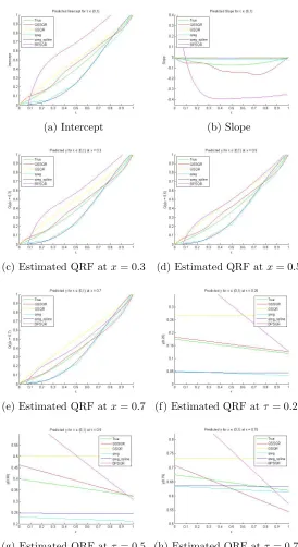
In Section 2.2, we note that after some monotonic transformation, every quantile regres-sion function can be represented in the form mentioned in Equation (2.3). For simulation purposes, we consider two different true quantile functions structure. For each cases, we compare the true and the estimated values of the slope, intercept and the quantile regres-sion function for x= 0.2,0.5 and 0.7, τ = 0.25,0.5 and 0.75 for sample size n = 100 by our proposed methods, Gaussian SQR (GSQR) proposed in Tokdar and Kadane (2012), Bernstein polynomial SQR (BPSQR) proposed in Reich et al. (2011) and qreg and
Reich (2012); Reich and Smith (2013) for details).
For our proposed methods, suppose 0 = t0 < t1 < . . . < tk = 1 be the equidistant knots on the interval [0,1] such thatti = 1/kfor alli= 0,1, . . . , k. Since MCMC does not mix very well for large values ofk, we considered only first 8 possible values ofk for either cases (D = {3,4, . . . ,10} for QSSQR and D ={5,6, . . . ,12} for CSSQR). The value of
r was taken to be 1.25 and it is observed that for this value of r, acceptance ratio stays between 0.25 to 0.45 for most of the cases. Separately, for quadratic and cubic B-spline methods, for each of the values of k, we run 20000 iterations with 5000 burn-in. For QSSQR, while evaluating likelihood, we can solve (2.6) analytically very fast. Although CSSQR can also be solved analytically, we note that the procedure is considerably slower than the bisection method. We apply the latter method with precision of 2−10 ≈ 10−3, after finding the interval whereyi is located fori= 1, . . . , n, by linear search.
To calculate the marginal likelihood of each model, we need to calculate the expression given by Equation (2.16). To calculate the numerator of that term, we considered the last 5000 iterations and we take ω∗ = ({γj(l)}k+mj=1 −1,{δj(l)}k+mj=1 −1) for l = 15000 where
β(l) denotes the l-th update of the parameter β in MCMC. Thus the numerator term is evaluated by the end of MCMC chain. To calculate the denominator term, we consider 5000 draws of{ω(j)}fromq(ω∗, ω|y). Then we computed the marginal likelihoods of each
model. We also computed the estimates corresponding to weighted average quadratic and cubic spline models taking the weights proportional to the marginal likelihoods over the domain of values of k. We used parallel computing for different values of k to obtain posterior probabilities.
To implement the GSQR (Gaussian process SQR) method, proposed in Tokdar and Kadane (2012), we took M = 101 equidistant knots over the interval [0,1], the starting and the ending knots being at 0 and 1 respectively. At each iteration step, we save the values of the Gaussian process at those knots and use those values for likelihood evalu-ations. We ran 20000 iterations with 5000 burn-in. We evaluate the likelihood function by solving (2.6) for each data-points using Newton-Raphson method, as mentioned in Tokdar and Kadane (2012). We took the precision for convergence criteria to be 10−3.
While estimating the quantile regression (QRF) functions using the functions qreg
used for this method is available at the following link1.
For our proposed method, we calculate the uniform 95% posterior credible region for the quantile regression function (QRF) Q(τ|x), τ ∈[0,1] for three distinct co-variate valuesx= 0.2,0.5,0.7 forτ ∈[0,1] for three different sizes of samplen= 50,100 and 200. To find the 95% posterior credible region for the QRF for a given co-variate value using Empirical Bayes method, we calculate the posterior mean of the estimated QRF for all
τ ∈[0,1] for each value ofk ∈Dat that given covariate valueX =x. Since we run 20000 iterations with burn-in 5000, only last H = 15000 are used for calculating the posterior mean. For a given k ∈ D and covariate value X = x, define REB
(x,k) = {a 1
(x,k), . . . , a H (x,k)} such that
ai(x,k)= sup τ∈[0,1]
Q(i)(τ|x, k)−Qˆy(τ|x, k)
, i= 1, . . . ,15000
where Q(i)(τ|x, k) denotes the QRF for X =x in the i-th iteration after burn-in for B-spline method withkpartitions and ˆQy(τ|x, k) denotes the posterior mean of the QRF for
X =xfor B-spline method with k partitions. After that we calculate the 95th percentile of REB
(x,k) for each k ∈ D. Thus we find the size of the 95% posterior credible region for each value of k ∈ D. To find the coverage, we repeat the simulation study 1000 times under different random number seeds and count the number of times the distance of the true QRF from the estimated EB estimate for all τ ∈[0,1] is not more than the size of the 95% posterior credible region for EB approach of correspondingk.
In the HB method, we again have 20000 iterations with burn-in 5000 and only last
H = 15000 are used for calculating the posterior mean. To find the 95% posterior credible region for the QRF for a given co-variate value X =x in this case, we calculate RHB
(x) = {a1
(x), . . . , a H
(x)} such that
ai(x)= sup τ∈[0,1]
Q(i)(τ|x)−Qˆy(τ|x)
, i= 1, . . . ,15000,
whereQ(i)(τ|x) denotes the QRF forX=xin thei-th iteration after burn-in for B-spline method and ˆQy(τ|x) denotes the posterior mean of the QRF for X = x for B-spline method. The weights corresponding to each k∈D to find Q(j)(τ|x) and ˆQ
y(τ|x) are the same and they are derived as mentioned in Section 2.3.3. Then we find the size of the 95% posterior credible region by calculating the 95th percentile of RHB
(x). To find the coverage, we repeat the simulation study 1000 times under different random number seeds and count the number of times the distance of the true QRF from the estimated HB estimate
1
for all τ ∈ [0,1] is not more than the size of the 95% posterior credible region for HB approach.
It is well-known that posterior credible band of smooth functions have an under cover-age property (see Cox (1993); Knapik et al. (2011); Szabo et al. (2015); Yoo and Ghosal (2016)). To alleviate the problem, undersmoothing or modifying the credible region is needed. We inflate the obtained credible region by blowing the radius of the region by a slowly increasing factor. We choose the inflation factor f(n) = 0.8√logn in our exam-ples. This works for all the sample sizes n = 50,100 and 200 under different simulation settings and different true quantile regression functions. We report two simulation studies in this chapter described in Section 2.5.1 and 2.5.2. We have also provided the posterior coverage with and without inflation of uniform 95% posterior credible interval for three different sample sizes under two different true quantile regression functions.
First Study
Consider Q(τ|x) =xξ1(τ) + (1−x)ξ2(τ) where
ξ1(τ) = (1−A)τ2+Aτ, ξ2(τ) = (1−B)τ2+Bτ
and A = 0.3, B = 0.6. We note that ξ1 and ξ2 are strictly increasing function from [0,1] to [0,1] satisfying ξ1(0) = ξ2(0) = 0 and ξ1(1) = ξ2(1) = 1. Note then the conditional quantile function is given byQ(τ|x) =a(x)τ2+b(x)τwherea(x) = x(1−A)+(1−x)(1−B) and b(x) = xA+ (1−x)B. Observe that since the quantile function is the inverse of the cumulative distribution function, for U ∼ U(0,1) the random variable Q(U|x) has conditional quantile function Q(τ|x). We generate n values x1,· · · , xn of the predictor variable X independently from U(0,1). Then we simulate Y variable from the following equation
Yi =aiUi2+biUi for all i= 1, . . . , n
where ai =xi(1−A) + (1−xi)(1−B), bi =xiA+ (1−xi)B and Ui’s are i.i.d. U(0,1),
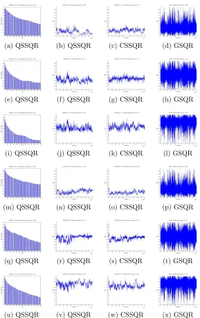
CSSQR approaches under all the considered values of k using 10 identical chains under different random number generator seeds in each cases. It is noted that out of 96 observed GR statistics (QSSQR and CSSQR for D = {3, . . .10} and {5, . . . ,12} respectively, 6 statistics in each case), in 64 cases (about 67%), the GR statistics stays between 1.00 and 1.10 and the highest observed value of the GR statistics is 1.48.
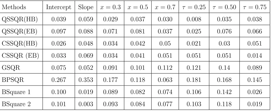
The comparative study of the performances in estimation of our method with other methods under this simulation study has been provided in Figure 2.1. We found that there is not much difference between the estimates given by quadratic and cubic B-spline approaches. Hence, for convenience, we only compared the output of our Hierarchical Bayes QSSQR method with other proposed methods in these figures. The root mean integrated squared error (RMISE) is given by the square root of the average of the square of the differences of the estimated and the true values of the curves at those grid points. In Table 2.1, we compared the RMISE for above mentioned estimated curves for all methods. It can be noted that in our simulation study, the estimated slope, intercept, quantile regression function for x = 0.2,0.5,0.7 and τ = 0.25,0.5,0.75 are curves on the domain [0,1]. To calculate the RMISE, we divide the interval [0,1] using partition (t0, t1, . . . , t100) such that 0 = t0 < t1 < · · · < t100 = 1 such that (ti −ti−1) = 0.01 for all i= 1, . . . ,100. We note that our proposed methods have lower RMISE of estimation curves than that of GSQR. Among other methods, qreg function from BSquare worked quite good, though our method yields lower RMISE values for most of the cases. Among our set of proposed methods, we do not see any noticeable improvement by using CSSQR instead of QSSQR. We note that the HB approach has lower RMISE values than the corresponding EB alternative.
In Table 2.2, we present estimation accuracy and coverage with and without inflation of the proposed methods for three different sample sizes n = 50,100,200. We note that the posterior coverage of the inflated credible band for the Hierarchical Bayes are typi-cally better than that of corresponding Empirical Bayes. No noticeable improvement is observed by using CSSQR instead of QSSQR.
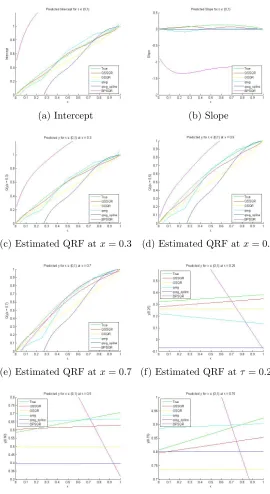
Second Study
To check the performance of the proposed Bayesian method when the quantile function is not a polynomial, we consider,
ξ1(τ) = sin(
πτ
2 ), ξ2(τ) =
(a) Intercept (b) Slope
(c) Estimated QRF atx= 0.3 (d) Estimated QRF atx= 0.5
(e) Estimated QRF atx= 0.7 (f) Estimated QRF atτ= 0.25
(g) Estimated QRF atτ = 0.5 (h) Estimated QRF atτ = 0.75
(a) QSSQR (b) QSSQR (c) CSSQR (d) GSQR
(e) QSSQR (f) QSSQR (g) CSSQR (h) GSQR
(i) QSSQR (j) QSSQR (k) CSSQR (l) GSQR
(m) QSSQR (n) QSSQR (o) CSSQR (p) GSQR
(q) QSSQR (r) QSSQR (s) CSSQR (t) GSQR
(u) QSSQR (v) QSSQR (w) CSSQR (x) GSQR
Table 2.1: (First Simulation study) Comparison of RMISE of estimation of slope, in-tercept and quantile regression function at x = 0.3,0.5,0.7, τ = 0.25,0.50,0.75 and
n= 100 under different methods QSSQR(HB); QSSQR(EB); CSSQR(HB); CSSQR(EB); GSQR; BPSQR; BSquare 1 and BSquare 2 (denoteqregandqreg splinefunction under
BSquarepackage in R respectively)
Methods Intercept Slope x= 0.3 x= 0.5 x= 0.7 τ = 0.25 τ = 0.50 τ = 0.75
QSSQR(HB) 0.039 0.059 0.029 0.037 0.030 0.008 0.035 0.038
QSSQR(EB) 0.097 0.088 0.071 0.081 0.037 0.025 0.076 0.066
CSSQR(HB) 0.026 0.048 0.034 0.042 0.05 0.021 0.03 0.051
CSSQR (EB) 0.033 0.069 0.034 0.041 0.051 0.051 0.051 0.014
GSQR 0.075 0.052 0.091 0.101 0.112 0.121 0.14 0.089
BPSQR 0.267 0.353 0.177 0.118 0.063 0.181 0.168 0.145
BSquare 1 0.100 0.019 0.089 0.082 0.074 0.106 0.142 0.026
BSquare 2 0.101 0.003 0.093 0.084 0.077 0.103 0.118 0.019
again, we note thatξ1 andξ2 are strictly increasing function from [0,1] to [0,1] satisfying
ξ1(0) =ξ2(0) = 0 andξ1(1) =ξ2(1) = 1. We generate a sample of sizen = 100 using the quantile function given by
Q(τ|x) = xξ1(τ) + (1−x)ξ2(τ).
In this case, the assumptions, precision, prior model parameter values, number of itera-tions and burn-in have been taken to be the same as the previous study for all above-mentioned models. The highest and the lowest observed value of the acceptance ratios under in this simulation study are noted to be 0.18 and 0.55 respectively. Similar to the first simulation study, GR statistics are calculated forξ1(τ) andξ2(τ) atτ = 0.25,0.5,0.75 using 10 identical MCMC chains under different random number generator seeds for all the cases. For this simulation study, out of 96 cases, 66 observed GR statistics are between 1.00 and 1.10 and the highest observed value is 1.50.
Table 2.2: (First Simulation study) Size and posterior coverage of inflated (in bold) and regular uniform 95% posterior credible interval of estimated quantile regression function for x = 0.2,0.5,0.7 for τ ∈ [0,1] for three different sizes of sample n = 50,100,200 for QSSQR(HB), QSSQR(EB), CSSQR(HB) and CSSQR(EB).
Degree Samplesize Type Sizex= 0Coverage.2 Sizex = 0Coverage.5 Sizex= 0Coverage.7
QSSQR
n= 50 HB
0.2394 0.1513 99.7 86.1 0.1936 0.1224 99.3 77.5 0.2020 0.1277 98.3 75.1 EB 0.23270.1471 95.970.4 0.19350.1223 94.263.8 0.22100.1397 94.467.3
n= 100 HB
0.1925 0.1121 96.6 57.2 0.1734 0.1010 98.1 56.3 0.2158 0.1257 99.4 74.6 EB 0.23910.1393 97.267.1 0.20790.1211 97.866.7 0.22700.1322 96.667.4
n= 200 HB
0.2094 0.1137 98.8 61.2 0.1727 0.0938 98.1 41.7 0.2066 0.1122 99.2 58.6 EB 0.22960.1247 96.965.0 0.18030.0979 92.747.5 0.19940.1083 93.751.0
CSSQR
n= 50 HB
0.2475 0.1564 99.8 86.5 0.2109 0.1333 99.7 78.1 0.2225 0.1406 99.8 78.4 EB 0.23610.1492 97.768.7 0.19940.1260 95.860.7 0.19300.1220 92.150.7
n= 100 HB
0.2316 0.1349 98.9 68.9 0.1775 0.1034 95.9 41.0 0.1952 0.1137 95.7 49.6 EB 0.21680.1263 95.861.5 0.17680.1030 94.546.3 0.18820.1096 92.746.0
n= 200 HB
0.1978 0.1074 94.8 34.2 0.1749 0.0950 92.7 20.6 0.2088 0.1134 97.8 40.4 EB 0.19210.1043 92.938.7 0.17290.0939 92.229.2 0.19110.1038 93.537.6
coverage with and without inflation using both quadratic and cubic splines are given. In this case also, the proposed methods yield lower RMISE than other methods. Again, no noticeable improvement on using CSSQR over QSSQR has been observed in this scenario also. Like in the previous study, the HB method has lower RMISE values and higher posterior coverage than the corresponding EB method.
as expected. For simulation purposes, all these codes have been written in MATLAB. Simulations have been performed in a cluster with DELL R815 Quad Processor AMD Opteron 16 core 2.3 GHz machines with 512GB RAM, each running 64Bit Fedora Core 20.
Table 2.3: (Second Simulation study) Comparison of RMISE of estimation of slope, intercept and quantile regression function atx= 0.2,0.5,0.7,τ = 0.25,0.50,0.75 andn= 100 under different methods. QSSQR(HB); QSSQR(EB); CSSQR(HB); CSSQR(EB); GSQR; qreg;qreg spline and BPSQR.
Methods Intercept Slope x= 0.2 x= 0.5 x= 0.7 τ = 0.25 τ = 0.50 τ = 0.75 QSSQR(HB) 0.022 0.060 0.020 0.029 0.038 0.037 0.027 0.043 QSSQR(EB) 0.044 0.078 0.032 0.023 0.028 0.011 0.039 0.034 CSSQR(HB) 0.025 0.055 0.029 0.040 0.049 0.031 0.036 0.060 CSSQR(EB) 0.035 0.064 0.042 0.055 0.066 0.060 0.059 0.068 GSQR 0.063 0.089 0.081 0.108 0.126 0.091 0.152 0.135
qreg 0.071 0.068 0.070 0.074 0.080 0.185 0.014 0.042
qreg spline 0.849 0.091 0.860 0.868 0.873 0.551 0.286 0.082
BPSQR 0.317 0.328 0.235 0.112 0.035 0.169 0.196 0.182
Application to Hurricane Intensity Data
Elsner et al. (2008) argued that the strongest hurricanes in the North Atlantic basin have gotten stronger over the last couple of decades. We apply our method to the hurricane intensity data2 in the North Atlantic basin during the period 1981–2006. We use the weighted quadratic spline procedure, i.e., QSSQR(HB).
To use QSSQR(HB), we first mapped the explanatory variable years to the interval [0,1] by change of scale and origin. In this case, we map the year 1981 to 0 and the year 2006 to 1. To map the response variable, the wind speed of the hurricanes at their maximum to the interval [0,1], we assumed that the velocities of the cyclone are coming from a Pareto distribution. The form of the power-Pareto density is given by
f(y) = ak(y/σ) k−1
σ(1 + (y/σ)k)(a+1) y >0
Similar to Tokdar and Kadane (2012) we fix the values of the parameters as a = 0.45,
(a) Intercept (b) Slope
(c) Estimated QRF atx= 0.3 (d) Estimated QRF atx= 0.5
(e) Estimated QRF atx= 0.7 (f) Estimated QRF atτ= 0.25
(g) Estimated QRF atτ = 0.5 (h) Estimated QRF atτ = 0.75
Table 2.4: (Second Simulation study) Size and posterior coverage of inflated (in bold) and regular uniform 95% posterior credible interval of estimated quantile regression func-tion for x = 0.2,0.5,0.7 for τ ∈ [0,1] for three different sizes of sample n = 50,100,200 for QSSQR(HB), QSSQR(EB), CSSQR(HB) and CSSQR(EB).
Degree Samplesize Type Sizex= 0Coverage.2 Sizex = 0Coverage.5 Sizex= 0Coverage.7
QSSQR
n= 50 HB
0.2755 0.1741 100 93.3 0.2149 0.1358 99.3 83.7 0.2315 0.1463 98.9 81.4 EB 0.25140.1589 97.676.9 0.21570.1363 96.569.4 0.24830.1569 96.270.4
n= 100 HB
0.2421 0.1410 99.9 83.2 0.1894 0.1103 99.1 67.3 0.2127 0.1239 98.8 70.4 EB 0.19970.1163 93.455.5 0.18150.1057 93.853.2 0.23490.1368 96.865.7
n= 200 HB
0.1701 0.0924 95.1 39.6 0.1539 0.0836 94.1 26.6 0.1926 0.1046 98.9 48.8 EB 0.19210.1043 93.851.7 0.18560.1008 95.150.5 0.21750.1181 96.458.0
CSSQR
n= 50 HB
0.2563 0.1620 100 89.5 0.1880 0.1188 98.6 59.4 0.1935 0.1223 96.4 51.4 EB 0.26090.1649 98.884.4 0.17720.1120 89.743.7 0.20250.1280 89.846.2
n= 100 HB
0.2010 0.1171 96.0 54.2 0.1636 0.0953 92.5 29.9 0.2201 0.1282 99.1 59.8 EB 0.21920.1277 96.463.0 0.17550.1022 92.742.5 0.22090.1287 97.657.9
n= 200 HB
0.1897 0.1030 94.6 33.0 0.1698 0.0922 92.3 19.6 0.2048 0.1112 96.8 40.4 EB 0.20510.1114 95.146.6 0.17770.0965 92.235.8 0.22040.1197 97.357.2
σ = 52 and k = 4.9. The distribution function is given by
F(y) = 1− 1
(1 + (y/σ)k)a (2.20)
Using Equation (2.20), we transform the hurricane wind speeds to the percentile values. Now, transformed y-values are well in the [0,1] interval and then apply the QSSQR(HB) method. After we evaluate our estimated quantile functions ˆξ1(τ) and ˆξ2(τ), we find out the slope and intercept at functions of τ.
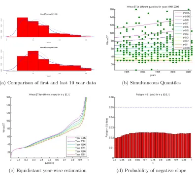
(a) Comparison of first and last 10 year data (b) Simultaneous Quantiles
(c) Equidistant year-wise estimation (d) Probability of negative slope
Table 2.5: Computation time (in seconds) of QSSQR, CSSQR and GSQR for simulation study 1 and 2 with sample size n= 100.
Methods QSSQR CSSQR GSQR
Study 1 672 776 1479
Study 2 666 902 1566
In the data, WmaxST stands for the velocity of the cyclones. In Figure 2.4a, we note that the higher velocity cyclones are more frequent in the period 1997–2006 period than 1981–1990 period. We show the estimates for different quantiles over the period 1981– 2006 in Figure 2.4b by using QSSQR (HB). We note that, the the quantile regression curves (QRF) are more steeper for higher quantiles than the lower quantiles.
In order to check whether really the strongest tropical cyclones in the North Atlantic basin have gotten stronger over the last couple of decades (argued by Elsner et al. (2008)), we draw the estimated velocities as a function of quantiles for the years 1981, 1986, 1991, 1996, 2001 and 2006 in Figure 2.4c. We note that, for these 6 equidistant years, the estimated WmaxST corresponding to the lower quantiles are not pretty much different. While, at higher quantiles, the estimated WmaxST has an increasing trend with time,i.e., more recent years has estimated WmaxST more than the older years for higher quantiles. In Figure 2.4d, we show the posterior probabilities of the slope to be negative at the higher quantiles, i.e., for τ ∈[0.5,1].
Application to US Population Data
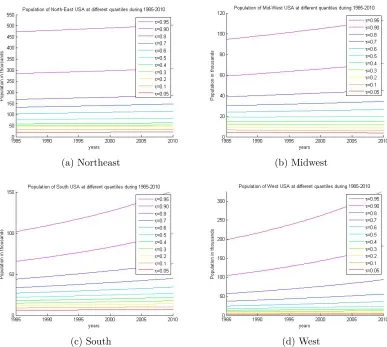
For last few decades, the population of the states of USA are changing. But the rate of change of population is not the same over all zones of USA. We can divide the whole USA mainly in 4 regions namely Northeast, Midwest, South and West. Due to the current trend of globalization, the rate of change of population over the time is different for all these regions of USA. We apply the QSSQR(HB) method of simultaneous quantile regression on the population data3of USA over the period 1985–2010. We use the USGS data where we can found population of each county of USA for the years 1985, 1990, 1995, 2000, 2005 and 2010.
Before applying our method, we did a monotone transformation so that both predictor and response variables lie in between 0 and 1. We transform the years to the unit interval via linear transformation so that the year 1985 gets mapped to 0 and the year 2010
3Source
gets mapped to 1. For the transformation of the population, we considered, the county-wise population of each region follows log-normal density. We fit log-normal density to each of these regions separately. Then for each region, for each county, we use the cumulative distribution function of the population according to the corresponding log-normal distribution. After transforming both explanatory and response variables into the unit interval, we did our analysis. After our analysis we transform the results back to the original scale via the inverse transformation.
(a) Northeast (b) Midwest
(c) South (d) West
Figure 2.5: Estimated quantile curves of county wise population of Northeast, Midwest, South and West regions of USA for the quantilesτ ∈ {0.05,0.10,0.20, . . . ,0.80,0.90,0.95} over the years 1985–2010.
(a) Northeast (b) Midwest
(c) South (d) West
Figure 2.6: Estimated population for τ ∈ [0,1] of Northeast, Midwest, South and West regions of USA for the years 1985, 1990, 1995, 2000, 2005 and 2010
quantile regression function curve of population for τ ∈ [0,1] for the years 1985, 1990, 1995, 2000, 2005 and 2010 for all regions.


![Figure 2.6: Estimated population for τ ∈ [0, 1] of Northeast, Midwest, South and Westregions of USA for the years 1985, 1990, 1995, 2000, 2005 and 2010](https://thumb-us.123doks.com/thumbv2/123dok_us/1241676.1156776/58.612.119.506.77.423/figure-estimated-population-northeast-midwest-south-westregions-years.webp)
![Figure 2.7: Estimated probability of negative slope for τ ∈ [0, 1] of Northeast, Midwest,South and West regions of USA for the years 1985, 1990, 1995, 2000, 2005 and 2010](https://thumb-us.123doks.com/thumbv2/123dok_us/1241676.1156776/59.612.115.506.79.423/figure-estimated-probability-negative-northeast-midwest-south-regions.webp)
