Comparing Technology Adoption Forecasts Generated by an Agent-Based Model and a Scaled and Adjusted Random Utility Model.

EDWARDS, KRISTA ELIZABETH. Comparing Technology Adoption Forecasts Generated by an Agent-Based Model and a Scaled and Adjusted Random Utility Model. (Under the direction of Dr. Scott Ferguson.)

Technology adoption has been previously forecasted using agent-based models that offer

flexible model architecture capable of explicitly representing the effects of both technical and

nontechnical attributes. Even with the capabilities of agent-based modeling, it is difficult to

gather the necessary data to represent the market of a technology and to represent the effects

of nontechnical attributes within the model. This makes it worthwhile to search for a model

form that requires less information and less modeling of hard-to-capture effects. This

research evaluates the adoption forecasts generated by a scaled and adjusted random utility

model that explicitly represents only the effects of technical attribute preferences against

those of an agent-based model. This research also develops an agent-based model with a

unique social network construction procedure. The effects of the social network model

parameters on the resultant adoption forecasts are explored. The presented results indicate the

format of a scaled and adjusted RUM that is needed to generate adoption forecasts

comparable to those of an agent-based model. The presented results also that for the social

network used in this work, the social network rewiring probability that creates the structure

© Copyright 2017 by Krista Elizabeth Edwards

Comparing Technology Adoption Forecasts Generated by an Agent-Based Model and a Scaled and Adjusted Random Utility Model

by

Krista Elizabeth Edwards

A thesis submitted to the Graduate Faculty of North Carolina State University

in partial fulfillment of the requirements for the degree of

Master of Science

Mechanical Engineering

Raleigh, North Carolina

2017

APPROVED BY:

_______________________________ _______________________________ Dr. Joe DeCarolis Dr. Brendan O’Connor

_______________________________ Dr. Scott Ferguson

DEDICATION

This thesis is dedicated to my parents Frank and Marie Edwards, who have done more for my

education mentally, emotionally, and financially for more than 24 years than any child ever

BIOGRAPHY

Krista Edwards completed her Bachelor of Science degree in Mechanical Engineering and

Minor in Mathematics at Clemson University in May of 2015. Upon graduation, she enrolled

at North Carolina State University to pursue a Master of Science degree in Mechanical

Engineering in the fall of 2015 as a fourth generation student. Krista immediately joined the

System Design Optimization Lab and began working towards the completion of her thesis

ACKNOWLEDGMENTS

The author expresses her appreciation for her advisor, Dr. Scott Ferguson for his support and

the opportunity to pursue a Master of Science degree at North Carolina State University. The

author would also like to thank her lab-mates Charlotte Lawrence, Samantha White, Kevin

Young, Rachel Hough, Anya Flowe, Gordon T. Beverly III, Jaekwan Shin, and her cat Kirby

for their assistance and unwavering support during her time in the System Design

Optimization Lab. The author also recognizes the support of the National Science Foundation

for funding this work through NSF CAREER Grant No. CMMI-1054208. Any opinions,

findings, and conclusions presented in this paper are those of the authors and do not

TABLE OF CONTENTS

LIST OF TABLES...x

LIST OF FIGURES ... xi

CHAPTER 1 – INTRODUCTION ... 1

1.1 Introduction ... 1

1.2 Research Questions ... 2

1.3 Consumer Choice Modeling... 6

1.4 Simulation Topic: Residential Solar Systems ... 8

1.5 Chapter Summary ... 9

CHAPTER 2 – BACKGROUND ... 10

2.1 Introduction ... 10

2.2 Agent-Based Modeling of Adoption ... 11

2.3 Modeling the Consumer Choice to Adopt... 13

2.4 Social Network Modeling ... 19

2.5 Chapter Summary ... 22

CHAPTER 3 – RESEARCH QUESTION 1 METHODOLOGY ... 24

3.1 Introduction ... 24

3.2 Exploration of the Effects of Social Network Parameters on Adoption Forecasts .. 24

3.3 Agent-Based Model Development ... 25

CHAPTER 4 – SIMULATION OF ROOFTOP RESIDENTIAL SOLAR SYSTEM ADOPTION IN CARY, NC ... 35

4.1 Motivation ... 35

4.2 Selection of Simulation Neighborhoods ... 35

4.3 Selection of Technical Attributes and Levels ... 36

4.4 Agent Creation for the Agent-Based Model ... 39

4.5 Part-Worth Addition Values... 48

CHAPTER 5 – RESEARCH QUESTION 1 RESULTS AND DISCUSSION ... 52

5.1 Introduction ... 52

5.2 Determining the Effect of Social Influence Necessary to Change Adoption Decisions ... 52

5.4 Research Question 1: Effect of Social Network Modeling Parameters on Simulation

Adoption Forecasts ... 60

5.5 Exploring the Effects of the Social Influence Part-Worth on Adoption Forecasts .. 61

5.6 Effect of the Average Number of Connections on Adoption ... 65

5.7 Effect of the Percentage of Connections that are Strong on Adoption ... 66

5.8 Effect of the Social Network Rewiring Probability on Adoption ... 67

5.9 Chapter Summary ... 69

CHAPTER 6 – RESEARCH QUESTION 2 METHODOLOGY ... 70

6.1 Introduction ... 70

6.2 Scaled and Adjusted Random Utility Model of Adoption ... 70

6.3 CBC Survey Responses for the Scaled and Adjusted RUM ... 74

6.4 Formulations of the Scaled and Adjusted RUM ... 75

CHAPTER 7 – RESEARCH QUESTION 2 RESULTS AND DISCUSSION ... 78

7.1 Introduction ... 78

7.2 Scaled and Adjusted RUM – Method 1 ... 79

7.3 Scaled and Adjusted RUM – Method 2 ... 84

7.4 Scaled and Adjusted RUM – Method 3 ... 89

7.5 Interpreting the Forecasts of the Scaled and Adjusted RUM Using Method 3 ... 95

CHAPTER 8 – CONCLUSIONS ... 97

8.1 Research Overview ... 97

8.2 Research Question 1 ... 98

8.3 Research Question 2 ... 99

8.4 Future Work ... 100

REFERENCES ... 102

APPENDIX A: SIMULATION NEIGHBORHOODS IN CARY, NC ... 112

APPENDIX B: DEMOGRAPHIC AVERAGES AND STANDARD DEVIATIONS FOR EACH SIMULATION NEIGHBORHOOD ... 117

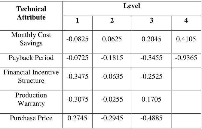
APPENDIX C: MEAN PART-WORTHS FOR TECHNICAL ATTRIBUTE LEVELS FOR EACH AGENT CLASS ... 118

APPENDIX D: PAYBACK PERIODS OF VARYING SYSTEM SIZES AND FINANCIAL INCENTIVES APPLIED ... 120

APPENDIX F: COMPLETE DATA FOR ADOPTION FORECASTS GENERATED

USING THE SCALED AND ADJUSTED RUM ... 126

F.1. Forecasts Generated Using Optimization Method 1 ... 126

F.2. Forecasts Generated Using Optimization Method 2 ... 128

LIST OF TABLES

Table 2.1: Comparison of Agent-based models found in this work and existing works ... 13

Table 2.2: Hypothetical attributes and levels for product Z ... 16

Table 4.1: Attributes and levels chosen to represent residential solar systems ... 37

Table 4.2: Mean part-worths for group 3: majority adopters... 41

Table 4.3: Residential solar panel specifications ... 44

Table 3.1: Probability of adoption to be covered by social influence at each iteration ... 55

Table 5.2: Model parameter values used in the simulation ... 58

Table 5.3: Frequency of each monthly cost savings attribute level as a result of the agent-specific system optimizations ... 58

Table 5.4: Frequency of each payback period attribute level as a result of the agent-specific system optimizations ... 59

Table 5.5: Relative increases [%] in forecasted adoption at the 10th iteration for selected social influence part-worth values ... 64

Table 5.6: Relative increases [%] in forecasted adoption at the 20th iteration for selected social influence part-worth values ... 64

Table 5.7: Relative increases [%] in forecasted adoption at the 30th iteration for selected social influence part-worth values ... 65

Table 6.1: Description of the three methods used to optimize 𝑠 and 𝜂 ... 76

Table 7.1: Binary logit fit – technical attribute part-worths and intercept... 79

Table 7.2: Optimized scaling and adjustment parameters – Method 1 ... 84

Table 7.3: Optimized scaling and adjustment parameters – Method 2 ... 88

Table 7.4: Evolution of 𝑠 and 𝜂 using the scaled and adjusted RUM – method 3 – forecasting one iteration before re-optimizing ... 92

LIST OF FIGURES

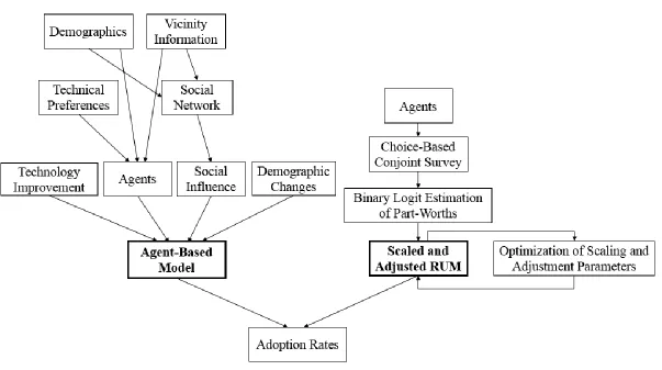
Figure 1.1: Overview of the agent-based model and the scaled and adjusted RUM ... 5

Figure 2.1: Overview of this chapter’s content relevant to the goals of this research ... 10

Figure 2.2: Hypothetical choice task for variations of product Z ... 17

Figure 3.1: Framework of the Agent-Based Model ... 26

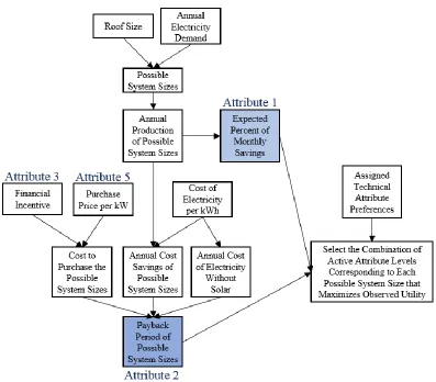
Figure 4.1: Process of optimizing each agent’s system configuration... 43

Figure 4.2: Map of expected kWh produced per kW-year [75] ... 45

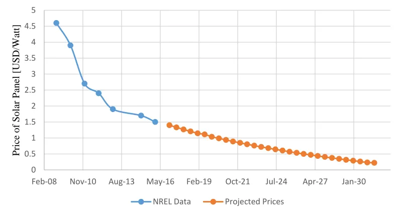
Figure 4.3: Historical (blue) and projected (orange) data on the price of solar systems ... 50

Figure 4.4: Historical (blue) and projected (orange) data on the cost of electricity ... 50

Figure 5.1: Flow of the discussion in this section ... 57

Figure 5.2 Adoption of residential solar systems in Cary, NC ... 59

Figure 5.3: Adoption forecasts at varying values of 𝛽𝑆𝐼 ... 62

Figure 5.4: Number of agents that adopt at varying values of 𝛽𝑆𝐼 ... 63

Figure 5.5: Adoption forecasts at varying values of 𝑐 ... 66

Figure 5.6: Adoption forecasts at varying values of 𝑝𝑠 ... 67

Figure 5.7: Adoption forecasts at varying values of 𝛼 ... 68

Figure 6.1: Flow of the discussion in this section ... 71

Figure 6.2: Framework of the scaled and adjusted RUM ... 72

Figure 7.1: Flow of the discussions in this chapter ... 78

Figure 7.2: Adoption forecast – Scaled and adjusted RUM – Method 1 – Two ABM forecasted adoption data points ... 80

Figure 7.3: Adoption forecast – Scaled and adjusted RUM – Method 1 – Three ABM forecasted adoption data points ... 80

Figure 7.4: Adoption forecast – Scaled and adjusted RUM – Method 1 – Ten ABM forecasted adoption data points ... 81

Figure 7.5: Adoption forecast – Scaled and adjusted RUM – Method 1 – Five ABM forecasted adoption data points ... 81

Figure 7.6: Adoption forecast – Scaled and adjusted RUM – Method 1 – Six ABM forecasted adoption data points ... 82

Figure 7.7: Adoption forecast – Scaled and adjusted RUM – Method 1 – Seven ABM forecasted adoption data points ... 82

Figure 7.8: Observed utility - Scaled and adjusted RUM – Method 1 – Three ABM forecasted adoption data points ... 83

Figure 7.9: Adoption forecasts – Scaled and adjusted RUM – Method 2 – Varying number of ABM forecasted adoption data points – Excluding two initial ABM forecasted adoption data points ... 85

Figure 7.11: Adoption forecasts – Scaled and adjusted RUM – Method 2 – Two ABM forecasted adoption data points – Excluding a varying number of initial ABM forecasted adoption data points ... 87 Figure 7.12: Adoption forecasts – Scaled and adjusted RUM – Method 2 – Eight ABM forecasted adoption data points – Excluding a varying number of initial ABM forecasted adoption data points ... 87 Figure 7.13: Adoption Forecast – Scaled and adjusted RUM – Method 3 – One iteration forecasted before re-optimizing s and η ... 90 Figure 7.14: Adoption Forecast – Scaled and adjusted RUM – Method 3 – Two iterations forecasted before re-optimizing s and η ... 90 Figure 7.15: Adoption Forecast – Scaled and adjusted RUM – Method 3 – Four iterations forecasted before re-optimizing s and η ... 93 Figure 7.16: Adoption Forecast – Scaled and adjusted RUM – Method 3 – Seven iterations forecasted before re-optimizing s and η ... 93 Figure 7.17: Adoption Forecast – Scaled and adjusted RUM – Method 3 – Nine iterations forecasted before re-optimizing s and η ... 94 Figure 7.18: Observed utility - Scaled and adjusted RUM – Method 3 – One iteration

CHAPTER 1 – INTRODUCTION

1.1 Introduction

Predicting consumer purchase choices, including decisions to adopt a technology for the first

time, has been a topic of study dating back to Thurstone’s analysis of respondent’s

differentiation of psychological stimuli in 1927 [1]. Consumers make technology adoption

decisions not only by considering how well the technical attributes meet their preferences,

but this decision is also influenced by their demographic characteristics, influence from their

friends and neighbors, and other nontechnical attributes [2]. Yet, the effect of mechanisms

like social influence is not fully understood [3]. Also, it is difficult to collect the large-scale

data needed to model a consumer’s social networks. Despite the difficulties of including the

effects of nontechnical attributes in a model, they have a marked effect on adoption decisions

[4,5]. It is therefore worthwhile to develop adoption models that can indirectly account for

the effects of nontechnical attributes, because this can require less information and less

reporting of possibly sensitive information by the respondent.

Agent-based models have gained popularity in modeling consumer choice and adoption [6,7]

by employing heterogeneous agents that use defined behavioral rules to generate individual

adoption decisions [8,9]. Such models allow for the effects of both technical and

nontechnical factors that influence a purchasing decision to be studied. The architecture of an

agent-based model facilitates the exploration of the effects of social influence, a topic whose

mechanics are not completely understood [3]. Connections to other agents can be dictated by

to discover correlations to increases or decreases in forecasted adoption. The agent-based

model’s ability to provide an evaluative standard for other model formulations and to enable

the study of social influence on adoption are leveraged in the research questions driving this

work.

Additionally, this work compares forecasts from an agent-based model against a scaled and

adjusted random utility model (RUM). The scaled and adjusted RUM explicitly models

technical attribute preferences through a binary logit fit of choice-based conjoint survey

responses. The effects of nontechnical attributes are then modeled using scaling and

adjustment parameters that modify the observed utility of a technology as time passes.

1.2 Research Questions

Research Question 1 (RQ1) is driven by our limited understanding of the effect that each

social network model parameter has on adoption forecasts in an agent-based model. If the

network parameters that feed into a certain component of the social network are found to not

have an effect on forecasted adoption, a modeler does not have to spend significant effort

defining proper parameter values.

Research Question 1: What effect does changing the parameters of the social network model have on adoption forecasts generated using an agent-based model?

The importance of considering social influences that affect consumer choice is discussed in

persons to conform to society, including the desire to be similar to friends and those around

you [10]. The decision on whether or not to adopt a technology is not an exception to this

desire. For this reason, recent consumer choice modeling applications have included social

influence as a consumer choice model attribute ([11], for example) that contributes to the

observed utility of the product. A unique component of this research is the model formulation

for social networks used to account for social influence in the consumer choice models. The

social network combines two individual networks independently created based on different

causes of social connections: demographic similarity and physical vicinity or colloquially,

friends and neighbors. The effects of the parameters that the social network model on

forecasted adoptions are explored.

First, the social influence part-worth, 𝛽_𝑆𝐼, representing the magnitude of the effects that social influence has on agents is varied. This is done to determine the magnitude of 𝛽𝑆𝐼 that

allows the effects of the remaining model parameters to be seen. Second, the parameters of

the social network that can be varied are explored to determine which of the social network

parameters have an effect on adoption forecasts.

Research Question 2: What form of a scaled and adjusted random utility model can generate adoption forecasts comparable to those of an agent-based model?

Research Question 2 (RQ2) attempts to determine if a new model form that only explicitly

models the effects of technical attribute preferences can forecast adoption comparable to

those generated by an agent-based model. The new model form, the scaled and adjusted

account for the effects of nontechnical attributes (demographic changes, technology

improvements, and social influence). Three methods of optimizing the scaled and adjusted

RUM parameters are investigated. The purposes and strengths of each method are discussed

as well to guide the decision of which method and what available data should be used in a

specific application.

The form of the scaled and adjusted random utility model (RUM) is shown in Equation (1.1),

where the scaling factor 𝑠 and adjustment factor 𝜂 are the optimized model parameters used to continually modify the observed utility 𝑉 at time 𝑡 for a technology as time passes to indirectly account for changes in a technology’s observed utility due to nontechnical

attributes.

𝑉_𝑡+1 = 𝑠(𝑉_𝑡) + 𝜂 (1.1)

The indirect representation of the effects of nontechnical attributes on forecasted adoption

over time is attempted using scaling and adjustment parameters. The success of these

methods is dependent on finding scaling and adjustment parameters that modify the observed

utility to mimic the effect of nontechnical attributes. Different methods of optimizing the

scaling and adjustment parameters are developed to determine which method(s), if any,

produce similar adoption forecasts as the agent-based model. Figure 1.1 shows an overview

of these two models.

In this research, a simulation in residential rooftop solar system adoption forecasting is used

agent-based model’s flexible architecture to explore the effects of social network model

parameters on adoption forecasts and while the second research question examines the

implications of the success or failure of the scaled and adjusted RUM that explicitly models

only technical attribute preferences.

1.3 Consumer Choice Modeling

Consumer choice models aim to capture and quantify the drivers of the purchase of a product

and use them to predict the choices that consumers will make regarding new technologies

offered in the future. Discrete choice modeling is one consumer choice modeling technique

used to capture consumer preferences for individual aspects of a product by surveying a

sample of the market to collect stated preference data [12] or by fitting models to historical

purchase or adoption data (called using revealed preference data) [13,14]. Stated preference

methods of discrete choice modeling are used in this work for their ability to better represent

hypothetical market conditions [15] and because a new technology will have limited

historical purchase data. Choice-based conjoint (CBC) surveys are often used to collect

stated preference data; they offer the survey taker a choice set of product options and,

usually, the choice to not purchase any of the given products. Responses to CBC surveys are

then used to form mathematical representations of consumer preferences using the concept of

observed utility.

Following the structure of a random utility model [16–19], an observed utility for a

technology is assigned and used to predict the probability the product will be purchased.

alongside other product configurations and/or the option not to purchase, all of which also

have a corresponding observed utility. Observed utility is a dimensionless mathematical

representation of a consumer’s preference for a technology and is the sum of part-worths for

individual technology attributes. Attributes included in consumer choice models can be

technical or nontechnical. Technical attributes of a product are relatively easily identified and

quantified. A simple example of identifying and quantifying a technical attribute of a product

is identifying operating power as an important attribute of a lightbulb, quantified in Watts.

Some nontechnical attributes that can be included in consumer choice models are relevant

demographic information on the consumer(s), usage context for the technology of the

consumer(s), and social influence as done in the work of He et al [11], for example. Equation

(1.2)shows the mathematical representation of consumer 𝑛’s observed observed utility 𝑉 for technology configuration 𝑗, where observed utility is the sum of the products of the consumer’s part-worth 𝛽 for an attribute level and the active attribute level indicator 𝑥. Each technology configuration has 𝐾 attributes, each with a corresponding 𝑘_𝑙 attribute levels.

𝑉_𝑛𝑗 = ∑ ∑ 𝛽_𝑛𝑘𝑙𝑥_𝑗𝑘𝑙

𝑘𝑙

𝑙=1 𝐾

𝑘=1

(1.2)

Equation (1.2) represents observed utility while in actuality, total utility is comprised of

observed utility (captured by discrete choice modeling) and unobserved utility, or error.

Unobserved utility are the result of both irrational purchase decisions and influences not

consumer choice models arise. Popular consumer choice models that exist in literature and in

practice include the logit model [19], the generalized extreme value (GEV) model [20], the

probit model [1,21], and mixed logit model [22,23]. In this research, a form of the logit

model, the binary logit model [24] which considers only two purchase options, is used to

estimate the probability of adoption. A binary logit model is most appropriate for adoption

forecasting since the percentage of adopters in the market is the only figure of consequence.

Therefore, a more complicated model that accounts for more than two choices (i.e. adopt or

not adopt) is not needed. Examples of the use of binary logit models within technology

adoption including the use of a binary logit model to identify key factors in the adoption of

GPS guidance systems by cotton farmers [25], to model the adoption of electronic business

by European countries [26], and to model the choice to telecommute [27]. The binary logit

model in this work is used to generate probabilities of adoption at both the individual and

population level. Determining the probability of adoption using the binary logit model is

discussed further in Section 2.3.

1.4 Simulation Topic: Residential Solar Systems

Adoption forecasts of residential solar systems based on the characteristics of a group of

neighborhoods in Cary, North Carolina is used to explore the research questions introduced

in Section 1.2. Residential solar systems continue to be one of the most commonly installed

forms of residential distributed generation of electricity [28] and is the fastest growing

energy technology in the world [29,30]. Systems are installed to reduce carbon emissions

from the traditional power grid but are installed more commonly to reduce the amount of

a residential solar system that allows the resident to produce, in part, their own power affects

the amount of power needed from the central power grid. In an era where many individuals

are seeking alternate forms of power generation that do not use non-renewable resources

(coal, natural gas, e.g.) [31], considering and planning for the effects of increased usage of

residential solar systems is a worthwhile endeavor.

1.5 Chapter Summary

Chapter 2 provides background information on existing agent-based, consumer choice, and

social network models. Chapter 3 provides the methodology used to explore RQ1, Chapter 4

presents the simulation in residential solar system adoption, and Chapter 5 presents the

results and discussion pertaining to RQ1 and the simulation in residential solar system

adoption. Chapter 6 provides the methodology used to explore RQ2 while Chapter 7 presents

the results and discussion pertaining to RQ2. Chapter 8 gives the conclusions drawn from

this research and avenues for future research. References and Appendices to support this

CHAPTER 2 – BACKGROUND

2.1 Introduction

The fundamentals of agent-based modelling are introduced in the next section of this chapter.

The following two sections of this chapter introduce modelling concepts fundamental to

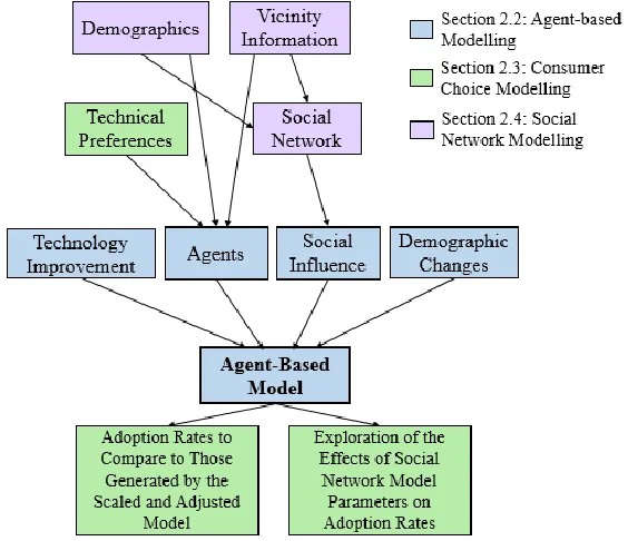
developing the agent-based model. Figure 2.1 depicts how the concepts discussed in this

chapter contribute to the overall goals of this research where the color of the box corresponds

to the content included in the sections of this chapter. The comparison of adoption and the

exploration of social network model parameters on forecasted adoption are not actually

discussed in Section 2.3, but the necessary translation of technical attribute preferences and

nontechnical attribute information into forecasted adoption is.

2.2 Agent-Based Modeling of Adoption

Agent-based modeling (ABM) is growing in popularity for exploring “how the interaction of

heterogeneous agents at the micro-level produces macro outcomes” [6]. ABM is more

flexible than other adoption modeling approaches, such as population-level multinomial logit

modeling, due to its ability to represent complex agents that each have characteristics

(technical attribute preferences, demographics, e.g.), social interactions, and defined behavior

[8,9]. The flexible architecture of ABM lends itself well to modeling technology adoption in

which each potential adopter in the market has heterogeneous preferences and influences. All

ABM follows three general steps: 1) create agents with characteristics, 2) define how these

characteristics will influence behavior using stochastic or deterministic rules, and 3)

aggregate the agents’ behaviors over time so that the outcome of the agent characteristics and

defined behavior rules can be understood [6].

In this work, the ability of an agent-based model to represent individuals with varying

technical attributes preferences and to represent the varied effects of their nontechnical

attributes (social influence, demographic changes over time, and technology improvements

over time e.g.) is leveraged. Technical attributes of the technology are assigned

agent-specific part-worths estimated using CBC survey responses and a binary logit model fit

(Section 2.1). Part-worth additions to the observed utility of the technology represent the

agents’ increased usefulness of the technology that is a result of nontechnical attributes. In

application, the value of the part-worths representative of each nontechnical attribute would

be estimated from responses to CBC questions and accompanying questionnaires on

their significance relative to the other attributes’ part-worths. The individuality of agents in

the agent-based model represents the heterogeneity of consumers present in most markets

and is used to aggregate individual adoption decisions into population-level adoption.

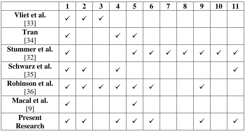
A comparison of other agent-based models used to study the adoption of technology is

summarized in Table 2.1 with an accompanying list of comparison criteria prior to the table.

Table 2.1 shows that this work uses similar ABM components as existing literature; the work

by Stummer et al. [32], however, boasts a very well-developed social network. The social

network in this work could be improved in future work to incorporate some of the additional

elements in Stummer et al.’s work. Though the agent-based model in this research does not

explicitly account for the financial situation of agents, the effect of finances is somewhat

wrapped up in the part-worth additions representing changes in demographics over time, as

income is usually relevant to the purchase of a technology.

1. Considers agent’s technical attribute preferences

2. Considers demographics of agents

3. Considers financial situation of agents

4. Considers how much or how little agents care about environmental effects of their

adopted technology

5. Considers effects of physical vicinity in social network

6. Considers effects of demographic similarity in social network

7. Considers effects of directed connections in social network

9. Uses a small-world social network

10.Considers effects of advertisements and direct experience on adoption

11.Considers how technology and alternative products will change over time

Table 2.1: Comparison of Agent-based models found in this work and existing works

1 2 3 4 5 6 7 8 9 10 11

Vliet et al.

[33]   

Tran

[34]   

Stummer et al.

[32]        

Schwarz et al.

[35]    

Robinson et al.

[36]       

Macal et al.

[9]  

Present

Research       

2.3 Modeling the Consumer Choice to Adopt

Adoption is the decision of a consumer to purchase a technology for the first time.

Forecasting the adoption of a technology requires knowledge of consumers’ preferences for

the technology, or how well available technology satisfies the needs of the consumers,

compared to the consumers’ other choices. This knowledge is needed relative to both the

present and the future, but predicting future choices necessitates anticipating changes in

alternatives, the agent, and the technology itself. In both cases (present and future),

determine the observed utility of a technology and predict consumer choice; this chapter will

provide an explanation of the consumer choice models used in this research.

The methods of discrete choice modeling, introduced in the first chapter, are used in this

research to quantify preferences for a technology to enable forecasting adoption. The

foundations of discrete choice modeling were introduced by Heckman and Dubin and

McFadden [19,37] and further developed by Train [38,39]. The discrete choice model has

been applied to the modeling of technology adoption in literature similar to its use in this

research [15,25,40]. Discrete choice models are rooted in the assumption that the market has

been presented with a choice set consisting of the technology in question and all of its

alternatives that is mutually exclusive, exhaustive, and finite [41].

Despite the possibility that some technology alternatives offered to the consumer may be able

to be used in conjunction (and therefore not be mutually exclusive), assuming that this is not

the case enables modeling the choice to adopt in this manner. From these assumptions, the

probability of market consumers selecting each choice can be derived by then assuming that

consumers are maximizing the observed utility of their purchase. Models derived in this

fashion are called random utility models, introduced by Marschak [16] and developed by

others [42], in which an individual’s (potential adopter’s) utility for a technology is modeled

as a random variable.

The structure of the random utility model is as follows, summarized from the discussion

Assuming the consumer is maximizing the observed utility of the purchase, the consumer

chooses alternative 𝑖 such that 𝑈_𝑛𝑖 is greater than all 𝑈_𝑛𝑗 for all 𝑗 not equal to 𝑖. However, the total utilities 𝑈_𝑛𝑗 of the alternatives is not known to the modeler; only the attributes 𝑥_𝑛𝑗 of the alternatives and the attributes of the consumers 𝑐_𝑛 can be observed. Knowing this, an

observed utility 𝑉𝑛𝑗, a function of 𝑥𝑛𝑗 and 𝑐𝑛, is found. The unobserved percentage of the

total observed utility 𝑈_𝑛𝑗 is captured in a stochastic “error” term 𝜀_𝑛𝑗 so that consumer 𝑛’s observed utility for alternative 𝑗 is the sum of observed utility and unobserved utility

(Equation (2.1)).

𝑈_𝑛𝑗 = 𝑉_𝑛𝑗+ 𝜀_𝑛𝑗 (2.1)

The probability of consumer 𝑛 selecting alternative 𝑖 out of the 𝐽 alternatives is then found by comparing total utilities for the alternatives in question:

𝑃_𝑛(𝑖) = Pr(𝑈𝑛𝑖 ≥ 𝑈𝑛𝑗) = Pr⁡(𝑉𝑛𝑖+ 𝜀𝑛𝑖 ≥ 𝑉𝑛𝑗+ 𝜀𝑛𝑗)

= Pr(𝜀_𝑛𝑗− 𝜀_𝑛𝑖 ≤ 𝑉_𝑛𝑖− 𝑉_𝑛𝑗)for all j≠i.

(2.2)

By assuming different distributions of the error term, multiple consumer choice models arise.

Popular consumer choice models that exist in literature and in practice include the logit

model (extreme value distribution) [19], the generalized extreme value (GEV) model

(generalized extreme value distribution) [43], the probit model (normal distribution) [1,21],

model is used to estimate the probability of adoption. Assuming this distribution and

assuming the error terms are independently and identically distributed across the 𝐽 alternatives and 𝑁 individuals, Equation (2.3) shows the probability of consumer 𝑛 selecting alternative 𝑖 out of the 𝐽 alternatives:

𝑃_𝑛(𝑖) = 𝑒𝑉𝑛𝑖

∑𝐽_𝑗=1𝑒𝑉𝑛𝑗 for all j≠i (2.3)

Estimating the observed percentage of total observed utility necessitates the assumption that

a product can be represented by attributes each with a number of levels. Attributes can be

continuous (e.g. efficiency) or discrete (e.g. material), but defining a reasonable number of

product representative attribute levels requires the discretization of all attributes. An example

of how a product is represented using attributes and levels is given in Table 2.2.

Table 2.2: Hypothetical attributes and levels for product Z

Attribute Level 1 Level 2 Level 3

Efficiency 10% 50% 100%

Material Steel Plastic Aluminum

Shape Round Square Rectangular

The observed percentage 𝑉_𝑛𝑗 of total observed utility 𝑈_𝑛𝑗 is the sum of the products of part-worth estimates 𝛽𝑛𝑘𝑙 and active attribute levels 𝑥𝑗𝑘𝑙 for consumer 𝑛 and product attributes 𝑘

observed utility are commonly estimated using data collected using choice-based conjoint

(CBC) surveys [44].

𝑉𝑛𝑗 = ∑𝐾𝑘=1∑𝐿𝑙=1𝛽𝑛𝑘𝑙𝑥𝑗𝑘𝑙 (2.4)

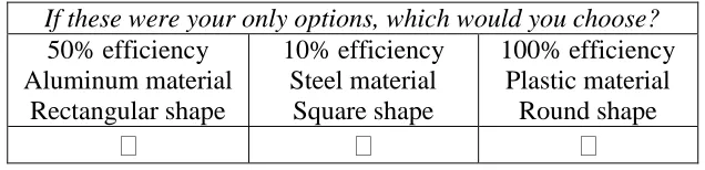
In CBC surveys, respondents are presented with “tasks” each containing a set of hypothetical

product choices to select between, often including the option not to purchase any of the

presented choices (the “outside good” option). Variations on the same product make up the

hypothetical choices where variation is conveyed using the attribute level differences.

Software such as Sawtooth Software CBC SSI Web [45] is often used to create, field, and

analyze CBC surveys so that the process is automated. An example of a CBC survey task is

given in Figure 2.1.

If these were your only options, which would you choose?

50% efficiency Aluminum material

Rectangular shape

10% efficiency Steel material

Square shape

100% efficiency Plastic material

Round shape

Figure 2.1: Hypothetical choice task for variations of product Z

After enough survey responses have been collected part-worths can be estimated using the

logit model. The number of responses needed to obtain a statistically significant result is

dependent on the size of the market population, the homogeneity of the population, the

the discrete choice model was first introduced in 1959 by Luce [17] and further developed by

Block and Marschak [16], Marley (see Luce & Suppes [47]), and McFadden [19]. By using

maximum likelihood estimation (Equation (2.5)) for the aggregate of the CBC survey

responses, an optimized fit of part-worths for each attribute level is found. Here, 𝑁 is the total number of consumers that answered the survey, 𝐽 is the total number of product alternatives included in the survey, and 𝐴 is the total number of part-worths to be estimated (the sum of all product attribute levels minus one zero-encoded part-worth for each product

attributes plus an intercept part-worth).

𝐿𝐿 = ∑ ∑exp⁡(𝑦𝑛𝑗 ∙ (𝛽𝑛0+ 𝛽𝑛1𝑥1+ ⋯ + 𝛽𝑛𝐴𝑥𝐴)) 1 + exp⁡(𝛽𝑛0+ 𝛽𝑛1𝑥𝑛1+ ⋯ + 𝛽𝑛𝐴𝑥𝐴) 𝐽

𝑗=1 𝑁

𝑛=1

(2.5)

As mentioned, a specific form of the logit model will be used in this work. The binary logit

model [24] considers only two product alternatives, and in the case of adoption modeling,

those product alternatives are to adopt the product alternative offered or to not adopt at all.

Equation (2.6) shows the simplification of Equation (2.3) for the probability of adoption of

“product 1” given only the two choices of product 1 and the option not to adopt (the outside

good). It is important to note that the observed utility of the outside good is set to one.

For a successful technology, the percentage of the market that has adopted a technology for

the first time has been shown to in many cases create an S-curve when plotted against time

[48]. The S-curve is a result of slow adoption rates driven almost solely by tech-savvy or risk

taking consumers right after the release of the technology, then a marked increase in adoption

rates once 1) the technology has been proven useful and 2) information about the existence

and usefulness of the technology has spread. Finally, slowed adoption rates are seen after 1)

the majority of consumers that will adopt have adopted and 2) newer and better technology

with the same function has been introduced to the market, either by the same manufacturer or

a competing company.

2.4 Social Network Modeling

A social network is a set of socially relevant nodes connected by one or more relations [49].

A social network is constructed in this research to account for the effects of social influence

on adoption forecasts within the agent-based model. Wasserman and Faust [50] provide a

more in-depth review of social networks and their analysis, but a brief overview is provided

here. In traditional consumer choice models, the influence that friends and neighbors have on

purchase decisions is often not explicitly accounted for. However, [10,51,52] and others have

shown that decisions in most aspects of life, including the purchase of new technologies, are

influenced by what the people around you are doing. The influence of friends and neighbors

on a decision maker’s choice has been explored specifically for the adoption of technology as

well. For example, He et al. [11] explore the addition of a social influence term to the

traditional multinomial logit model in the form of demographic similarity and the “average

California. They found that adding a social influence term improved the quality of the model

as compared to the real data on HEV and conventional car purchases in California. This

study was restricted, however, to accounting for the influence from demographically similar

consumers.

Multiple studies have concluded that influence from those physically nearby is significant.

Discussed here are two studies relevant to the simulation introduced in Chapter 4 which

focus on the highly localized but significant influence of adopters in a potential adopter’s

physical vicinity on the adoption of residential solar systems. First, the work of Bollinger and

Gillingham [53] found that one additional installation of a residential solar system increases

the chance of another installation in the same ZIP code by .78%. In addition, the work of

Rode and Weber [54] found that seed installations could feasibly increase the number of

additional installations in the surrounding kilometer radius by more than one per year. The

significance of localized imitation shown in these works is the reason the effect of physical

vicinity was added into the social network construction model generated in this work.

The generation of network connections due to demographic similarity in this model is based

on the work of He et al. [11] where a discussion of the theoretical foundations of the

following equations can be found. In short, the concept of homophily, or the notion that

friends are generally similar to each other, and the findings of Rogers [55] that homophilous

persons can influence each other, are used to support the claim that demographic similarity is

an appropriate substitute for actual data which individuals in a market are socially connected

the fact that there exist different levels to social connection that are important to consider.

Purchasers are more likely to be influenced by their immediate family and close friends than

by online reviews and acquaintances, for example. To account for this difference in

connection significance, the idea of weak and strong connections is used.

The presence of a connection between a pair of consumers begins with determining the pair’s

social distance, or the distance between the pair in a social space [59]. Social distance is

defined by Equation (2.7).

𝑑_𝑛1𝑛2 = (∑ |𝑥_𝑛1𝐾_{− 𝑥} 𝑛2𝐾|

2 𝐾

𝑘=1 )

1 2 ⁄

(2.7)

where 𝑑_𝑛1𝑛2 is the Euclidean-norm social distance between consumers 𝑛₁ and 𝑛₂ dependent on the 𝐾 attributes 𝑥𝑛𝐾. From the social distance, the strength of the connection between the

two consumers can be found:

𝑙_𝑛1𝑛2 = {𝛾1exp(𝛾2𝑑𝑛1𝑛2

2_{) , for⁡i ≠ j}

0, for⁡i = j⁡ (2.8)

where 𝛾₁ and 𝛾₂ are parameters controlling magnitude of the effect of social distance and rate of decay, respectively. By setting thresholds for connection strength to constitute a weak and

strong connection according to typical network parameters, a connection indicator variable,

𝐿_{𝐷𝑆𝑛1𝑛2} can be defined that is equal to 2 when a strong connection is present, 1 when a weak

Combined with a social network component representing physical vicinity which is

introduced with the methodology next chapter, a complete social network for use

representing the effects of social influence on adoption within the agent-based model is

created. However, the structure of this social network may not best represent actual social

networks between individuals in a market. This is because not every two persons who are

demographically similar will be friends and because some persons will have more friends

than someone else, for example. To remedy this problem, the structure of a small-world

network is applied. The small-world network was introduced by Watts-Strogatz in 1998 [60]

and has been shown to represent empirical networks including social networks (based on the

small-world phenomenon or “six degrees of separation” as it is commonly referred to) [61–

63]. The small-world network is classified by short average path length and high clustering

coefficient, where average path length is the average distance between two nodes within the

network (“path” defined as a sequence of nodes connected together) and clustering

coefficient is the probability that two randomly selected connections of a node in the network

will also be connected. In this work, the Watts-Strogatz mechanism [60] is used to turn the

social network initially generated into a small-world network by introducing a probability 𝛼 that each connection between a specific node and all of its connections will be “rewired” to

another random node.

2.5 Chapter Summary

This chapter introduced the existing modelling techniques relevant to agent-based modeling,

the methodology built upon the fundamentals discussed in this chapter used to explore the

CHAPTER 3 – RESEARCH QUESTION 1 METHODOLOGY

3.1 Introduction

This chapter explains the development of an agent-based model and the process of exploring

the effects of social influence on adoption forecasts. The forecasts generated by the

agent-based model will also be used for comparison to the scaled and adjusted model (Research

Question 2), as discussed in Chapters 6 and 7, respectively. First, the process of investigating

the effects of social influence on adoption forecasts in pursuit of knowledge towards

answering RQ1 is described. Next, a description of the agent-based model, which explicitly

models the effects of technical attribute preferences and nontechnical attributes on adoption

forecasts, is given.

3.2 Exploration of the Effects of Social Network Parameters on Adoption Forecasts The effects of social influence on forecasted adoption are explored. First, the social influence

part-worth, 𝛽_𝑆𝐼, representing the magnitude of the effects of social influence is varied. This is done to observe how the magnitude of 𝛽_𝑆𝐼 relative to the other components in the model effects adoption forecasts. Second, the parameters of the social network that can be varied are

explored to determine which of the social network parameters have an effect on adoption

forecasts. The social network model parameters explored are:

 average number of connections, 𝑐̅,

 the percentage of connections that are strong, 𝑝_𝑠,

To determine whether the forecasts resulting from different model parameter values are

significantly different, mean hypothesis tests with a p-level of 0.001 are run at multiple

points of the simulation. Forecasted adoption averages and standard deviations are also

determined. The forecasted adoption at time iterations were assumed to have a Student’s

t-Distribution, a valid assumption when the sample size is nine or less (in this case, sample size

is three). Equation 3.1 shows how the t-score for forecasted adoption values 𝑖 and 𝑗 is calculated where 𝑥̅ is the sample average and 𝑠 is the sample standard deviation.

𝑡 =𝑥̅Value⁡𝑖− 𝑥̅Value⁡𝑗

𝑠_Value⁡𝑗 (3.1)

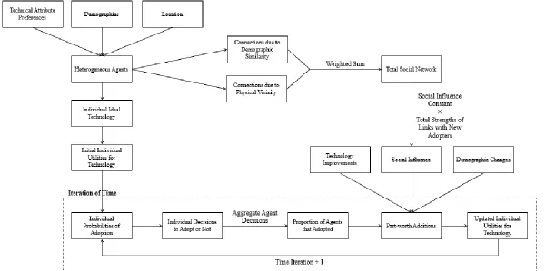
3.3 Agent-Based Model Development

The agent-based model (Figure 3.1) explicitly represents technical and dynamic nontechnical

attributes. A group of agents is created that have demographics, preferences for technical

attributes of a technology, a known location, and are a part of a social network. For each time

step of the simulation, an agent’s observed utility for the technology introduced into the

market is calculated. Then, the binary logit model probability of adoption (Equation (2.6)) is

used to determine each agent’s probability of adoption. If the probability of adoption

surpasses 50%, the agent is considered to have adopted a system. The percentage of agents

who has adopted is recorded after each time step. This process is repeated 30 times to

Agent demographics

Demographic information can be collected using surveys or can be taken from existing

information. In this work, demographic information is taken from the free online version of

the GIS (geographic information systems) company Esri’s tool, Tapestry [64], which

provides data on average age, average annual income, demographic group descriptors, and

more for US ZIP codes. For individual agents, values for each demographic are pulled from a

normal distribution with means based on these averages and standard deviations

representative of the market.

Technical attribute preferences

Preferences for technical attributes can be estimated by collecting responses to CBC surveys

and using a discrete choice model to estimate part-worths for each technical attribute level.

Without information from surveys, the preferences in this research are generated by

considering: 1) a review of literature to determine the relative importance of each technical

attribute when making purchase decisions for a technology [40,65], 2) using the same order

of magnitude as the outside good option (one), and 3) sorting each agent into a group that

represents how early in the adoption curve the agent is likely to purchase a technology.

Four groups were used based on the work of Moore [66]: “early early” adopters, technology

enthusiasts that are the first to try a technology (5%), early adopters (10%), those who are

hesitant to be the first but adopt before the majority of the market, majority adopters (70%),

levels was assigned (see Appendix C to see all standard utilities), with the “early early”

adopter class’s part-worths being the highest, translating to a higher probability of adoption,

and the late adopter class’s part-worths being the lowest. Technical attribute part-worths for

individual respondents were then pulled from a normal distribution with means

corresponding to these mean part-worths and a standard deviation of 0.25. This standard

deviation was chosen so that there was enough part-worth variation to represent

heterogeneous behavior. The value at which this occurred was found by observing the

adoption forecasts resulting from various standard deviations and selecting the value at which

discrete adoptions occurred.

Constraints were applied to the part-worth values to ensure that preference structures

exhibited a smaller-is-better or a larger-is-better structure, as appropriate. As an example,

consider an attribute that reflects the fuel efficiency of a vehicle. Constraints are often used in

model estimation to ensure that the part-worth is smaller for 10 MPG than 20 MPG. These

constraints are applied by assigning the larger of two values as an attribute level’s part-worth:

the part-worth value pulled from a normal distribution and the part-worth value for the worse

attribute level.

Nontechnical attribute part-worth additions

The observed utility for a technology can be estimated using consumer choice models

discussed in Section 2.3, where the observed utility for a technology estimated using a binary

logit model and responses to a CBC survey has the mathematical form of Equation (2.4),

𝑉_𝑛𝑗 = ∑ ∑ 𝛽_𝑛𝑘𝑙𝑥_𝑗𝑘𝑙

𝐿

𝑙=1 𝐾

𝑘=1

(3.2)

However, a consumer’s observed utility for a technology changes over time as a result of

nontechnical attributes. Part-worth additions to the observed utility of the technology each

time iteration represent agents’ increase in value for the technology relative to its

alternatives. The nontechnical attributes considered in this research are social influence,

demographic changes over time, and technology improvements over time. The part-worths

representative of demographic changes and technology improvements, such as changes in

income, increasing age of the adopter, and decreases in price of the technology, are assumed

to only increase over time (as is appropriate according to historical data trends). Each

part-worth representative of influence from another agent is also considered to have a positive

effect on the probability of adoption. Equation (3.3) shows how the part-worth additions

affect agents’ observed utility of the system put to market.

𝑉_𝑛𝑗(𝑡) = ∑ ∑ 𝛽_𝑛𝑘𝑙𝑥_𝑗𝑘𝑙

𝐿

𝑙=1 𝐾

𝑘=1

+ 𝛽_𝑆𝐼𝑥_{𝑆𝐼,𝑛}(𝑡) + 𝛽_𝐷𝐶𝑥_{𝐷𝐶,𝑛}(𝑡) + 𝛽_𝑇𝐼𝑥_{𝑇𝐼,𝑛}(𝑡) (3.3)

The variables in Equation (3.3) are as follows:

 𝛽𝑛𝑘𝑙 and 𝑥𝑗𝑘𝑙: consumer 𝑛’s part-worth and corresponding active attribute level

indicator variable for alternative 𝑗’s 𝑘 technical attributes and corresponding 𝑘𝑙 levels

 𝛽_𝑆𝐼 and 𝑥_{𝑆𝐼,𝑛}(𝑡): part-worth and consumer 𝑛’s time iteration-dependent active

attribute indicator variable representative of the effects of social influence

 𝛽_𝐷𝐶 and 𝑥_{𝐷𝐶,𝑛}(𝑡): part-worth and consumer 𝑛’s time iteration-dependent active

attribute indicator variable representative of the effects of demographic changes

 𝛽_{𝑇𝐶,𝑛} and 𝑥_{𝑇𝐶,𝑛}(𝑡): part-worth and consumer 𝑛’s time iteration-dependent active

attribute indicator variable representative of the effects of technology improvements

The active attribute indicator variable for demographic changes is increased by a constant

each iteration of time (each representing 6 months). The order of magnitude and value of

each demographic change’s corresponding part-worth is chosen so that the part-worth

additions increase initial adoption over time in a manner similar to the historical adoption

trends. The value of the part-worths are also rooted in data; for example, the increase in cost

for a product alternative can be projected forward based on past patterns in cost increase. In

addition to all part-worths being on the same order of magnitude, the part-worth additions for

each demographic change and technology improvement are chosen so that they represent that

attribute’s magnitude of effect on adoption relative to the other attributes. For example, the

part-worth addition for the demographic attribute income is going to have more of an effect

on adoption for a high-cost technology than would the demographic attribute age.

The process of constructing the demographic similarity component of the social network was

presented in Section 2.4, as it is built upon the work of He et al. [11]. This section will

present the methodology for constructing the physical vicinity component of the social

network.

Connections between agents due to physical vicinity were generated to determine the

probability of a connection to a neighbor. A random number generator was then used to

define the presence or absence of a weak or strong connection. Since the effects of nearby

installations are localized, the probability of having a connection with someone in the

consumer’s immediate area is assumed to be twice as high as the probability of having a

connection with a consumer geographically nearby.

The parameters used to define probabilities of connections are the average number of

connections that each node (potential adopter) has, 𝑐̅, and the percentage of these connections that are strong, 𝑝_𝑠. Equations (3.4) and (3.5) were used to find the total probabilities of having a strong and weak connection with someone else in the social network, respectively,

based on these two social network parameters.

𝑃(𝑆) =𝑐̅ ∙ 𝑝𝑆

𝑁 (3.4)

𝑃(𝑊) =𝑐̅ ∙ (1 − 𝑝𝑆)

where 𝑁 is the total number of consumers in the social network. These probabilities are used to determine the:

 probability of a strong connection with another consumer in their immediate area,

 probability of a weak connection with another consumer in their immediate area,

 probability of a strong connection with another consumer somewhat nearby,

 and, the probability of a weak connection with another consumer somewhat nearby

A random number generator is used to decide the presence of a weak and strong connection

between each pair of agents in the network. The indicator variable 𝐿_{𝑃𝑉𝑛1𝑛2} is defined similar to the indicator connection for demographic similarity where 𝐿_{𝑃𝑉𝑛1𝑛2}is equal to 2 when a strong connection is present, 1 when a weak connection is present, and 0 when no connection

is present.

The two components of the social network (demographic similarity and physical vicinity) are

then combined via a weighted sum:

𝐿_{𝑇𝑂𝑇𝑛1𝑛2} = 𝑤₁𝐿_{𝐷𝑆𝑛1𝑛2}+ 𝑤₂𝐿_{𝑃𝑉𝑛1𝑛2} (3.6)

Accounting for social influence as a result of the constructed social network

Once the total social network has been created using Equation (3.6), the Watts-Strogatz

mechanism [60] is used to turn the existing social network into a small-world network by

introducing a probability 𝛼 that each connection between a specific node and all of its connections will be “rewired” to another random node (in this work, the rewiring probability

is set to 𝛼 = 0.1 as in the work of He et al. [11] and other existing literature [61–63]). The small-world network was introduced by Watts-Strogatz in 1998 [60] and has been shown to

represent empirical networks including social networks (based on the small-world

phenomenon or “six degrees of separation” as it is commonly referred to) [61–63]. The

small-world network is classified by short average path length and a high clustering

coefficient, where average path length is the average distance between two nodes within the

network and the clustering coefficient is the probability that two randomly selected

connections of a node in the network will also be connected.

Any time an agent adopts the technology the other agents that agent is connected to has their

utility for the technology increased by a part-worth addition. The magnitude of the part-worth

addition is found by multiplying a constant by the total strengths of the connections with new

adopters. For example, consider agent 𝑥 who has a connection to agents 𝑦 and 𝑧. Consider that these agents both just adopted the technology and have connection strengths of 2 and 3,

depicts how the part-worth addition representing social influence is calculated for agent 𝑖 where 𝑁 is the total number of agents in the social network.

𝛽_𝑆𝐼𝑥_{𝑆𝐼,𝑛𝑖}(𝑡) = 𝛽𝑆𝐼∙ ∑ 𝐿𝑇𝑂𝑇_{𝑛𝑖𝑛𝑗}(𝑡) 𝑁

𝑗=1

CHAPTER 4 – SIMULATION OF ROOFTOP RESIDENTIAL SOLAR SYSTEM ADOPTION IN CARY, NC

4.1 Motivation

Residential rooftop solar systems continue to be one of the most commonly installed forms of

residential distributed generation of electricity [28]. A 2012 study by Hart Research showed

that more respondents think it is either very or somewhat important to develop and use solar

photovoltaics (PV) in the US [67]. Though the concept of converting solar energy into

electricity has been around for over 150 years, solar PV did not achieve an efficiency great

enough for commercial use until the mid-1950s [68]. However, residential solar systems did

not see widespread usage in the US until 2007, when California followed the examples of

Germany and Japan to subsidize the use of residential solar systems [69]. This work develops

an agent-based adoption model using the characteristics of a group of neighborhoods in Cary,

NC and the technology of residential solar systems.

4.2 Selection of Simulation Neighborhoods

A group of four neighborhoods in Cary, NC that share borders was selected based on ZIP

code characteristics found using the free online version of the GIS (geographic information

systems) company Esri’s tool, Tapestry [64]. Information on these neighborhoods can be

found in Appendix A. The characteristics of the residents living in multiple North Carolina

ZIP codes were compared to the profile of likely residential solar system adopters as found

by studies such as [70]: a household annual income between $85,000 and $115,000, age of

ZIP code near the researchers (Raleigh, NC) and looking for these qualities, the ZIP code

27518 representing a percentage of Cary, NC was selected. Tapestry shows that the ZIP code

27518 has an average annual income of $110,000, a mean resident age of 41.5, and high

levels of higher education degrees.

Instead of assuming that all of the homes in the neighborhood should be included in the

social network, and therefore influence the adoption forecast models, the homes that could

not support a residential solar system were eliminated from the study. Suitability is

determined using the sunlight hours, roof space, and 20 year savings gained from installing a

residential solar system reported by Google’s tool Project Sunroof [71]. If installing a

residential solar system affords the homeowner no savings over 20 years, it is assumed that

the homeowner will not invest in system.

4.3 Selection of Technical Attributes and Levels

The first step in the development of the agent-based model was the selection of the technical

attributes and levels to represent the residential solar systems. In any CBC survey, the

number of technical attributes included has to remain low enough so that the survey taker is

not overwhelmed but large enough to accurately represent the technology. After reviewing

works that summarize the most important considerations of homeowners when they are

deciding to adopt a residential solar system [40,70,72], the list was narrowed to:

 monthly cost savings on the homeowner’s observed utility bill in percent,

 payback period in years,

 production warranty in years, and

 price per kilowatt of the system in dollars.

The attributes and the selected levels for each are displayed in Table 4.1. The reasoning

behind the selection of these levels is given in this section.

Table 4.1: Attributes and levels chosen to represent residential solar systems

Attribute Level 1 Level 2 Level 3 Level 4

Monthly Cost Savings ≤ 25% >25%, ≤ 50% >50%, ≤75% > 75%

Payback Period 5 years 10 years 15 years 20 years

Financial Incentive Structure

$0.02/kWh produced

$1.05/W installed up to $10,000

30% tax credit

Production Warranty 10 years 15 years 20 years

Purchase Price $1,500/kW $2,250/kW $3,000/kW

Monthly cost savings

Monthly cost savings refers to the percentage of the resident’s monthly utility bill that the

residential solar system covers by producing power that the residents would have otherwise

had to purchase from the traditional grid. Cost savings are dependent on both the size of the

system installed and the power consumption of the household. The attribute levels selected

for this attribute represent all possible values within this attribute.

Payback periods of residential solar systems can reach up to 20 years. The attribute levels

selected for payback period are representative of typical payback periods. Typical payback

periods were calculated based on a review of existing financial incentive structures

nationwide [73] and average residential solar system upfront costs for multiple system sizes.

An analysis of payback periods for these multiple system sizes (which can be found in

Appendix D) showed a range of payback periods from 3 to 20+ years, with the vast majority

of payback periods falling between 5 and 15 years.

Financial incentives

Financial incentives [65,72] include multiple federal, state, and local government programs

that promote the installation of residential solar systems, most of which are listed Database of

State Incentives for Renewables & Efficiency (DSIRE) Solar [73]. The structures that

financial incentives can take include rebates, loans, grants, feed-in tariffs, tax credits, and tax

deductions. After compiling a list of the financial incentives available nationwide applicable

to residential solar PV technology, the most common financial incentive structures were

found to be feed-in tariffs, rebates, and tax credits. Corresponding attribute levels were

defined for each of these structures.

Warranty

The terms of a production warranty vary across different companies, but in general it is the

number of years that either the manufacturer or installer guarantees the rated production from