An Analytical and Numerical Study of a Class of Nonlinear Evolutionary PDEs.

(1)

ABSTRACT

PENDLETON, TERRANCE LAMAR. An Analytical and Numerical Study of a Class of Nonlinear Evolutionary PDEs. (Under the direction of Dr. Alina Chertock.)

This thesis concerns itself with an analytical and numerical study of a family of evolutionary partial differential equations (PDEs) which supports peakon solutions for special values of a given bifurcation parameter. Here, the bifurcation parameter describes the balance between convection and stretching for small viscosity in the dynamics of one dimensional (1D) nonlinear waves in fluids.The first portion of this thesis is to provide global existence and uniqueness results for the considered family of evolutionary PDEs by establishing convergence results for the particle method applied to these equations. This particular class of PDEs is a collection of strongly nonlinear equations which yield traveling wave solutions and can be used to model a variety of flows in fluid dynamics. We apply a particle method to the studied evolutionary equations and provide a new self-contained method for proving its convergence. The latter is accomplished by using the concept of space-time bounded variation and the associated compactness properties. From this result, we prove the existence of a unique global weak solution in some special cases and obtain stronger regularity properties of the solution than previously established. The second portion of this thesis is dedicated to studying the dynamics of the in-teraction among a special class of solutions of the one-dimensional Camassa-Holm (CH) equation which are a particular example of such a PDE which supports peakon solutions. The equation yields soliton solutions whose identity is preserved through nonlinear in-teractions. These solutions are characterized by a discontinuity at the peak in the wave shape and are thus called peakon solutions. We apply a particle method to the CH equa-tion and show that the nonlinear interacequa-tion among the peakon soluequa-tions resembles an elastic collision, i.e., the total energy and momentum of the system before the peakon interaction is equal to the total energy and momentum of the system after the collision. From this result, we provide several numerical illustrations which supports the analytical study, as well as showcase the merits of using a particle method to simulate solutions to the CH equation under a wide class of initial data.

(2)

(3)

(4)

An Analytical and Numerical Study of a Class of Nonlinear Evolutionary PDEs

by

Terrance Lamar Pendleton

A dissertation submitted to the Graduate Faculty of North Carolina State University

in partial fulfillment of the requirements for the Degree of

Doctor of Philosophy

Applied Mathematics

Raleigh, North Carolina 2013

APPROVED BY:

Dr. Michael Shearer Dr. Mark Hoefer

Dr. Pierre Gremaud Dr. Alina Chertock

(5)

DEDICATION

In memory of my father, Howard L. Pendleton who gave me opportunities he never had. To my mother, my family and my friends for making sure that I did not lose my mind

(6)

BIOGRAPHY

(7)

ACKNOWLEDGEMENTS

It is difficult to find the right combination of a finite number of words to express my gratitude for my advisor, Dr. Alina Chertock. I am eternally grateful for the knowledge, mentoring, care, and patience she bestowed on me. Without her assistance, this endeavor would remain but a dream. I am equally grateful for the contagious love for PDEs that she help instilled in me. I look forward to spreading the same joy and love for this subject to others.

Many other professors and advisors have helped paved the way to obtaining my goal here at NC State. I am thankful for having such a supportive group of members on my thesis committee. With kind words, and constructive feedback, Dr. Mark Hoefer, Dr. Pierre Gremaud, and Dr. Michael Shearer have helped better me as a graduate student, and for this I am forever grateful. Special thanks also goes to professors Dr. Robert Martin and Dr. Sandra Paur for teaching me the tools for not only surviving graduate school but flourishing.

To my parents Howard and Phyllis who have invested so much into me. At every step of the way, they were with me even though they were physically hundred of miles away. Since the instant I was born, they loved and cared for me in a way that I can never fully understand. It is an honor to be their son and to carry their name.

While there can never be a comprehensive list of all of the people on this earth who made this degree a reality, I feel obligated to mention the name of a few friends whose support and guidance meant beyond what they realize. To Kaska Adoteye, George Lankford, Daisy Sudparid, Cre’Shannon Thompson, Karmethia Thompson, Cleveland Waddell, Nakeya Williams, thank you for your friendship. You have offered motivational words and support when I have needed it most and you have helped keep me grounded and in check when appropriate. You have been willing to listen and offer advice when needed, and even laugh at my never ending flow of corny jokes.

(8)

LIST OF FIGURES

Figure 3.1 Two positive peakon interaction for the CH equation(3.1) for various times.. . . 59 Figure 3.2 Location and momentum trajectories for the two positive peakon

in-teraction. . . 59 Figure 3.3 The velocity u for the CH equation(3.1) at t=1, and the associated

particle location trajectories. . . 60 Figure 3.4 The velocity u for the CH equation(3.1) at t=2, and the associated

particle location trajectories. . . 61 Figure 3.5 The velocity u for the CH equation(3.1) at t=8, and the associated

particle location trajectories. . . 61 Figure 3.6 The velocityufor the CH equation(3.1) att=10, and the associated

particle location trajectories. . . 61 Figure 3.7 An Illustration of the peakon-antipeakon phenomenon at various times. 63 Figure 3.8 Location and momentum trajectories for the peakon-antipeakon

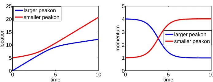
in-teraction. . . 63 Figure 3.9 (Zoomed) Location trajectories for the peakon-antipeakon interaction. 64 Figure 3.10 An Illustration of the peakon-antipeakon (with different magnitudes)

phenomenon at various times. . . 65 Figure 3.11 Location and momentum trajectories for the peakon-antipeakon (with

different magnitudes) interaction. . . 65 Figure 3.12 (Zoomed) Location trajectories for the peakon-antipeakon (with

dif-ferent magnitudes) interaction. . . 66 Figure 3.13 The velocity u obtained by both PM and FV at times t= 1,10 with

Np =Nc= 500. . . 69

Figure 3.14 The velocity u obtained by both PM and FV at times t = 1 with

Np = 500, Nc= 3000. . . 70

Figure 3.15 The velocityufor the CH equation obtained by FV and PM at various times with Np =Nc= 500. . . 71

Figure 3.16 The velocityu for the CH equation at t=9 with Np = 500, Nc= 3000. 71

Figure 3.17 The velocityufor the CH equation obtained by FV and PM at various times with Nc=Np = 500. . . 73

Figure 3.18 Grid refinement analysis for both FV and PM att= 10. . . 74 Figure 3.19 The velocityufor the CH equation obtained by FV and PM att= 10,

Nc= 7000 and Np = 500. . . 74

Figure 4.1 The velocity u and density ρ for the 2CH equation at various times with ∆x= 0.029 using the CU scheme. . . 88 Figure 4.2 The densityρ for the 2CH equation obtained by at various times with

(11)

Figure 4.3 The densityρ for the 2CH equation obtained by at various times with

∆x= 0.029, α= 0.05 using the CU scheme. . . 89 Figure 4.4 The velocityu for the 2CH equation obtained at timet = 0.02using

(12)

Chapter 1

Introduction

This thesis concerns itself with an analytical and numerical study of a family of evolu-tionary partial differential equations (PDEs) which supports a special class of solitary traveling waves for special values of a given bifurcation parameter (b). To this extent, we are are interested in studying

mt+mxu+bmux = 0 u=G∗m, x∈R, t >0, (1.1) with the parameter b ∈_Rand is considered subject to the initial condition

m(x,0) =m0(x) x∈R. (1.2)

Here the momentum m and velocity u are functions of the time variable t and the spatial variablex, andG(x) is the Green’s kernel which relatesmwithuthrough a convo-lution. The parameter b describes the balance between convection (mxu) and stretching

(bmux) for small viscosity in the dynamics of one-dimensional (1-D) nonlinear waves in

fluids. In other words, the real dimensionless constant b is the ratio of stretching to con-vection transport. b can also be seen as the number of covariant dimensions associated with the momentum density m as was shown in [80] and provides a balance for the non-linear solution behavior. We remark that for the remainder of this thesis, we will focus our efforts on (1.1) with b >1 which generates stable solitary traveling waves.

(13)

developed in this thesis. We also provide an outline for the remainder of the thesis. An important research area in the field of PDEs involves the study and establishment of global solutions for a variety of equations. The equations given by (1.1) (b-equations) are a family of first-order hyperbolic problems and have been studied in a variety of contexts. Moreover, they have been shown to possess several interesting properties. For instance, the b-equations’ invariance under space and time translations ensures that it admits traveling wave solutions for b > 1 (although this is true for any b ∈ _R). In particular, the traveling wave solutions assume the formu(x, t) =aG(x−ct), with speed c = −aG(0), which is proportional to the solution amplitude and G is the kernel in (1.1). The kernelG(x) relates the velocity with the momentum through the convolution product

u=G∗m =

Z

R

G(x−y)m(y, t)dy, (1.3)

and determines the shape of the traveling wave and the length scale for (1.1); see e.g., [81].

The derivation of traveling wave solutions associated with (1.1) can be found in [80] where

u=u(z) and m =m(z), where z =x−ct, (1.4) and c is the wave speed. In what follows, we will let 0 denote d/dz and rewrite (1.1) in the form of the conservation law

m1/b_t+ m1/bu_x = 0. (1.5)

Forb 6= 0, the conservation law (1.5) for traveling waves becomes

(u−c)m1/b0 = 0, (1.6)

which after integrating gives

(u−c)bm=K. (1.7)

Forb >0, (1.1) has nontrivial solutions (m(x, t)) vanishing as|z| → ∞so that K = 0 in (1.7). Thus, one obtains

(14)

which yields the generalized function solutions

m=cδ(z) and u=G∗m =cG(z),

matched by u−c= 0 at z = 0 and where δ(x) is the Dirac delta-function. This gives a traveling wave, whose shape in uis given by the kernel G. Nonlinear interactions among these solutions are governed by the following superposition of solutions:

u(x, t) =

N

X

i=1

pi(t)G(x−qi(t)). (1.9)

This class of solutions satisfy a finite dimensional dynamical system for the amplitudes denoted by pi(t), and the associated locations denoted by qi(t).

The family of evolutionary PDEs given by (1.1)–(1.2) arises in diverse scientific appli-cations such as shallow water waves, computational anatomy, mechanical vibrations and turbulent fluid flows (see, e.g. [20, 73, 76, 77, 78]). These equations also enjoys several remarkable properties both in the 1-D and multi-dimensional cases, see, e.g. [16, 110]. The quadratic terms in (1.1) represents the balance in fluid convection between nonlinear transport and amplification due to b-dimensional stretching. If one considers G as the Green’s function associated with the modified 1-D Helmholtz operator, I−α2_∂

xx, then

G(x) = 1 2αe

−|x|/α_, _(1.10)

and (1.1) reduces to

mt+mxu+bmux = 0 m=u−α2uxx, x∈R, t >0, (1.11)

where α is some length scale. If, for example, we consider m as the fluid momentum in (1.11) then we have b = 2; see e.g., [81]. It turns out that this case b = 2 coincides with the dispersionless case of the Camassa-Holm (CH) equation for shallow water waves. Furthermore, the case for b = 3 coincides with the Degasperis-Procesi (DP) equation used to model the propagation of nonlinear dispersive waves, see [55].In this special case, the corresponding traveling wave solutions assume the form u(x, t) = ae−|x−ct|/α_,

with speed c, amplitude a and length α. The traveling wave solutions to (1.11) are characterized by a discontinuity in the first derivative at their peaks since ux(x, t) = −a

αsgn(x−ct)e

(15)

equations are completely integrable as Hamiltonian systems and their peakon solutions are true solitary waves that emerge from the initial data. Peakons for eitherb= 2 orb = 3 exhibit a remarkable stability–their identity is preserved through nonlinear interactions, see, e.g. [16, 129] and [53, 54, 55, 110, 117]. Peakons corresponding to b = 2 and b = 3 are also orbitally stable–i.e. their shape is maintained under small perturbations, see, e.g. [47, 58, 103]. We note that peakons can also be considered as waves of largest amplitude that are exact solutions of the governing equations for irrotational water waves, see [140]. For a more complete discussion on the hydrodynamical properties of peakons generated from the CH or DP equation, we refer the reader to [45, 86].

The two-dimensional (2-D) version of (1.11) withb = 2, the so-called EPDiff equation (Euler-Poincar´e equation associated with the diffeomorphism group) is given by

∂m

∂t +u· ∇m+∇u

T_·_m₊_m(div_{u) = 0,} _m₌_u₋_α2_∆u, _(1.12)

and appears in the theory of fully nonlinear shallow water waves [78, 79, 80, 81]. Applying viscosity to the incompressible, three-dimensional analog of this equation produces the Navier-Stokes α-model for the averaged fluid equations (see, e.g., [20]). The equation (1.1) has many further interpretations beyond fluid applications. For instance, in 2D, it coincides with the averaged template matching equation (ATME) for computer vision (see, e.g., [73, 76, 77]). One could also use (1.1) to quantify growth and other changes in shape, such as occurs in a beating heart, by providing the transformative mathematical path between the two shapes, (see, e.g, [78]).

The Cauchy problems for both the CH (b= 2) and DP (b = 3) equations have been extensively studied in the literature. We refer the reader to a review paper [121], where a survey of recent results on well-posedness and existence of local and global weak solutions for the CH equation is presented. In particular, the local well-posedeness results for the CH equation in Hs(_R), s > 3/2, were established in [40, 108, 133]. The continuation of solutions to the CH equation after wave breaking in L∞(_R+, H1(R)) was established in

[11, 12]. The existence of a global weak solution to the CH equation in L∞(_R+, H1(R)) was proven in [11, 41, 145] and in [46], it was shown that this global solution is unique.

Recent results related to well-posedness and existence of local and global weak solu-tions of the DP equation can be found, e.g., in [37, 60, 116, 147, 148], where it was proven that the global weak solutions of the DP equation belong to L∞(_R+, H1(R)) and global

(16)

local well-posedeness and several global existence results were obtained in [61] for a gen-eral case of the initial-value problem (IVP) (1.11), (1.2) with different values of the parameter b.

Capturing peakon solutions numerically poses quite a challenge–especially if one con-siders a peakon-antipeakon (a peakon with negative initial weight) interaction. Several nu-merical methods have been proposed for simulating peakon interactions for the CH equa-tion such as finite-difference [38, 74, 75], finite-volume [3] finite-element [119, 132, 146], and spectral [34, 39, 62, 88, 89] methods. A few numerical methods, such as conservative finite-difference schemes, have been used to study the DP equation (see [118]). Many of these methods are computationally intensive and require very fine grids along with adaptivity techniques in order to simulate the peakon behavior.

Solutions of (1.1), (1.2) can be accurately captured by using a particle method as it was shown in our paper [31] as well as in [17, 18, 22] for the CH equation and in [22] for the EPDiff equation. In the particle method, described in our paper [31] and in [22], the solution is sought as a linear combination of Dirac distributions, whose positions and coefficients represent locations and weights of the particles, respectively. The solution is then found by following the time evolution of the locations and the weights of these particles according to a system of ODEs obtained by considering a weak formulation of the problem. The particle methods presented in [17, 18] have been derived using a discretization of a variational principle and provide the equivalent representation of the ODE particle system. The main advantage of particle methods is their (extremely) low numerical diffusion that allows one to capture a variety of nonlinear waves with high resolution, see, e.g., [25, 29, 30, 131] and references therein.

A convergence analysis for the particle method applied to the CH equation was studied in [129] and in our paper [31]. In [129], the authors used the Hamiltonian structure of the CH equation and its complete integrability to establish error estimates for the particle method when the solutions are smooth. In our paper [31], the convergence of the particle method for the CH equation has been proven using the concept of space-time bounded variation. Properties of the particle method were also studied in the context of the DP equation in [53, 54, 55, 81].

(17)

Chapter 2, we provide global existence and uniqueness results for the family of fluid transport equations given by (1.1) by establishing convergence results for the particle method applied to these equations. In Chapter 3, we study the dynamics of the interaction among a special class of solutions of the 1-D CH equation as well as showcase the merits of using particle methods to simulate solutions to the CH equation using arbitrary smooth initial data. In Chapter 4, we consider a two-component generalization of the CH equation as a possible model for the long time propagation of tsunami waves by implementing a variety of numerical methods with pertinent initial data. In Chapter 5, we conclude the thesis by providing some future goals related to our study.

1.1

Camassa Holm Equation and Its Generalizations

Completely integrable nonlinear evolutionary partial differential equations often arise in various applications in shallow water wave theory. By completely integrable, we mean that there is some change of variables such that the given evolution equation in the new variables is equivalent to a linear flow at constant speed. The Korteweg-de Vries (KdV) equation is perhaps one of the most famous and extensively studied examples in this particular class of equations (see e.g. [90]). The KdV equation is typically regarded as the prototypical example of a nonlinear evolutionary PDE whose solutions can be exactly specified and are given by solitons– localized solutions which undergo a strongly nonlinear complex interaction but retain their form after the interaction, with the possible exception of a phase shift [102]. This thesis concerns itself with the CH equation (and one of its generalizations) which describes surface waves in shallow water.

In 1993, Roberto Camassa and Darryl Holm proposed a new completely integrable dispersive shallow water equation by using an asymptotic expansion directly in the Hamil-tonian for Euler’s equations in the shallow water regime [129]:

mt+umx+ 2uxm =−c0ux−γuxxx, m =u−α2uxx. (1.13)

Herem=u−α2_u

xx is the momentum variable,α2 and γ/c0 are squares of length scales,

and c0 = √

g0_h _{is the linear wave speed for undisturbed water of depth} _h _{at rest under}

gravityg0 at infinity. We note that any constant valueu=u0 is also a solution of (1.13).

With an appropriate Galilean transformation and a velocity shift (t → t+t0, x →

(18)

as seen in [80]. In this scenario, we are left with the followingdispersionless CH equation: mt+umx+ 2uxm = 0, m =u−α2uxx. (1.14)

Indeed, one can derive a dispersion relation for (1.1) to understand why (1.1) corre-sponds to the dispersionless CH equation (for the caseb = 2). To this extent, we assume a plane wave solution for the momentum m of the form:

m(x, t) = m0+Aei(kx−ωt) =m0+v(x, t). (1.15)

Here,m0 is the background uniform momentum,kis the wave number,|A| 1 is a small

complex parameter (necessary for the linearizion) andω is the frequency. By a dispersion relation, we seek a relationship between k and ω of the form

ω =ω(k). (1.16)

We calculateu from (1.3) and (1.15) to obtain

u=G∗(m0+v(x, t))

=G∗m0+G∗v(x, t)

=m0

Z ∞

−∞

G(x−y)dy+Ae−iωt

Z ∞

−∞

G(x−y)eikydy

=m0

Z ∞

−∞

G(x−y)dy+Aeikx−iωt

Z ∞

−∞

G(z)e−ikzdz

=m0F[G](0) +F[G](k)v,

(1.17)

where F[G](k) is the Fourier transform of G(x) and is given by

F[G](k) =

Z ∞

−∞

G(x)e−ikxdx. (1.18)

We substitute (1.15) and (1.17) into (1.1) to obtain

(19)

To derive a dispersion relation, we linearize (1.19) to obtain

vt+ (m0F[G](0) +bm0F[G](k))vx = 0. (1.20)

Usingv as was given in (1.15) to calculate vt and vx, we obtain the following dispersion

relation

ω(k) = km0(F[G](0) +bF[G](k)). (1.21)

Assuming that b 6= 0, from (1.21), we see that if m0 = 0, then the linearized flow is

dispersionless (i.e. w00(k) = 0). This is what is meant by thedispersionless CH equation. We recall that traveling waves, associated with differential equations, are solutions of the form

u(x, t) = f(x−ct), (1.22)

which represents waves of a permanent shape f that propagates at some constant speed c. The waves given by (1.22) aresolitary if they are localized in the sense that the wave profile decays at infinity. If in addition, these solitary waves retain their shape and speed after interacting with other waves of the same type, then these waves are referred to as solitons. The traveling wave solutions to (1.14) are given by (1.22) with f(x) = 1

2αe

−|x|/α

and are hence referred to as peakons–solitons with a sharp peak that is characterized by a discontinuity in the first derivative. We remark that these particular traveling wave solutions may be easily deduced by taking G(x) as given in (1.10). The interactions among N peakons are given by

u(x, t) = 1 2α

N

X

i=1

pi(t)e−|x−qi(t)|/α, (1.23)

where the amplitudespi(t) and the locations qi(t) are given by a 2N dimensional

dynam-ical system (c.f. [129]) to be determined by substituting (1.23) into (1.14). This forms the basis for applying a particle method for numerically simulating solutions to the considered equations. We further discuss the particle method in the sections that follow.

(20)

from the knowledge of a smooth initial profile it is possible to predict the occurrence of wave breaking. If wave breaking occurs, then one can proceed with the continuation of solutions in one of two ways. One may consider either the conservative case which is characterized by the conservation of energy or the dissipative case which accounts for the the loss of energy due to breaking.

In [129], Camassa and Holm first observed that (1.13) was bi-Hamiltonian; that is, the equation can be expressed in Hamiltonian form in two different ways. Recalling that m = u−α2uxx, the two compatible Hamiltonian descriptions of the CH equations are

given by

mt =−(m∂x+∂xm)

δH1

δm =−∂x 1−α

2_∂2 x

δH2

δm =−∂x δH2

δu , (1.24) with the following conserved quantities:

H1 =

1 2

Z

R

u2+α2u2_x dx and H2 =

1 2

Z

R

u3+α2uu2_x dx.

Because of this unique property, the CH equation possesses an infinite number of conser-vation laws. Given the fact that both the KdV equation and the CH equation are com-pletely integrable, it is no surprise that the KdV equation and CH equation are related in some formal way. Indeed, the KdV equation appears at linear order in an asymptotic expansion for unidirectional shallow water waves in a free surface under gravity. The ex-pansion is made in terms of two small dimensionless ratios for small-amplitude long waves in shallow water. At quadratic order in the same asymptotic expansion, the Camassa-Holm equation is derived. We note that the KdV equation may be recovered if we take α2 →0. Additional information regarding the derivation and associated properties of the CH equation may be found in [43, 44, 51].

(21)

mt+umx+ 2mux =−gρρx,

ρt+ (ρu)x = 0.

(1.25)

Similar to the CH equation, one may derive a dispersion relation for (1.25). To this extent, we assume a plane wave solution for the momentum m and the density ρ of the forms:

m(x, t) =m0+Aei(kx−ωt)=m0+v(x, t),

ρ(x, t) = ρ0+Bei(kx−ωt) =ρ0+w(x, t).

(1.26)

Here, m0 is the background uniform momentum, ρ0 is the background uniform density,

k is the wave number, |A|,|B| 1 are small complex parameters (necessary for the linearizion) and ω is the frequency. By substituting (1.26) and (1.17) into (1.25) and linearizing the results we obtain

vt+ (m0F[G](0) + 2m0F[G](k))vx =−gρ0wx,

ρt+ρ0F[G](k)vx+m0F[G](0)wx = 0.

(1.27)

Using our definition for v and w in (1.26), we obtain the following system of equations written in matrix form

 

−ω+km0(F[G](0) + 2F[G](k)) kgρ0

kρ0F[G](k) −ω+m0kF[G](0)

 

 

A

B

 =

 

0 0

 

Since A, B 6= 0, we must have that det(M) = 0 where

M =

 

−ω+km0(F[G](0) + 2F[G](k)) kgρ0

kρ0F[G](k) −ω+m0kF[G](0)

 .

Thus, to find the dispersion relation, we must solve

(−ω+km0(F[G](0) + 2F[G](k))) (−ω+m0kF[G](0))−gk2ρ20F[G](k) = 0, (1.28)

for ω. Solving this quadratic equation for ω yields the following results:

ω(k) =m0kF[G](0) +m0kF[G](k)±

q

m2

(22)

This particular multicomponent generalization of the CH equation has been studied extensively and was shown to be completely integrable in [42]. Additionally in [42], it was shown that similar to the CH equation, (1.25) has a Lax pair formulation and is bi-Hamiltonian. Many others studied a modified version of (1.25) which supports peakon solutions (see e.g. [59, 123] and references therein). However, a hallmark feature of (1.25) is that the system was shown to be physically relevant in [42]. There, it was shown how the system given by (1.25) arises in shallow water theory, where it is derived from the Green-Naghdi [69] equations using appropriate expansions in terms of physical pa-rameters. The Green-Naghdi equations themselves are approximate models to the full governing equations [69] and are commonly used in coastal oceanography to describe the propagation of large amplitude surface waves. The shallow water scaling (µ1), gives rise to the Green-Naghdi equations where µ is a dimensionless parameter given by

µ= h

2

λ2,

where h is the mean depth andλ is the typical wavelength of the waves under consider-ation. In [42], it was also shown that the only way for singularities to occur in smooth solutions is through wave breaking–a similar occurrence for the 1-D CH equation. In addition, they were able to establish the global existence of small amplitude solutions of (1.25) and large amplitude traveling wave solutions with initial data that has a sufficient rate of decay. From their investigation, it was determined that unlike the CH equation, the solitary waves generated form (1.25) must be smooth and hence cannot be referred to as peakon solutions. In Chapter 4, we show how the 2CH equation may be derived in the context of shallow water wave theory and from there determine its potential as a relevant model for the long time propagation of tsunami waves.

1.2

Numerical Methods

(23)

con-sider using a finite difference method, for which a function is represented by its values at certain grid points and derivatives are approximated through differences in these values. Another popular numerical tool involves the method of lines, where all but one variable is discretized. The result is a system of ODEs in the remaining continuous variable. One may also consider a finite volume method, where the computational domain is divided into regions or volumes and the change within each volume is computed by considering the flux (flow rate) across the surfaces of the volume. In this thesis, we focus our attention on two particular methods for obtaining a numerical solution for the b-equation of fluid transport equations and its generalizations.

1.2.1

Finite Volume Method For Systems of Conservation Laws

In this section, we describe an important class of numerical methods for solving systems of hyperbolic conservation laws. Finite Volume methods (FV) are typically useful for solving these types of problems thanks to their ability to capture (possibly) discontinuous solutions in an accurate and non-oscillatory manner. To begin the process for formulating a finite volume method for a system of conservation laws, we consider the following (for simplicity) 1-D version of a system of conservation laws:

∂

∂tq(x, t) + ∂

∂xf(q(x, t)) = 0, (1.30)

whereq:= (q1, . . . , qn) andf := (f1, . . . , fn) are mappings fromRn intoRn and (1.30) is

subjected to some initial condition of the form

q(x,0) = q0(x). (1.31)

Here, q(x, t) is the quantity under consideration, f(q) is the flux function, and x and t are the spatial and time variables respectively. If we let A(q) denote the n×n Jacobian of f then we may express (1.30) in the following quasilinear form

(24)

with

A:=

     

∂f1

∂q1 . . .

∂f1

∂qn

..

. . .. ...

∂fn

∂q1 . . .

∂fn

∂qn

     

.

The system given by (1.30) is said to be strictly hyperbolic if its Jacobian matrixA(q) has n real, distinct eigenvalues that can be ordered in such a way: λ1(q)< . . . < λn(q).

In general, if we are given smooth initial conditions and Ais sufficiently smooth, then a smooth solution exists for at least a short time. However, it is well known that for systems of nonlinear conservation laws, a solution may develop a singularity in finite time, even if A and g are infinitely differentiable functions. Thus, while (1.30) is in theconservation form of the conservation law, it is usually advantageous to consider a weak solution to (1.30) in order to study the associated singularities that may arise in the solution. Indeed we say that q(x, t) is a weak/distributional solution to (1.30)–(1.31) if and only if

Z ∞

0

Z ∞

−∞

q(x, t)φt(x, t) +f(q(x, t))φx(x, t)dx dt=−

Z ∞

−∞

q(x,0)φ(x,0)dx, (1.33)

for every C1 _function _φ _{: Ω} _⊂

R×R+ → Rn with compact support. We remark that using integration by parts, one could show that if qand A are C1 _{functions, then (1.33)}

implies that q is a solution to (1.30). We also note that from this definition, we only require q to be locally integrable in _R. To investigate weak solutions for (1.30), we typically solve Riemann problems which are conservation laws of the form (1.30) coupled with the following special class of initial conditions:

qo(x) =

  

ql :x <0

qr :x >0

. (1.34)

(25)

coefficient matrix A(q) = A. For nonlinear problems, the eigenvalues of the Jacobian matrices depend on the solution, and thus the possibility exists that as we evolve the solution, we will observe regions on the wave that propagate faster or slower than other regions. If two characteristics intersect at any given time, then we have a solution that has different values at the same point. That is, the integral surface has folded over on itself. Thus, the solution is discontinuous and we can no longer consider derivatives at this point. To avoid such a situation, we consider the weak form of the PDE (i.e. we look for a solution which satisfies (1.33)). Shocks occur in our solution whenever two characteristic curves carry conflicting information and meet. To investigate the development of shocks in our solution, we let Λ be a surface which separates our considered domain Ω into two separate regions, say Ω1 and Ω2. Suppose that q|Ω1 = q1, and q|Ω2 = q2 are the initial

states in the given regions. Then q satisfies (1.33) if any only if q is a classical solution (i.e q solves (1.30)) in each region Ω1 and Ω2 and the Rankine-Hugoniot (R-H) jump

condition holds along Λ. The R-H jump condition is given by

nt[q] +nx[f(q)] = 0, (1.35)

where the unit normal vector is given by n= (nt, nx). In our example, we have that the

jump across the solution qis given by

[q] =q2−q1, (1.36)

and the jump across the flux function is given by

[f(q)] = f(q2)−f(q1). (1.37)

For additional information regarding hyperbolic PDEs and hyperbolic systems of con-servation laws, we refer the reader to [64, 104, 120, 136, 137, 141]. For more information about the general theory of PDEs, we refer the reader to [64, 83, 120, 128, 138, 142, 149]. We now turn our attention to the formation of finite volume schemes. To this extent, we consider the integral form of a conservation law which takes on the following form:

d dt

Z

Ci

q(x, t)dx=f(q(xi−1/2, t))−f(q(xi+1/2, t)). (1.38)

(26)

Ci =

xi−1/2, xi+1/2

. (1.39)

In the 1-D case, finite volume methods involve dividing a computational domain into subdomains (sometimes called finite volumes and/or grid cells) and then approximating the integral of q(x, t) over these subdomains. We use the fluxes through the endpoints of the intervals to update the approximation at each time step. To this extent, we define our grid cells given in (1.39) by subdividing our computational domain and letting ∆x= xi+1/2−xi−1/2 ,xi =i∆x, and xi+1/2 =xi+ ∆₂x, i= 1, . . . , N, whereN denotes the size

of each subinterval. In each cell average, we denote the approximation of the integral of q(x, t) by ¯q(x, t) given by

¯

qn_i ≈ 1

∆x

Z

Ci

q(x, tn)dx, (1.40)

at time tn _{and ∆x} ₌_x

i+1/2 −xi−1/2. We note that if q(x, t) is a smooth function, then

one may obtain a second-order approximation of the integral given in (1.40) through the midpoint rule. To evolve this cell average in time, we integrate (1.38) from tn _to_tn+1 _to

obtain:

Z

Ci

q(x, tn+1)dx−

Z

Ci

q(x, tn)dx=

Z tn+1

tn

f q(xi−1/2, t)

dt−

Z tn+1

tn

f q(xi+1/2, t)

dt.

(1.41) By rearranging terms and dividing by ∆x we obtain

1 ∆x

Z

Ci

q x, tn+1 dx=

1 ∆x

Z

Ci

q(x, tn)dx− 1

∆x

" Z tn+1

tn

f q(xi+1/2, t)

dt−

Z tn+1

tn

f q(xi−1/2, t)

dt

#

.

(1.42)

(27)

¯

qn_i+1 = ¯qn_i − 1

∆x

" Z tn+1

tn

f q(xi+1/2, t)

dt−

Z tn+1

tn

f q(xi−1/2, t)

dt

#

. (1.43)

We now see that the issue lies in approximating the flux functions. In fact, the decision on how to approximate the integrals in (1.43) is what gives rise to finite volume methods. From (1.43), we see that we are interested in studying numerical schemes of the form

Qn_i+1 =Qn_i − ∆t

∆x F

n

i+1/2−Fin−1/2

, (1.44)

where

F_in₊₁_/₂ ≈ 1

∆t

Z tn+1

tn

f(q(xi+1/2, t))dt. (1.45)

One key advantage in working with grid averages rather then pointwise values for q(x, t) is the ease of mimicking certain useful properties associated with conservation laws. In particular, by considering grid averages, one may ensure that a numerical method is

conservative in the sense that the total mass within the computation domain will be preserved. This is true since the sum PN

i=1Q n

i∆x approximates the integral of q over

the interval [a, b], and thus if our scheme is conservative, then the discrete sum given above will be altered only due to the fluxes at the boundary points. The method that we describe below is an example of a conservation form which is useful for capturing shock solutions.

In choosing how to approximate the fluxes given in (1.45), one should take into account the convergence of the resulting numerical scheme. That is, we require that the numerical solution, generated from applying a finite volume method, should converge to the true solution of the differential equation as the grid is refined (i.e. as ∆x,∆t→0). In analyzing the convergence of a numerical scheme, we are typically concerned with satisfying the following two conditions:

• The finite volume method should beconsistent with the differential equation. That is, the method approximates the solution well locally.

• The finite volume method should bestable. That is, small errors made in each time step do not grow too fast in later time steps.

(28)

approximating the solution. That is, we require that the local truncation error go to 0 as ∆x,∆t →0. We also require that our method be stable. By stable, we mean that small changes in the initial data will result in small changes in the numerical approximation. That is, small errors in each time step should not grow too quickly. To analyze these properties further, we use the hyperbolicity of the equation to write the scheme in a manner that is more convenient for us to study. Since we expect information to propagate in a finite amount of time, one may assume that the fluxes F_in₋₁_/₂ can be obtained by the cell averages on either side of the grid, Qn_i and Qn_i₋₁. With this assumption,the fluxes may be approximated by a function of the form

F_in₋₁_/₂ =F Qn_i, Qn_i₋₁

, (1.46)

whereF is some numerical flux function. This allows us to recast our numerical scheme as

Qn_i+1 =Qn_i − ∆t

∆x F Q

n i, Q

n i+1

−F Qn_i, Qn_i₋₁. (1.47) To determine if a numerical scheme is consistent, we need to check the accuracy of the approximation of the integrals given in (1.45). We observe that ifq(x, t) = ¯q is constant in x, then the integral in (1.45) simply reduces to f(¯q). Thus, if Qn_i₋₁ = Qn_i = ¯q, then the numerical flux function also reduces down to f(¯q), so we require

F(¯q,q) =¯ f(¯q), (1.48)

for any such value ¯q. We also generally expect continuity in F as Qi and Qi−1 vary,

so that F (Qi−1, Qi) → f(¯q) as Qi−1, Qi → q. Thus, we would also like to enforce a¯

Lipschitz continuity condition. That is, we require the existence of a constant L > 0 so that

|F Qn_i, Qn_i₋₁−f(¯q)| ≤Lmax (|Qi−q¯|,|Qi−1−¯q|). (1.49)

(29)

dependence must contain the actual domain of dependence of the PDE. This is obviously necessary, since if there exists information contributing to the evaluation of a quantity that is not being considered by the numerical method, then a change in the initial data outside the numerical domain of dependence would not affect the approximation, while the true solution would change. We remark that the CFL condition is a necessary, but not a sufficient condition for stability. In what follows, we discuss how one may approximate the fluxes to derive a finite volume method for the numerical simulation of systems of conservation laws.

Godunov Schemes

In numerical analysis and computational fluid dynamics, Godunov’s scheme is a conserva-tive numerical scheme, suggested by S. K. Godunov in 1959, for solving partial differential equations. This important class of finite volume methods solves exact, or approximate, Riemann problems at each inter-cell boundary. In its basic form, Godunov’s scheme is first order accurate in both space, and time, yet can be used as a base scheme for devel-oping higher-order methods. In [65], the information available at timetn _{is reconstructed}

using a piecewise polynomial function over the cell averages. To update the information to timetn+1, we must solve a corresponding Riemann problem that results from this re-construction.We remark that the solutions to Riemann problems are not easily accessible nor necessarily available, thus limiting the types of problems to which the method may be applied. For systems of conservation laws, because waves may propagate in different directions, solutions to the Riemann problem are even more complicated. In general, his method can be interpreted as the following REA algorithm:

1. Reconstructa piecewise polynomial function ˜qn(x, tn) from the cell averages Qn_i. In the simplest case, ˜qn_{(x, t}

n+1) is a piecewise constant on each grid cell:

˜

qn(x, tn) =Qn_i, for all x∈Ci.

2. Evolve the hyperbolic equation with this initial data to obtain ˜qn(x, tn+1). 3. Average this function over each grid cell to obtain new cell averages.

Qn_i+1 = 1 ∆x

Z

Ci

˜

(30)

Generally, the piecewise reconstruction is given as:

q(x, tn)≈pn_i(x), for x∈Ci, (1.51)

which is typically discontinuous at the cell interfaces x=xi±1/2.

The stability of the finite volume method is, in general, guaranteed when (1.51) is non-oscillatory, which is accomplished by the use of slope limiters. A library of non-oscillatory reconstructions is available, (see e.g., [1, 36, 64, 71, 72, 91, 97, 106]). A more detailed description of the linear piecewise reconstruction is provided in the section describing the semi-discrete central upwind scheme, which is a special class of FV methods. We note that this piecewise reconstruction allows one to obtain an exact evolution of the solution. This solution is given by a finite set of waves traveling at constant speeds. Typically, depending on the type of grid cells used in the derivation of the scheme, Godunov’s method requires the solutions to the Riemann problems that arise at the grid interfaces. In what follows, we discuss a few possibilities for calculating the numerical flux func-tions in terms of the cell averages available on either side of the flux interface. To this extent, we will consider two ways to determine the control volumes over which the flux function is integrated. These two methods for constructing numerical approximations to the flux functions divide Godunov schemes into two distinct classes: upwind schemes and central schemes.

Upwind Schemes Versus Central Schemes

Recall that for hyperbolic problems, we expect the information to propagate with a finite speed. That is, the waves generated by solving the hyperbolic problem travel at finite speeds. A major goal of upwind methods is to use information about how a solution behaves at previous time steps to determine the numerical flux functions. Upwind meth-ods anticipate the arrival of information along the characteristics on which they travel. Because of this, upwind methods are typically able to produce numerical solutions that are less diffusive.

If we consider the 1-D conservation law given by (1.32), then using upwind schemes, one may update the cell averages att =tn+1 _{by approximating the integrals on the right}

hand side of (1.45). One significant disadvantage involved in using upwind schemes is that since the piecewise polynomial reconstruction is usually discontinuous at the interfaces x=x_j_±1

(31)

As mentioned earlier, this is typically a costly, complicated task. For more information regarding Riemann solvers and upwind schemes, we refer the reader to [5, 9, 36, 64, 65, 91, 104, 141].

Central schemes are usually easier to implement in comparison to upwind schemes, and hence are more applicable to a wide range of problems in a melange of fields. A hallmark feature of central schemes, is that no information about the solution is required to implement the scheme successfully. While the central scheme is easier to implement than the upwind scheme, it is more prone to the development of spurious oscillations during the propagation of the solution. To evolve the solution via a central scheme, one may use the following formula which incorporates a staggered grid:

¯

qn_i₊₁+1_/₂ = 1 2∆x

Z xj+1/2

xj−1/2

qn_j(x)dx+

Z xj+1/2

xj−1/2

qn_j₊₁(x)dx

!

− 1

∆x

" Z tn+1

tn

f(q(xi+1, t)) dt−

Z tn+1

tn

f(q(xi+1, t)) dt

#

.

(1.52)

In contrast to the upwind schemes, the solution is smooth in a neighborhood of the points {xj}. Thus, by using an appropriate quadrature formula, one may approximate

the flux integrals given in (1.52). For more information regarding central schemes, we refer the reader to [2, 6, 85, 104, 106, 109, 112, 115, 122, 125, 126, 134].

Semidiscrete Central Upwind Scheme

(32)

the methods of [94, 96] to develop a semi-discrete central upwind scheme for the con-sidered equations. We recall the 1-D system of N strictly hyperbolic conservation laws given by (1.30).To construct a semi-discrete central upwind scheme, we use the following equivalent integral form for (1.30)

q(x, t+ ∆t) =q(x, t)− 1

∆x

Z t+∆t

t

f

q

x+ ∆x 2 , τ

dτ −

Z t+∆t

t

f

q

x− ∆x

2 , τ

dτ

.

(1.53) Here we denote the cell average (the sliding averages of q(·, t) over the interval

x−∆x 2 , x+

∆x 2

),q(x, t) as

q(x, t) := 1 ∆x

Z

I(x)

q(ξ, t)dξ, I(x) =

ξ :|ξ−x|< ∆x 2

. (1.54)

For a particular choice of time, say t =tn, we consider (1.53), coupled with a piecewise polynomial initial condition

˜

q(x, tn) =pn_j(x) xj−1/2 < x < xj+1/2 for all j, (1.55)

where xi =i∆x and is obtained from the cell averages, computed at the previous time

step. We then evolve this reconstruction according to (1.53). We note that the order of accuracy for such a method will depend both on the order of accuracy of the piecewise polynomial reconstruction and on the quadrature used to approximate the integrals given in (1.53). For instance, one may use a midpoint quadrature to estimate the integral given in (1.53), and the following piecewise linear polynomial reconstruction:

pj(x, t) =q(xj, t) +s(xj)(x−xj). (1.56)

For the second-order central upwind scheme to be oscillatory, one must use a non-linear limiter when computing (1.56). For instance, one could use

s(xj) = minmod

θq

n j −q

n j−1

∆x ,

qn_j₊₁−qn_j₋₁ 2∆x , θ

qn_j₊₁−qn_j ∆x

(33)

where 1≤θ ≤2 and

minmod(x1, x2, . . .) :=

          

minj{xj} :xj >0 ∀j

maxj{xj} :xj <0 ∀j

0 : otherwise

. (1.58)

We observe that there may exist discontinuities at the end points for each value of j in our linear piecewise polynomial reconstruction. These possible discontinuities propagate with right- and left sided local speeds, which may be estimated as follows

a+_j₊₁_/₂ = max

λN ∂f ∂q

q−_j₊₁_/₂

λN ∂f ∂q

q+_j₊₁_/₂

,0

a−_j₊₁_/₂ = min

λ1 ∂f ∂q

q−_j₊₁_/₂

, λ1

∂f ∂q

q−_j₊₁_/₂

,0

,

where λ1 < . . . < λN are the N eigenvalues of the Jacobian ∂f_∂q. Given a piecewise

polynomial reconstruction, p(x), then

q+_j₊₁_/₂ :=pj+1(xj+1/2) and q−_j₊₁_/₂ :=pj(xj+1/2)

where xj+1/2 =xj + ∆₂x. The second-order semi-discrete central-upwind scheme is given

as

d

dtqj(t) =−

Hj+1/2(t)−Hj−1/2(t)

∆x . (1.59)

The numerical fluxes, Hj+1/2 are given by

Hj+1/2(t) :=

a+_j₊₁_/₂f

q−_j₊₁_/₂

−a−_j₊₁_/₂f

q+_j₊₁_/₂

a+_j₊₁_/₂−a−_j₊₁_/₂ +

a+_j₊₁_/₂a−_j₊₁_/₂ a+_j₊₁_/₂−a−_j₊₁_/₂

h

(34)

Runge-Kutta method (see e.g. [66]) given as follows

q(1) =qn+ ∆tL(q(n)), q(2) = 3

4q

n₊1

4q

(1)₊ 1

4∆tL(q

(1)_),

q(n+1) = 1 3q

n₊2

3q

(2)₊ 2

3∆tL(q

(2)_),

where

d

dtq=L(q). (1.61)

We also choose ∆t adaptively. That is, at each time step, we choose ∆t in such a way so that ∆t < ∆x

amax where

amax:= max j

n

a+_j₊₁_/₂,−a−_j₊₁_/₂o.

We also note that while central-upwind schemes have been originally developed for hyperbolic systems of conservation laws [94, 96, 101], they have been extended and applied to hyperbolic systems of balance laws arising in modeling shallow water flows, see [19, 21, 26, 28, 93, 95, 98, 99].

1.2.2

The Particle Method For Transport Equations

In this section, we briefly describe particle methods in the context of linear transport equations. While in recent years, the use of particle methods have been extended to solve a wider variety of PDEs, see [22, 25, 29, 30, 31, 32, 50, 131], particle methods were first used to solve linear transport equations, see [131]. To this extent, we consider the following 1-D linear transport equation:

wt+ (uw)_x+u0(x, t)w=S(x, t). (1.62)

Here, w(x, t) is our unknown transported quantity. The velocity, u, coefficient u0, and

(35)

wt+ (uw)x+u0(x, t)w=S(x, t),

w(x,0) =w0(x).

(1.63)

We assume that u0 ∈C(R×[0, T)).In the particle method, the location and weights of

the Dirac- delta functions are chosen in such a way that the initial condition is appro-priately approximated. We then evolve these functions in time according to a system of ODEs which can be derived from considering a weak formulation of the transport equa-tion. To define what is meant by a weak solution, we first denote M(Ω) as the space of measures defined on Ω⊂_R which is the dual space of continuous functions from Ω→_R

with compact support (denoted byC₀0(Ω)). In this context, we may define a weak solution as defined in [29].

Definition 1.2.1. A function w∈M(_R×[0, T)) is called a weak solution to (1.63) if

−

Z

R

w0(x)φ(x,0)dx−

Z T

0

Z

R

w(x, t) [φt(x, t) +u(x, t)φx(x, t)]dx dt

+

Z T 0

Z

R

u0(x, t)w(x, t)φ(x, t)dx dt =

Z T 0

Z

R

S(x, t)φ(x, t)dx dt,

holds for any test function, φ ∈C1

0(R×[0, T)).

Along with Definition 1.2.1, we need to establish what is meant by a fundamental solution. A fundamental solution to a partial differential equation is a solution (not necessarily unique), which satisfies Lu =δ, where L is some linear differential operator. To define a weak solution for the linear transport equation, we consider equation (1.62) equipped with a special initial condition (and S(x, t) = 0 for simplicity):

wt+ (uw)x+u0(x, t)w= 0,

w0(x) =δ(x−x0),

(1.64)

where δ is the Dirac-delta function. In [131], a weak solution to equation (1.64) is given by

(36)

where

dx(t)

dt =u(x(t), t), x(0) =x0, dα(t)

dt +u0(x, t)α(t) = 0, α(0) = 1.

. (1.66)

To verify this weak solution, it suffices to show that the solution as given in (1.65) satisfies our definition for a weak solution to (1.62). Using the definition of a weak solution, we obtain:

−φ(x(0),0)−

Z T

0

α(t) [φt(x(t), t) +u(x(t), t)φx(x(t), t)]dt

+

Z T

0

α(t)u0(x(t), t)φ(x(t), t)dt= 0.

Now, we add and subtract

Z T

0

α(t)dx

dtφx(x(t), t)dt in the equation given above. We also use the fact that along a particular curve x=x(t),

dφ(x(t), t)

dt =φt(x(t), t) + dx

dtφx(x(t), t).

(via the chain rule). Combining these two facts yields the following equation:

−φ(x(0),0)−

Z T

0

α(t)dφ(x(t), t)

dt dt

−

Z T

0

α(t)

u(x(t), t)− dx

dt

φx(x(t), t)dt+

Z T

0

α(t)u0(x(t), t)φ(x(t), t)dt = 0.

If we integrate the second term by parts and combine like terms, we obtain:

−

Z T 0

α(t)

u(x(t), t)− dx

dt

φx(x(t), t)dt

+

Z T

0

dα

dt +α(t)u0(x(t), t) = 0.

(37)

Proposition 1.2.2. Consider the following Cauchy problem:

wt+ (uw)x+u0(x, t)w= 0,

w0(x) = N

X

i=1

αi(0)δ(x−xi(0)),

(1.67)

where αi(0) are given coefficients and xi(0) are the initial locations of the δ functions. If

we assume that u0 ∈C(R×[0, T)), then a weak solution of the Cauchy problem given in

equations (1.67) is:

wN(x, t) =

N

X

i=1

αi(t)δ(x−xi(t)), (1.68)

where

dxi(t)

dt =u(xi(t), t), dαi(t)

dt +u0(xi(t), t)αi(t) = 0, i= 1, . . . , N.

(1.69)

If S 6= 0, then when using a particle method, we must account for the contribution given by this source term. This is done by considering the following particle approximation for S(x, t):

S(x, t)≈SN(x, t) :=

N

X

i=1

βi(t)δ(x−xi(t)),

where

βi(t) =

Z

Ωi(t)

S(x, t)dx≈S(xi(t), t)|Ωi(t)|, (1.70)

where Ωi(t) is the domain that includes the ith particle. Here, the size of Ωi(t) is usually

obtained by solving the following ODE: d

(38)

equation with a source: dxi(t)

dt =u(xi(t), t),

dαi(t)

dt +u0(xi(t), t)αi(t) = βi(t). (1.72) Solutions given by equation (1.68) are called particle solutions–that is, solutions which are linear combinations of Dirac- delta functions which are then evolved in time through solving an associated system of differential equations. We observe that as long as the initial condition can be described as a linear combination of Dirac-delta functions, then equations (1.68) and (1.69) represent an exact solution to the transport equation. Gen-erally, we will need to approximate the initial condition, w0, by a linear combination

of Dirac-delta functions. Because of this, our particle solution will be an approximation to the true solution. A natural question that arises when dealing with particle methods is how an arbitrary initial datum w0 can be approximated by a linear combination of

Dirac-delta functions (or equivalently as a collection of particles). That is, we look for (αi(0), xi(0)) such that w0(x) is accurately approximated by

w0(x)≈w0N(x) = N

X

i=1

αi(0)δ(x−xi(0)). (1.73)

This is typically done in the sense of measures, and since we are dealing with the Dirac delta function, we must emphasize the fact that such a comparison is valid only through the sense of distributions. Thus, for any test function, φ ∈ C0

0(Ω(0)), we compare the

following quantities:

Z

Ω(0)

w0(x)φ(x)dx= N

X

i=1

Z

Ωi(0)

w0(x)φ(x)dx

, (1.74)

with

N

X

i=1

αi(0)φ(xi(0)) = N

X

i=1

Z

Ωi(0)

w0(x)dx

φ(xi(0)), (1.75)

where Ωi(0) is chosen so that it is the domain that includes the ith particle and satisfies

the following property:

Ω1(0)⊕ · · · ⊕ΩN(0) = Ω(0).

(39)

in the center of mass for Ωi(0)) for approximating the integral given in equation (1.75).

That is, we may set αi(0) =|Ωi(0)|w0(xi(0)).

To recover the solutionw(x, t) at a particularxfor somet >0, we must regularize the particle solution wN_{(x, t). Following [29], we may regularize the solution by considering}

a convolution product with a “cutoff function” ζ(x) that takes into account the initial tightness of the particle discretization (after a proper scaling). That is, we look at

wN(x, t) = wN ∗ζ

(x, t) =

N

X

i=1

αi(t)ζ(x−xi(t)), (1.76)

where the function is taken as a smooth approximation of the δ-function which satisfies

ζ(x) =

1 ζ

x

, and

Z

R

ζ(x)dx= 1.

We remark that the accuracy of the particle method will depend on the choice of the cutoff function. We refer the reader to [35, 49, 70, 131] and references therein for a discussion on possible choices for the cutoff function.

We are now in a position to summarize the process for using a particle method to approximate solutions to the Cauchy problem given by equations (1.62) and (1.63). We begin by first approximating the initial condition according to the discussion given above. That is, we choose xi(0) andαi(0) in such a way that the initial condition is accurately

approximated. Next, we solve the system of differential equations for αi(t) and xi(t),

as given by equation (1.69) (if S = 0). We can then recover the particle solution for the transport equation, wN_{(x, t), at a given time by equation (1.68). Finally, to recover}

(40)

Chapter 2

Global Weak Solutions to the

b-Family of PDEs

2.1

Introduction

In this chapter, we apply the particle method from [22, 31] to the following family of evolutionary 1+1 PDEs which we introduced in the previous chapter:

mt+mxu+bmux = 0 u=G∗m, x∈R, t >0, (2.1)

with b >1 and is considered subject to the initial condition

m(x,0) =m0(x) x∈R, (2.2)

and propose a new self-contained proof of its convergence for any b > 1. To accomplish this goal, we establish bounded variation (BV) estimates for the particle solution and use the associated compactness properties found in [113, 114]. To this end, we assume that the kernel G(x) in (2.1) satisfies the the following properties:

(I) G(x) is an even function, that is,G(−x) =G(x) for anyx∈_Rand thusG0(0) = 0, (II) G(x)∈C1₍

R\0), ||G||∞ =G(0),

(III) G(x), G0(x) ∈ L1₍

R) ∩ BV(R), and consequently both ||G||∞ and ||G0||∞ are

(41)

From this convergence result, we provide a novel method for obtaining global existence and uniqueness results for (2.1), (2.2) with b >1 and G(x) is given by:

G(x) = 1 2αe

−|x|/α _(2.3)

and show that the global weak solution of (2.1), (2.2) has stronger regularity properties than those previously established in, e.g., [61].

Chapter 2 is organized as follows. We begin in§2.2 with a brief overview of the particle method applied to (2.1)-(2.2) and some of its main features which are relevant to our discussion. We then show that both the particle solution and its derivative are functions of bounded variation for anyb >1 and an arbitrary kernelGsatisfying the above properties (I)-(III). §2.3 is dedicated to the special case of IVP (2.1), (2.2) with b >1 and G given by (2.3). In particular, in §2.3.1, we prove that for a relatively wide class of initial data there exists a unique global solution of the particle ODE system. Next, in§2.3.2, we use the compactness results associated with BV functions and verify that both the particle solution and its limit are weak solutions to the b-family of fluid transport equations (b-equations), and complete our study on the convergence analysis. Finally, in §2.3.3, we use our convergence results and the obtained BV estimates to prove the existence of a unique global weak solution for the b-equations (2.1), (2.2) for any b >1.

2.2

Particle Method for the CH Equation

In this section, we describe the particle method and show how it is used to solve the b-equations. We also establish important conservation properties of the corresponding

(42)

2.2.1

Description of the Particle Method for the CH Equation

To solve the b-equations by a particle method, we follow [22, 31] and search for a weak solution of (2.1) as a linear combination of Dirac-delta functions:

mN(x, t) =

N

X

i=1

pi(t)δ(x−xi(t)). (2.4)

Here, xi(t) and pi(t) represent the location of the ith particle and its weight, and N

denotes the total number of particles. The locations and weights of the particles are then evolved in time according to the following system of ODEs, obtained by substituting (2.4) into a weak formulation of (2.1) (for a detailed derivation of the ODE system we refer the reader to [22]):

      

dxi(t)

dt =u

N

(xi(t), t),

dpi(t)

dt + (b−1)u

N

x(xi(t), t)pi(t) = 0.

(2.5)

Using the special relationship betweenmandugiven in (2.1), one can explicitly compute the velocity u and its derivative, by the convolution uN ₌ _G_∗_mN_{. Thus we have the}

following exact expressions for both uN_{(x, t) and} _uN x(x, t):

uN(x, t) =

N

X

i=1

pi(t)G(x−xi(t)), (2.6)

uN_x(x, t) =

N

X

i=1

pi(t)G0(x−xi(t)). (2.7)

With the exception of a few isolated cases, the functionsxi(t) andpi(t), i= 1, . . . , N

must be determined numerically and the system (2.5) must be integrated by choosing an appropriate ODE solver. In order to start the time integration, one should choose the initial positions of particles,x0_i, and the weights,p0_i, so that (2.4) represents a high-order approximation to the initial data m0(x) in (2.2), as it is shown in [22, 131]. The latter

(43)

way such that for any test function φ(x)∈C₀∞(_R), we have that

Z

R

m0(x)φ(x)dx≈

mN(·,0), φ(·) =

N

X

i=1

pi(0)φ(xi), (2.8)

where

mN(x,0) =mN₀ (x) =

N

X

i=1

pi(0)δ(x−xi(0)). (2.9)

Based on (2.8), we observe that determining the initial weights,p0

i, is exactly equivalent

to solving a standard numerical quadrature problem. One way of solving this problem is to first divide the computational domain Ω intoN nonoverlapping subdomains Ωi, such

that their union is Ω. We then set theith particle xi(0) to be the center of mass Ωi. For

instance, given initial particles {xi(0)}N_i₌₁, we may define Ωi as

Ωi = [xi−1/2, xi+1/2] =

x| xi−1/2 ≤x≤xi+1/2 , i= 1, . . . , N,

and by xi(0) the center of Ωi. For example, a midpoint quadrature will be then given by

setting pi(0) = ∆x m0(xi(0)), where ∆x= max

1≤i≤N|xi+1−xi|.

In general, one can build a sequence of basis functions {σi(x)} N

i=1 that will aid in

solving the numerical quadrature problem given by (2.8). Indeed, we have the following proposition.

Proposition 2.2.1. Let χ(x) be a characteristic function,

χΩi(x) =

  

1, when x∈Ωi,

0, when x∈X\Ωi,

N

X

i=1

χΩi = 1,

and σ(x)∈C₀∞(_R) be a mollifier, that is,

σ(x)≥0,

Z

R

σ(x)dx= 1, lim

→0σ(x) = lim→0

1

σ(x/) =δ(x).

Then

1 = 1∗σ = N

X

i=1

χΩi∗σ =

N

X

i=1

(44)

From here one can approximate the initial data by taking pi(0) =

R

Rσi(x)dm0 in (2.9). We note that the latter makes sense only if m0 ∈ M(R), where M(R) is the set of Radon measures. Furthermore, one can prove that mN

0 converges weakly to m0(x) as

N → ∞. Indeed, given the above definition for pi(0), one can show that if mN0 is given

by (2.2) then mN

0 converges weakly to m0 in the sense of measures.

Proposition 2.2.2. Let m0(x) be defined by (2.2) and mN0 (x) be given by (2.9). Let

h= max

1≤i≤N|xi+1−xi|. Then m N

0 converges weakly to m0(x) in the sense of measures.

Proof. For any φ(x)∈C₀∞(_R), we denote M0 =

R

dm0 and have the following:

Z R

φ(x)dm0−

Z

R

φ(x)dmN₀

= N X i=1   Z R

φ(x)σi(x)dm0−φ(xi)

Z

R

σi(x)dm0

  = N X i=1 Z R

(φ(x)−φ(xi))σi(x)dm0

≤Kh N X i=1 Z R

σi(x)dm0 =KhM0 →0

as h→0 or equivalently as N → ∞.

While the system (2.5) may be derived by considering a weak formulation of (2.1) and making an appropriate substitution, if we consider the case where b = 2, then one may follow [17, 18] by considering the Hamiltonian structure of (2.1). In particular one may show that xi(t), and pi(t) satisfy the canonical Hamiltonian equations:

dxi

dt = ∂HN

∂pi

, dpi dt =−

∂HN

∂xi

, i= 1, . . . , N, (2.10)

where HN(t) is the Hamiltonian function defined as:

HN(t) = 1 2 N X i=1 N X j=1

pi(t)pj(t)G(xi(t)−xj(t)). (2.11)

Also, one can easily establish the following result.

Proposition 2.2.3. Consider the Hamiltonian function given in (2.11)with G(x) given by (2.3). Then

HN(t) = 1 2

Z ∞

−∞

(45)

with uN_{(x, t)} _and _uN

x(x, t) given by (2.6) and (2.7) respectively.

Proof. From (2.6) and (2.7), we observe that (uN)2(x, t) = 1

4α2 N

X

i=1 N

X

j=1

pi(t)pj(t)e−|x−xi(t)|/α−|x−xj(t)|/α, (2.13)

and

α2(uN_x)2(x, t) = 1 4α2

N

X

i=1 N

X

j=1

pi(t)pj(t)sgn(x−xi(t))sgn(x−xj(t))e−|x−xi(t)|/α−|x−xj(t)|/α.

(2.14) Substituting (2.13) and (2.14) into (2.12), yields

1 2

Z ∞

−∞

(uN)2(x, t) +α2(uN_x)2(x, t)dx=

1 8α2

N

X

i=1 N

X

j=1

pi(t)pj(t)

Z ∞

−∞

(1 + sgn(xi(t)−x)sgn(xj(t)−x))e−|x−xi(t)|/α−|x−xj(t)|/αdx.

Computing the integral in the right-hand side (RHS) of the last equation, we obtain

Z ∞

−∞

and thus prove the proposition.

The Hamiltonian nature of the particle system forb = 2 and its complete integrability allows one to establish the global existence results for the solution of (2.5) and to show that for a relatively wide class of initial data there are no particle collisions in finite time. In particular, we remark that for positive initial momenta, (2.5) has a unique global solution, and hence pi(t) 6= pj(t) for all i 6= j, t ≥ 0. A similar concept may also be

established for the case where b= 3. For a general b >1, it can be shown that the time dependent parameters xi(t) and pi(t) in (2.5) satisfy the following dynamics equations,

[81]:

dxi

dt = ∂HN

∂pi

, dpi

dt =−(b−1) ∂HN

∂xi

, i= 1, . . . , N, (2.15)

(46)

Hamiltonian only for the CH equation (2.1) with b= 2.

2.2.2

Properties of the Particle System

We now discuss some general properties of the derived particle method. In particular, we establish conservation laws for the particle momenta and show that the particles propagate with a finite speed.

First, we prove the conservation property of the particle system. Namely,

Proposition 2.2.4. The total momentum of the particle system (2.5) is conserved. That is,

d dt

" _N X

i=1

pi(t)

#

= 0. (2.16)

Proof. We recall (2.5) and (2.7) to obtain d

dt

" _N X

i=1