4. Repairable Two Phase Service MX/G/1 Queueing Models With Infinite Number Of Immediate Feedbacks Under Bernoulli Schedule Vacation

(1)

Volume 1 Issue 4 ǁ November 2016. www.ijahss.com

Repairable Two Phase Service M

X

/G/1 Queueing Models With

Infinite Number Of Immediate Feedbacks Under Bernoulli

Schedule Vacation

Fijy Jose P

1

Dr.M.I.Afthab Begum

2

(AssistantProfessor,S.N.S College of Technology) ( Professor,Avinashilingam University ,Coimbatore)

ABSTRACT :In the present paper the author considers an unreliable MX

/G, Gi(1 i c)/1 queueing system with

two phases of heterogeneous service in which the server operates single service in the first phase and multi-optional heterogeneous service facilities in second phase. The arriving customers have to undergo the first phase service and any one of the second optional services to complete the first round of service. After completing the first round of service, the customers may demand for re-services from the second phase,infinitely many times before leaving the system.The server is subject to unpredictable breakdowns during busy period and sent for repair immediately.During breakdown period, the service interrupted customers stay in the service facility to complete the remaining service. It is further assumed that, after a successful completion of a service (including the feedback services) of each customer the server may take a Bernoulli schedule vacation before starting a new service for the next customer.

KEYWORDS :Batch Arrival,Bernoulli Schedule vacation ,Infinite feedback,Multi-Optional services,Unreliable,

I. INTRODUCTION

(2)

 and by setting the breakdown parameters and the vacation control parameter to zero for the single arrival Poisson queue.

1.1 MX/G/1 QUEUE WITH INFINITE NUMBER OF FEEDBACKS AND RESUMPTION

OF INTERRUPTED SERVICE

1.1.1 MATHEMATICAL ANALYSIS OF THE SYSTEM

1.1.1.1 Model Description

The present chapter deals with MX/G/1 queueing system with two-phases of service and Bernoulli vacation schedule for an unreliable server which consists of a breakdown period. The customers arrive at the system in batches of variable size in accordance with time-homogeneous compound Poisson process with group arrival rate .

Service is provided one by one according to FCFS basis. Every customer has to undergo two stages of services following different general (arbitrary) distributions. The arriving customers first receive the First Phase Service S (FPS), which is followed by any of the second phase services (SPS) Si (1 i C). The customers after completing the first phase service, can choose any of the ith optional services (available in second phase) with

probability ri, where The second phase service commences immediately after the completion of first

phase service, and all the services are provided by the same server. A customer is said to complete the first round of service if he undergoes the FPS and anyone of the ith second optional services with probability ri (1 i C). The first round of service may be termed as primary (or) fresh service.

The customer, who finishes the first round of service either feeds back immediately from the first phase with probability f1 (or) from any of the ℓth second optional services with probability f2 rℓ (1  ℓ  C) or leaves the system with probability (1 – (f1 + f2)). After the completion of the first feedback service, the customer may again go in for a third round of service and so on in a similar way. Thus the first round service consists of services of length S + Si (1 i C). Second round of service (i.e., first feedback service) either is of length S + Sℓ with probability f1 (or) Sℓ alone with probability f2 rℓ (or) else does not exist with probability (1 – (f1 + f2)). This process will continue any number of times until the customer is satisfied. The next customer in the queue can go into the system only after the successful completion of all feedback rounds of the preceding customer. The distribution functions, density functions, LST of FPS and SPS are respectively denoted by S(t), Si(t) ; s(t),

si(t), with finite moments.

During busy period, the server is subject to breakdowns. The lifetime of the server follows exponential

distribution with parameters : a0 in the primary FPS ; a in the feedback FPS ; in the primary ith second phase service and ai in the ith second optional feedback service.

The server whenever breaks down is sent for repair immediately and the customer just being served, waits in the corresponding service facility to complete the remaining service.

The repair time distributions of the server follow arbitrary distributions and

Ri(t) respectively according as the breakdowns occur in first phase due to primary service or feedback service (or) ith primary or feedback services. It is also assumed that after completing a service to a customer (i.e., when the customer leaves the system) the server may take a Bernoulli Scheduled Single Vacation (BSV) with probability p or continue to serve the next customer in the queue if any (or) stay idle in the system for the next batch to arrive, with probability (1 – p). The vacation time V follows general distribution with its distribution

function V(t), density function v(t), LST with finite first and second moments E(Vk), k = 1, 2.

1. r

C

1 i

i







),

(

S





S

_i

(



)

0 i

a

),

t

(

R

₁0

R

₁

(

t

),

R

0_i

(

t

)

(3)

Thus a cycle consists of primary services, feedback services, breakdown period and vacation period. Various stochastic processes involved in the queueing system are assumed to be independent of each other. The customers continue to arrive and join the system independent of the system states, following the compound Poisson process. Using supplementary variable technique the steady state system equations under the steady-state condition are analysed and the PGF of the system size is obtained so that various performance measures of the model can be derived from it.

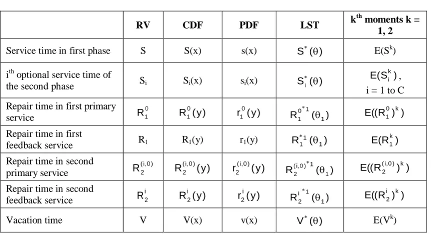
The notations of Random Variables (RV), Cumulative Distribution Function (CDF), Probability Density Function (PDF), Laplace-Stieltjes Transform (LST) and its kth moments of the RVs are listed below :

Table 1.1.1.

RV CDF PDF LST k

th

moments k = 1, 2

Service time in first phase S S(x) s(x) E(Sk)

ith optional service time of

the second phase Si Si(x) si(x)

, i = 1 to C

Repair time in first primary service

Repair time in first

feedback service R1 R1(y) r1(y)

Repair time in second primary service

Repair time in second feedback service

Vacation time V V(x) v(x) E(Vk)

Let NS(t) denote the system size at time t and

respectively denote the remaining times of the random variables ; service time in first stage,

second stage, repair time in first fresh service, first feedback service, second fresh service, second feedback service and vacation time at time t. Further the server states are denoted by the random variable Y(t) at time t.

Then the state space is {NS(t), (t)} where (t) = (0,

according as Y(t) = 0, 1, 2, 3, 4, 5, 6 and 7 respectively. The following joint probability

functions are defined, for further analysis of the model.

P(t) = Pr {NS(t) = 0, Y(t) = 0}, when the server is idle.

For n  1 and 1 i C

= Pr {NS(t) = n, x <  x + dt, Y(t) = 1}, a customer is being served in the

primary first phase service

P1,n(x, t) dt = Pr {NS(t) = n, x <  x + dt, Y(t) = 1}, a customer is being served in the first

phase – feedback service

) (

S 

) (

S_i  E(S )

k i

0 1

R R10(y) r (y)

0

1 R ( ₁)

1 0

1 



) ) R ((

E 01 k

) (

R 1

1

1 



) R (

E k1

) 0 , i ( 2

R R₂(i,0)(y) r₂(i,0)(y) _R ₍ ₎

1 1 ) 0 , i (

2 



) ) R (( E (₂i,0) k

i 2

R Ri₂(y) r₂i(y) _R ₍ ₎

1 1 i

2 



) ) R ((

E i₂ k

) (

V 

),

t

(

S



S

_i

(

t

),

(

R

₁0

)



(

t

),

(

R

₁

)



(

t

),

(

R

(₂i,0)

)



(

t

),

t

(

)

R

(

i₂ 

V



(

t

)

),

t

(

S



S

_i

(

t

),

(

R

₁0

)



(

t

),

(

R

₁

)



(

t

),

(

R

(₂i,0)

)



(

t

),

t

(

)

R

(

i₂ 

V



(

t

))

dt

t)

,

x

(

P

₁0_,_n

S



(

t

)

(4)

= Pr {NS(t) = n, x <  x + dt, Y(t) = 2}, a customer is being served in the ith

second phase primary service.

dt = Pr {NS(t) = n, x <  x + dt, Y(t) = 2}, a customer is being served in the ith

optional service of the second phase, during feedback.

= Pr {NS(t) = n, = x, y <  y + dt, Y(t) = 3}, a customer is waiting

for the first primary service due to breakdown.

BR1,n(x, y, t) dt = Pr {NS(t) = n, = x, y <  y + dt, Y(t) = 4}, a customer is waiting

for the first phase – feedback services due to breakdown.

For 1 iC ; n  1

for the second ith phase fresh service due to breakdown.

for the second ith phase service, during feedback due to breakdown.

Qn(x, t) dt = Pr {NS(t) = n, x <  x + dt, Y(t) = 7}, when the server is in vacation state.

(n 0)

1.1.1.2 System Size Distribution at Random Epoch

Observing the changes of states during the interval (t, t + t) for any time t, the steady state equations are given by :

System in Empty State

 P = Q0(0) + (1 – f) (1 – p)

Vacation State

 Qn(x) = Qn(x) +  (1 0,n) gk

+ (1 – f) p v(x) n  0

Busy with First Phase – Primary Service

 =  (+ ) + Pgn s(x) +

dt

t)

,

x

(

P

₂(i_,,_n0)

S

_i

(

t

)

t)

,

x

(

P

₂i_,_n

S

_i

(

t

)

dt

t)

y,

,

x

(

BR

₁0_,_n

S



(

t

)

(

R

0₁

)



(

t

)

t

(

S



(

R

₁

)



(

t

)

dt

t)

y,

,

x

(

BR

(₂i,_,_n0)

S

_i

(

t

)

(

R

(₂i,0)

)



(

t

)

dt

t)

y,

,

x

(

BR

i₂_,_n

S

_i

(

t

)

(

R

i₂

)



(

t

)

t

(

V



))

0 (

P

)

0 (

(P

_2,1i

C

1 i

(i,0)

2,1







x

d



 

n

1 k

k

n

(

x

)

Q

))

0 (

P

)

0 (

(P

2,in 1

C

1 i

) 0 , i (

1 n

2, 

 





x

d

)

x

(

P

₁0_,_n

a

10

P

(

x

)

0 n ,

1

BR

(

x

,

0)

(5)

+ (1 – f) (1 – p) s(x) + Qn(0) s(x)

+  (1 1,n) gk

Busy with First Phase Feedback Service

 P1,n(x) =  ( + a1) P1,n(x) + BR1,n(x, 0) + f1 s(x)

+ (1 1,n)  gk

Busy with Second Phase Primary Service

 =  (+ ) + (1 – 1,n)  gk

+ ri Si(x) + 1 i C, n  1

Busy with Second Phase Feedback Service (1 i C)

 =  (+ ) +  (1 – 1,n) gk +

+ f2ri Si(x) + P1,n(0) ri Si(x),

Breakdown in First Phase Fresh Service

 =  +  (1 1,n) gk

+ , (n  1)

Breakdown in First Phase Feedback Services

 BR1,n(x, y) =  BR1,n(x, y) +  (1 1,n) gk

+ a1 r1(y) P1,n(x), n  1 Breakdown in Second Phase Primary Service

 =  + (1 1,n) gk

))

0 (

P

)

0 (

(P

2,in 1

C

1 i

) 0 , i (

1 n

2, 

 







 

1 n

1 k

0 k n

1,

(

x

)

P

x

d

))

0 (

P

)

0 (

(P

2,in

C

1 i

(i,0) n

2,











 

1 n

1 k

k n

1,

(

x

)

P

x

d

)

x

(

P

₂(i_,,_n0)

a

(₂i,0)

P

₂(_.i,_n0)

(

x

)





 

1 n

1 k

) 0 , i (

k n

2,

(

x

)

P

)

0 (

P

₁_,_n

BR

(₂i_,,_n0)

(x,

0),

x

d

)

x

(

P

₂i_,_n

a

i₂

P

₂i_,_n

(

x

)





 

1 n

1 k

i k n

2,

(

x

)

P

BR

i₂_,_n

(x,

0)

))

0 (

P

)

0 (

(P

_2,(_n,0) C

1 n 2,



_





y



y)

,

x

(

BR

0₁_,_n

BR

0₁_,_n

(

x

,

y)





 

1 n

1 k

0 k n

1,

(

x

,

y)

BR

0 1

a

r

₁0

(

y

)

P

₁0_,_n

(

x

)

y







 

1 n

1 k

k n

1,

(

x

,

y)

BR

y



y)

,

x

(

BR

(₂i,_,_n0)

BR

(₂i_,,_n0)

(

x

,

y)





 

1 n

1 k

) 0 , i (

k n

2,

(

x

,

y)

(6)

+ , 1 i C

Breakdown in Second Phase Feedback Services

 =  + (1 1,n) gk

+ , 1 i C

The LST of the Steady-State equations are given by

 P = Q0(0) + (1 – f) (1 – p) (1.0)

 Qn(0) =   (1 0,n) gk

 (1 – f) p n  0 (1.1)

  = (+ )  Pgn 

 (1 – f) (1 – p)

Qn(0)  (1 1,n) gk (1.2)

  P1,n(0) = (+a1)   f1

 (1 1,n)  gk (1.3)

  = (+ )  (1 1,n)  gk

– ri – , 1 i C (1.4)

  = ( +  (1 1,n)  gk

– – f2ri )

0 , i ( 2

a

r

₂(i,0)

(

y

)

P

₂(i_,,_n0)

(

x

)

y



y)

,

x

(

BR

i₂_,_n

BR

i₂_,_n

(

x

,

y)





 

1 n

1 k

i k n

2,

(

x

,

y)

BR

i 2

a

r

₂i

(

y

)

P

₂i_,_n

(

x

)

))

0 (

P

)

0 (

(P

_2,1i

C

1 i

(i,0)

2,1







)

(

Q

_n



Q

_n

(



)



 





n

1 k

k

n

(

)

Q

))

0 (

P

)

0 (

(P

2,in 1

C

1 i

(i,0) 1 n

2, 

 





V



(



)

(

P

₁0_,_n



P

₁0_,_n

(

0 )

a

10

P

10,n

(



)



_S



₍

_

₎

0)

,

(

BR

₁0_,_n



))

0 (

P

)

0 (

(P

_2,i_n ₁

C

1 i

(i,0) 1 n

2, 

 





S



(



)

(

S









 





1

n

1 k

0 k n

1,

(

)

P

)

(

P

₁_,_n



P

₁_,_n

(



)

BR

₁_,_n

(



,

0)

(P

(

0 )

P

_2,i_n

(

0 ))

C

1 i

(i,0) n

2,







)

(

S







 

 



1

n

1 k

k n

1,

(

)

P

)

(

P

₂(i_,,_n0)



P

₂(_,i_n,0)

(

0 )

a

(2i,0)

P

(

)

) 0 , i (

n ,

2





)

(

P

1 n

1 k

) 0 , i (

k n ,

2





 

 

)

0 (

P

₁0_,_n

S

_i

(



)

BR

₂(i_,,_n0)

(



,

0)

)

(

P

2i,n





)

0 (

P

2i,n

a

)

i

2

P

(

)

i n ,

2



 n 1

_P

₍

₎

1 k

i k n ,

2





 

 

0)

,

(

BR

₂i_,_n



(P

(

0 )

P

_2,(_n,0)

(

0 ))

C

1 n 2,



_





(7)

 P1,n(0) ri 1 i C (1.5)

1  =  (1– 1,n) gk

 (1.6)

1  =  (1 – 1,n) gk  a1 (1.7)

1  = 

 (1 – 1,n) gk

 (1.8)

1  =  (1–1,n) gk

 (1.9)

1.1.3 Probability Generating Functions

The following partial PGFs are introduced to analyse the model :

= , Q(z, 0) =

= , =

= , P1(z, 0) =

= , =

= , = 1 i C

= , =

)

(

S

_i



)

,

(

BR

₁0_,_n1



₁

_BR

0

₍

_,

₀₎

n ,

1





_BR

₍

_,

₎

1 0

n ,

1 1





_





 





1

n

1 k

1 0

k n

1,

(

,

)

BR

1

0 1

a

R

0₁1

(



₁

)

_P

0

₍

₎

n ,

1





)

,

(

BR

1,n 1

1



 

0)

,

(

BR

1,n





)

,

(

BR

1,n 1

1





_



  





1

n

1 k

1 k n

1,

(

,

)

BR

1

)

(

R

₁1



₁

)

(

P

₁_,_n



)

,

(

BR

(₂i,_,_n0)1



₁

_BR

(i,0)

₍

_,

₀₎

n ,

2





)

,

(

BR

(₂i_,,_n0)1



₁



 

  



1

n

1 k

1 )

0 , i (

k n

2,

(

,

)

BR

1

) 0 , i ( 2

a

R

(₂i,0)1

(



₁

)

(

P

₂(i_,,_n0)



)

,

(

BR

i₂_,_n1



₁

_BR

i

₍

_,

₀₎

n ,

2





_BR

₍

_,

₎

1 i

n , 2

1





_



  





1

n

1 k

1 i

k n

2,

(

,

)

BR

1

i 2

a

R

i₂1

(



₁

)

(

P

2i,n





)

,

z

(

Q





n

0 n

n

(

)

z

Q



 



_

n

0 n

n

(

0 )

z

Q



 

)

,

z

(

P

₁0



n

1 n

0 n

1,

(

)

z

P



 



_

_P

0

₍

_z

_,

₀

₎

1

n

1 n

0 n

1,

(

0 )

z

P



 

)

,

z

(

P

₁



n

1 n

n

1,

(

)

z

P



 



_

n

1 n

n

1,

(

0 )

z

P



 

)

,

z

(

P

₂(i,0)



n

1 n

(i,0) n

2,

(

)

z

P



 





P

₂(i,0)

(z,

0)

n

1 n

(i,0) n

2,

(

0 )

z

P



 

)

,

z

(

P

₂i



n

1 n

i n

2,

(

)

z

P



 



_

_P

i

_(z,

₀₎

2

n

1 n

i n

2,

(

0 )

z

P



 

)

,

z

(

BR

₁01



₁ n

1 1

n

0 n

1,

(

,

)

z

BR

1





 

 

0)

,

z

(

BR

₁0



n

1 n

0 n

1,

(

,

0)

z

BR



 

(8)

= , =

Multiplying the corresponding equations by suitable powers of z and adding the equations, partial generating functions are derived, through some algebraic manipulations. Equation (1.1) implies

(wX(z)) = Q(z, 0) 

At  = wX(z),

Q(z, 0) = , hence (1.10)

= (1.11)

The partial probability generating functions of the system size, when the server is in breakdown state during first stage (primary service and feedback services) services are obtained using the equations (1.6) and (1.7) given by,

= (1.12)

= (1.12.1)

= a1 (1.13)

= (1.13.1)

The partial probability generating functions of the system size, when the server is in breakdown state during second stage (primary and feedback) services are obtained using the equations (1.8) and (1.9) and given by,

= (1.14)

= (1.15)

= (1.16)

)

,

z

(

BR

₁1



₁ n

1 1

n

1,

(

,

)

z

BR

1





   

0)

,

z

(

BR

₁



n

1 n

n

1,

(

,

0)

z

BR



 



)

,

z

(

BR

(₂i,0)1



₁ ₁ n

1 n ) 0 , i ( n

2,

(

,

)

z

BR

1





   

0)

,

z

(

BR

(₂i,0)



n

1 n ) 0 , i ( n

2,

(

,

0)

z

BR



 



)

,

z

(

BR

i₂1



₁ n

1 1

n i

n

2,

(

,

)

z

BR

1





   

0)

,

z

(

BR

i₂



n

1 n

i n

2,

(

,

0)

z

BR



 



)

,

z

(

Q





z

)

(

V

p

f)

1 (







))

0 ,

z

(

P

)

0 ,

z

(

(P

₂(i,0)

C 1 i i 2







z

))

z

(

w

(

V

p

f)

1 (



 _X

))

0 ,

z

(

P

)

0 ,

z

(

(P

₂(i,0)

C 1 i i 2







)

,

z

(

Q





z

p

f)

1 (



))

z

(

w

(

))

(

V

))

z

(

w

(

(V

X X







 

))

0 ,

z

(

P

)

0 ,

z

(

(P

₂(i,0)

C 1 i i 2







0)

,

z

(

BR

₁0



a

₁0

P

₁0

(

z

,



)

R

0₁1

(

w

_X

(z))

)

,

z

(

BR

₁1



₁

_a

_P

0

₍

_z

_,

₎

1 0 1





))

z

(

w

(

)]

(

R

))

z

(

w

(

[R

X 1 1 0 1 X 0

1 1 1







 

0)

,

z

(

BR

₁



P

₁

(

z

,



)

R

₁1

(

w

_X

(z))

)

,

z

(

BR

₁1



₁

_a

_P

₍

_z

_,

₎

1 1





))

z

(

w

(

)]

(

R

))

z

(

w

(

[R

X 1 1 1 X

11 1







 

0)

,

z

(

BR

(₂i,0)



a

(₂i,0)

P

₂(i,0)

(

z

,



)

R

₂(i,0)1

(

w

_X

(

z

))

)

,

z

(

BR

1 ) 0 , i ( 2 1



 

))

z

(

w

(

)]

(

R

))

z

(

w

(

R

[

)

,

z

(

P

a

X 1 1 ) 0 , i ( 2 X ) 0 , i ( 2 ) 0 , i ( 2 ) 0 , i ( 2 1 1









  

0)

,

z

(

BR

i₂



a

i₂

P

₂i

(

z

,



)

R

(

w

X

(

z

))

i

2

(9)

= (1.17)

Equation (1.4) gives the generating functions of the system size when the server is busy with second stage fresh service, at the service completion epoch and at arbitrary epoch :

= ri (1.18)

where = wX(z) + (1 – (wX(z))) (1.18.1)

= ri (1.19)

Similarly Equation (1.5) gives the generating functions of the system size when the server is busy with second stage ith feedback service, at the service completion epoch and at arbitrary epoch :

= ri [f2 + P1(z, 0)] (1.20)

= [f2 +P1(z, 0)]

(1.21)

where = wX(z) + (1 – (wX(z))) (1.21.1)

The equations (1.14) to (1.21) are obtained for 1 i C.

Adding the equations (1.18) and (1.20) over i = 1 to C,

= (1.22)

where k0(z) = (1.23)

and k(z) = (1.23.1)

The PGF corresponding to the state, when the server is busy in first stage feedback service, is obtained by using the equation (1.3) as,

( = P1(z, 0) – f1 (1.24)

)

,

z

(

BR

i₂1



₁

))

z

(

w

(

)]

(

R

))

z

(

w

(

R

[

)

,

z

(

P

a

X 1

1 i 2 X

i 2 i

2 i 2

1 1









 



0)

,

z

(

P

₂(i,0)

P

₁0

(

z

,

0)

S

_i

(

h

_a ₍_i_,₀₎

(

w

_X

(

z

)))

2



))

z

(

w

(

h

_a ₍_i_,₀₎ _X

2

) 0 , i ( 2

a

(i,0) 1

2

R



)

,

z

(

P

₂(i,0)



P

₁0

(

z

,

0)

)))

z

(

w

(

h

(

))

(

S

)))

z

(

w

(

h

(

S

(

X ) 0 , i ( a

i X

) 0 , i ( a i

2 2







 

0)

,

z

(

P

₂i

S

_i

(

h

_ai

(

w

_X

(

z

)))

2



))

0 ,

z

(

P

)

0 ,

z

(

(P

(

₂( ,0)

C

1 2



_





)

,

z

(

P

₂i



)))

z

(

w

(

h

(

))

(

S

)))

z

(

w

(

h

(

S

(

r

X a

i X

a i i

i 2 i 2







 

))

0 ,

z

(

P

)

0 ,

z

(

(P

(

₂( ,0)

C

1 2



_





))

z

(

w

(

h

_ai _X

2

i 2

a

i 1

2

R



))

0 ,

z

(

P

)

0 ,

z

(

(P

(

₂

C

1 ) 0 , ( 2



_





1 f

k(z)

0)

,

z

(

P

k(z)

0)

,

z

(

P

(z)

k

2

1 0





)))

z

(

w

(

h

(

S

r

_X

a i C

1 i

i (i,0)

2







)))

z

(

w

(

h

(

S

r

_i _a _X

C

1 i

i i

2







)))

z

(

w

(

h

_a _X

1

P

1

(

z

,



)



)

(

S





(

(P

(

z

,

0 )

P

₂(i,0)

(

z

,

0 ))

C

1 i

i

2



(10)

Using the equation (1.22) in (1.24) and simplifying, we have at  =

P1(z, 0) = (1.25)

Substituting the value of P1(z, 0) in (1.24) and simplifying we get

= (1.26)

Using the equations (1.22) and (1.25) in (1.11),

=

(1.26.1)

Next to calculate the PGF corresponding to the state when the server is busy in first stage fresh service, the equation (1.2) is used and it is found that,

 

= (+ )  P X(z) 

 (1 – f) (1 – p)

X(z)  [Q(z, 0) – Q0(0)] (1.27)

The equations (1.12), (1.22), (1.0), (1.10) together with (1.27) give

(

= + PwX(z) (1.28)

At =

= (1.29)

)),

z

(

w

(

h

_a _X

1

))))

z

(

w

(

h

(

S

f

(f

k(z)

1 0)

,

z

(

P

)

z

(

k

)))

z

(

w

(

h

(

S

f

X a 1 2 0 1 0 X a 1 1 1  





)

,

z

(

P

₁



))))

z

(

w

(

h

(

S

f

(f

k(z)

1 0)

,

z

(

P

)

z

(

k

f

X a 1 2 0 1 0 1 1 





(

h

(

w

(

z

)))

))

(

S

)))

z

(

w

(

h

(

S

(

X a X a 1 1







 

)

,

z

(

Q





z

p

f)

1 (



))))]

z

(

w

(

h

(

S

f

(f

k(z)

[1

0)

,

z

(

P

)

z

(

k

X a 1 2 0 1 0 1 





(

w

(

z

))

(

V

)))

z

(

w

(

V

(

X X







 

)

,

z

(

P

₁0



P

₁0

(

z

,

0)

0 1

a

P

₁0

(

z

,



)

S



(



)

BR

₁0

(

z

,



,

0)

z

)

(

S











C 1 i (i,0) 2,1 (i,0)

2

(

z

,

0 )

P

(

0 )

z

[P



P

₂i

(

z

,

0 )



P

_2,1i

(

z

,

0 )

z

]

)

,

z

(

P

₁0



S



(



)

)))

z

(

w

(

h

_a0 _X

1

)

,

z

(

P

₁0



0)

,

z

(

P

₁0





























   

)))])

z

(

w

(

h

(

S

f

[f

k(z)

(1

z

)]

z

(

k

)))

z

(

w

(

V

p

(1

f)

(1

)

(

S

))))]

z

(

w

(

h

(

S

f

(f

k(z)

1 [

z

[

X a 1 2 0 X X a 1 2 1 1

)

(

S





))

z

(

w

(

h

0_a _X

1

0)

,

z

(

P

₁0

(11)

where = [1 – k(z) (f2 + f1 ]

and = z  (1–f) (1–p + p k0(z) (1.30)

Substituting (1.29) in (1.28) and simplifying we get

= (1.31)

Thus the partial generating functions corresponding to different states at arbitrary epochs are calculated using the respective equations and are given by :

= (1.32.1)

= (1.32.2)

For 1i C,

= (1.32.3)

= (1.32.4)

= (1.32.5)

= (1.32.6)

= (1.32.7)

= (1.32.8)

))

z

(

w

(

S

_F _X

S

(

h

a1

(

w

X

(

z

))))



)

z

(

D

₁BV_,_IF

S

_F

(

w

_X

(

z

))

S

(

h

_a0

(

w

_X

(

z

)))

1 

)))

z

(

w

(

V

 _X

)

,

z

(

P

₁0



)))

z

(

w

(

h

(

)

z

(

D

)))]

z

(

w

(

h

(

S

)

(

[S

(z))

(w

S

z

P

)

z

(

w

X a BV F , 1 X a X F X 0 1 0 1











   

0)

,

z

(

P

₁0

))

z

(

w

(

h

)

z

(

D

]

1 )))

z

(

w

(

h

(

S

[

(z))

(w

S

)

z

(

w

P

z

X a BV F , 1 X a X F X 0 1 0 1   

_



0)

,

z

(

P

₁

))

z

(

w

(

h

)

z

(

D

1)

)))

z

(

w

(

h

(

S

(

)))

z

(

w

(

h

(

S

(z)

k

f

)

z

(

w

P

z

X a BV F , 1 X a X a 0 1 X 1 1 0 1   

_



0)

,

z

(

P

₂(i,0)

))

z

(

w

(

h

)

z

(

D

]

1 )))

z

(

w

(

h

(

S

[

(z))

(w

S

)))

z

(

w

(

h

(

S

r

))

z

(

w

(

P

z

X a BV F , 1 X a i X F X a i X ) 0 , i ( 2 ) 0 , i ( 2 0 1    

_



0)

,

z

(

P

₂i

))

z

(

w

(

h

)

z

(

D

]

1 )))

z

(

w

(

h

(

S

[

)))]

z

(

w

(

h

(

S

f

[f

)))

z

(

w

(

h

(

S

(z)

k

r

)

z

(

w

P

z

X a BV F , 1 X a i X a 1 2 X a 0 i X i 2 i 2 1 0 1    

_

_



0)

,

z

(

Q



)

z

(

D

)

1 ))

z

(

w

(

V

(

)))

z

(

w

(

h

(

S

(z)

k

p

f)

(1

P

BV F , 1 X X a 0 0 1   

_





0)

0,

,

z

(

BR

₁01

)

z

(

w

)))

z

(

w

(

R

(1

0)

,

z

(

P

a

X X 0 1 0 1 0 1 1  



0)

0,

,

z

(

BR

1 1  

)

z

(

w

)))

z

(

w

(

R

(1

0)

,

z

(

P

a

X X 1 1 1 1  

_

0)

0,

,

z

(

BR

(₂i,0)1

(12)

= (1.32.9)

where , k(z), k0(z) are given by the equations (1.30), (1.23.1) and (1.23) respectively.

To derive the total PGF of the system size distribution, the following generating functions are considered.

PIdle(z) = Probability generating function of the system size when the server is idle in idle state

= P +

= [z  (1 – f) k0(z)] (1.33)

PComp(z) = The PGF of the system size when server is busy or in breakdown state

= + + +

+ + + + =

[ k0(z) (1 – f) – (1.34)

Thus the total PGF of the system size distribution is given by = PIdle(z) + PComp(z)

= (1.35)

where is given by the equation (1.30). P can be calculated by using the normalizing condition

= 1 and found to be P = 1 – where

(1.36)

= E(X)[pE(V)+ + + + E(H1)] (1.37)

The measures E(H) s’ are obtained from the LST of random variables,

= =

= = for 1 i C,

0)

0,

,

z

(

BR

i₂1

)

z

(

w

)))

z

(

w

(

R

(1

0)

,

z

(

P

a

X

X i

2 i

2 i 2

1

 



)

z

(

D

BV1,F

0)

,

z

(

Q



)

z

(

D

P

BV

F ,

1



(z))

(w

S

_F _X

S

(

h

_a0

(

w

_X

(

z

)))

1



0)

,

z

(

P

₁0

BR

₁01

(

z

,

0,

0)

P

₁

(

z

,

0)

BR

1

(

z

,

0,

0)

1

 





 C

1 i

(i,0)

2

(

z

,

0)

[P

BR

₂(i,0)1

(

z

,

0,

0)

P

₂i

(

z

,

0)

BR

i₂1

(

z

,

0,

0)]

)

z

(

D

z

P

BV

F ,

1



)))

z

(

w

(

h

(

S

_X

a0₁



_S

₍

_w

₍

_z

_)]

X F 

)

z

(

P

_BV_F

)

z

(

D

)))

z

(

w

(

h

(

S

)

z

(

k

f)

(1

1)

(z

P

BV F , 1

X a

0 0

1

 





)

z

(

D

₁BV_,__F

)

1 (

P

_BV_F



BV₁_,__F

BV F , 1



E

(

H

₁0

)

f

1 f





_ C

1 i

i

r

E

(

H

i₂

)



 C

1 i

i

r

E

(

H

(₂i,0)

)

f

1 f

₁



)

z

(

H

₁

S

(

h

_a

(

w

_X

(

z

))),

1



_H

0

₍

_z

₎

1 

))),

z

(

w

(

h

(

S

_a0 _X

1



)

z

(

H

i₂

S

(

h

(

w

_X

(

z

))),

a

i i

2



_H

i,0

₍

_z

₎

2



)))

z

(

w

(

h

(

S

_X

a

i (i,0)

2

(13)

and are given by :

E(H1) = E(S) (1 + a1 E(R1)) (1.37.1)

= E(S) (1 + (1.37.2)

= E(Si) (1 + (1.37.3)

= E(Si) (1 + (1.37.4)

= E(S) a1 + E(S2) (1 + a1 E(R1))2 (1.37.5)

= E(S) + E(S2) (1 + (1.37.6) = E(Si) + (1+ (1.37.7)

= E(Si) + (1 + (1.37.8)

Hence

= (1.38)

8.1.1.4 Decomposition Property

Using equation (1.33), equation (1.38) can be re-written as

= (1.39) where

1,F =  E(X) [ + + + E(H1)] (1.40)

=  p  E(X) E(V)

and ,E(H1), , are given by the equations (1.38.1) to (1.38.4).

Under the steady state condition < 1, the PGF of the stationary system size of the queueing model under

consideration is the product of the PGF of the system size of MX/G,Gi(1 i C) /1 queueing system with infinite feedback and service interruption (without vacation) and the distribution of the conditional system size during the idle period given that the server is idle.

)

H

(

E

₁0

a

₁0

E

(

R

₁0

))

)

H

(

E

(₂i,0)

a

(₂i,0)

E

(

R

(₂i,0)

))

)

H

(

E

i₂

a

i₂

E

(

R

i₂

))

)

H

(

E

₁2

E

(

R

₁2

)

H

((

E

0₁ 2

a

₁0

E

((

R

0₁

)

2

)

a

₁0

E

(

R

₁0

))

2

)

H

((

E

(₂i,0) 2

a

₂(i,0)

E

((

R

₂(i,0)

)

2

)

E

(

S

2_i

)

a

(₂i,0)

E

(

R

(₂i,0)

))

2

)

H

((

E

i₂ 2

a

i₂

E

((

R

i₂

)

2

)

E

(

S

_i2

)

a

i₂

E

(

R

i₂

))

2

)

z

(

P

_BV_F

)

z

(

D

)))

z

(

w

(

h

(

S

)

z

(

k

f)

(1

1)

(z

)

1 (

BV F , 1

X a 0

BV F ,

1 0

1













)

z

(

P

_BV_F

]

k

f)

(1

)))

z

(

w

(

h

(

S

))

z

(

w

(

S

z

[

)))

z

(

w

(

h

(

S

)

z

(

k

f)

(1

)

1 (

1)

(z

0 X

a X

F

X a 0

F , 1

0 1







 

 













)

1 (

P

)

z

(

P

Idle Idle

)

H

(

E

₁0

r

E(H

(i,0)₂

)

C

1 i

i





1 f

f





 C

1 i

i

r

E

(

H

i₂

)

f

1 f

₁



BV IF , 1



)

H

(

E

₁0

E

(

H

i₂

)

E

(

H

(₂i,0)

)

(14)

1.1.5 Queue Size Distribution at Departure Epoch

If denotes the probability that there are n customers in the system at departure epoch, then =

D1 [(1 – f) , with the normalizing constant D1.

The PGF +(z) of the queue size distribution { ; n  0} at departure epoch is given by

+

(z) = zn = (1 – f) = (X(z) – 1)

(from (1.20) and (1.18) Evaluating D1 using normalizing condition, +(z) =

1.1.6 Performance Measures

(i) The probability that the server is on vacation state (PV) is

PV = = p E(X) E(V)

(ii) The probability that the server is busy is Pbusy = + P1 +

=

(iii) The probability that the server is in breakdown state (Pbr) is obtained by,

Pbr =

=  E(X)





_n

_



n

)]

0 (

P

)

0 (

P

2,in 1

C

1 i

(i,0) 1 n

2, 

 









_n



 





0 n

n

z

D

₁

))

0 ,

z

(

P

)

0 ,

z

(

(P

2i

C

1 i

(i,0)

2







z

1 D

₁



P

(

z

)

BV F 

1)

(z

)

X

(

E

1)

)

z

(

X

(



)

z

(

P

_BV_F

1

z

lim



Q

(

z

,

0)



0 1

P







C

1 i

i 2 (i,0)

2

P

)

(P

1

z

lim





_













 



 

 C

1 i

i 2 C

1 i

(i,0) 2 1

0

1

(

z

,

0)

P

(

z

,

0)

P

(

z

,

0)

P

(

z

,

0)

P

f

1 E(X)























 C

1 i

i i

2

)

r

E(S

)

f

(1

)

S

(

E

1

z

lim





_













 C

1

i br br

br

P

(P

P

)

P

i

2 (i,0) 2 1

0 1

)]

E(R

a

f

1 f

)

E(R

[a

)

S

(

E

₁0 0₁ 1 ₁ ₁





























_



)

E(R

a

f

1 f

)

E(R

a

)

E(S

r

(i,0)₂ (i,0)₂ i₂ i₂

C

1 i

(15)

(iv) The expected system size for the model is given by

= =E(X) [ + + (1.41) where is given by the equation (1.37) and

=  E(X(X–1) [f + f1 E(H1) + (1–f) [ + pE(V) + +(E(X))2{f

+f1 +(1–f)[ +pE(V2)+ + 2[ f1E(H1)

+(1–f)[pE(V) +(pE(V)+ ) + 2  E(X) [f + f1 E(H1)]

where E(H1), , , , , , , are given by

the equations (1.37.1) to (1.37.8).

1.2 PARTICULAR CASES

The model of the present section considers the case in which, the customers when discontented with their services may either demand re-service from phase 1 followed by phase 2 with probability (f1) (or) demand re-service of phase 2 type alone with probability f2 (or) leave the system with probability 1 – (f1 + f2) = 1 – f, without demanding re-services.

Case 1:

If f1 = 0 (i.e., f2 = f), then the PGF of the system size of the model, in which the feedback

customers demand re-services only of phase 2 type is obtained from equation (1.38) and given by

= (1.42.1)

where,

=  E(X) (1.42.2)

Case 2 :

If f2 = 0 then the PGF of the system size of the model in which all the feedback customers repeat services from phase 1 followed by phase 2 is obtained from equation (1.38) and given by

BV F

L

_

1 z BV

F

(

z

)

(P

z

d

 









)

H

(

E

₁0



 C

1 i

(i,0) 2

i

E(H

)]

r

)

(1

f)

(1

2 ))

1 (

D

(

BV F 1, BV

F 1,

 









BV F , 1



))

1 (

D

(



BV_1,__F



)

E(H

r

i₂ C

1 i

i





)

H

(

E

₁0

r

E(H

(i,0)₂

)]]

C

1 i

i





)

E((H

r

i₂ 2 C

1 i

i





)

H

(

E

₁2

E

((

H

₁0

)

2

)

r

E((H

(i,0)₂

)

2

)]

C

1 i

i





)

E(H

r

i₂ C

1 i

i





)

H

(

E

₁0

E

(

H

₁0

)

r

E((H

(i,0)₂

))]]}

C

1 i

i





)

E(H

r

i₂ C

1 i

i





)

H

(

E

₁0

E(H

i₂

)

E(H

(i,0)₂

)

E

(

H

₁2

)

E

((

H

₁0

)

2

)

E((H

i₂

)

2

)

E((H

(i,0)₂

)

2

)

z

(

P

₁BV_,_IF

k(z)

f

1 )

z

(

k

)))

z

(

w

(

V

p

(1

f)

(1

)))

z

(

w

(

h

(

S

z

k(z)

f

1 )

z

(

k

)))

z

(

w

(

h

(

S

f)

(1

1(

(z

)

1 (

0 X

X a

0 X

a BV

IF 1,

0 1











 



BV IF , 1



_











_











E(V)

p

)

E(H

)

E(H

r

)

E(H

r

f

1 f

0

1 C

1 i

i,0 2 i C

1 i

(16)

=

(1.43.1) =  E(X)

If we assume that, the probability with which the server takes vacation after the completion of each service (p) is zero, the arrivals follow simple Poisson process (E(X) = 0) and the server never breaks down (ai = 0), then equations (1.23) and (1.23.1) give :

k0(z) = k(z) ; = =

and P(z) = (1.44)

where = (E(S) + and A(z) = k(z)

it is verified that under the condition m , (1.44) coincides with the PGF of the system size of the two phase service reliable M/G/1 queueing model (with finite number of immediate feedback) analysed by Kalidass and Kasturi (2013).

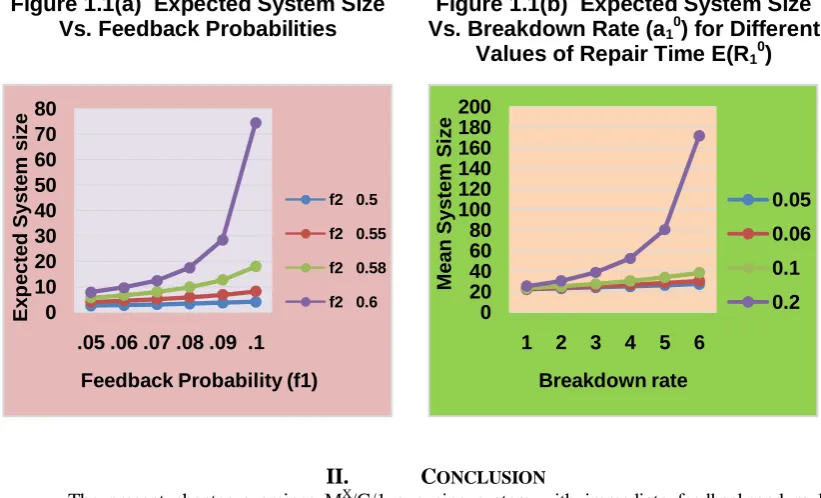
NUMERICAL ANALYSIS

In this section numerical results are obtained to study the effects of (i) the probability that the server chooses feedback service from first phase (f1) or from second phase (f2), (ii) the

breakdown rates, (iii) mean repair time on the expected system size for the present model. The different distributions assumed are presented in the following table.