Biotools: an R function to predict spatial gene diversity via an individual-based approach.

(1)

Biotools: an R function to predict spatial gene

diversity via an individual-based approach

A.R. da Silva1_{, G. Malafaia}2_{and I.P.P. Menezes}3

1_{Laboratório de Estatística Aplicada, Instituto Federal Goiano, Urutaí, GO, Brasil} 2_{Laboratório de Pesquisas Biológicas, Instituto Federal Goiano, Urutaí, GO, Brasil} 3_{Laboratório de Genética Molecular, Instituto Federal Goiano, Urutaí, GO, Brasil}

Corresponding author: A.R. da Silva E-mail: [email protected]

Genet. Mol. Res. 16 (2): gmr16029655 Received February 23, 2017

Accepted March 14, 2017 Published April 13, 2017

DOI http://dx.doi.org/10.4238/gmr16029655

ABSTRACT. The gene diversity or expected heterozygosity (H_E) is based on the allele frequency and is often used as a measure of genetic variability of populations. Knowing the pattern of spatial distribution of H_E can be useful for determining strategies of conservation and sampling of collections of individuals. In addition, it can allow one to detect genetic boundaries in a landscape. We adapted a Wombling method based on assignment tests in a circular moving window extensively sampled over the study area in order to estimate H_E at points of a prediction grid. The function sHe(), package biotools, is

an easy-to-use and flexible implementation in R language that accepts

as input geographical and genotyping data. The package biotools is distribution-free under the GPL-2/3 license and currently available from the Comprehensive R Archive Network (CRAN) at http://CRAN.R-project.org/package=biotools. The R platform and all R dependencies are similarly available from CRAN.

(2)

INTRODUCTION

The gene diversity or expected heterozygosity (H_E) is a parameter often employed to quantify the genetic variability within a population or species. This parameter has been the base for evaluating the relationship between population genetic diversity and the effective number of alleles, in order to detect intra- and inter-populational endogamy, for measuring the linkage disequilibrium and to test for natural selection occurrence (Frankham et al., 2004; Hartl and Clark, 2010). H_E is based on the polymorphic allele pool of a population; its unbiased estimator, as presented by Nei (1978), is given by:













₋

−

=

∑

i

p

i

n

e

H

₁

2

1

2

2 ˆ

_{(Equation 1)}

where n is the number of individuals in a population and p_i is the relative frequency of the i-th allele in a certain locus in this population. The classical and most frequent use of H_E is with

populations or predefined groups of individuals. It can be calculated for a certain DNA marker

or more generally as the mean value of Equation 1 across all markers used to characterize a population.

Studying the spatial distribution of H_E allows one to analyze the occurrence of hot-spots of genetic diversity over a landscape. The data analysis of DNA markers, combined with phenotypic and spatial data, can be particularly useful to promote fundamental insights on the evolutionary history, natural selection, adaptation and domestication of species (Rodriguez et al., 2016). Moreover, the spatial genetic variation is useful for conservation management of accessions in breeding programs. For this purpose, spatial interpolation techniques such as kriging appear as tools for obtaining associating interpretations between the phytophysiognomy and the evolutionary dynamics of populations. In this context, genetic diversity heat maps can be very elucidative (Corre et al., 1998).

Manel et al. (2007) presented a Wombling method to identify genetic boundaries via a spatial approach that consists of assignment tests in a circular moving window over an extensively sampled study area, making it possible to identify locations where abrupt changes on allele frequency occur. This technique avoids assumptions of discrete genetic groups and may be particularly useful for animals or plants that have non-clumped or uniform distributions (Storfer et al., 2010). Nevertheless, the availability of this method in software packages is still restricted. We have adapted and implemented this procedure in R language (http://www.R-project.org/) in an efficient and flexible way with the intention of predicting H_E at points of a predetermined spatial grid. The function sHe() of the package biotools (version 3.0) allows one to obtain spatial unbiased estimates of gene diversity from molecular datasets. In this paper, we detail the algorithm and the usage of sHe(). A video, distributed as Supplementary information (Appendix S1), illustrates the procedure.

MATERIAL AND METHODS

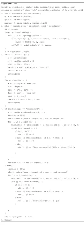
Algorithm

(3)

Thus, Step 1 of its algorithm (Figure 1) is to define the input: i) locations of sampling points,

ii) the matrix of geographical distances among sampling points, iii) the prediction grid, and iv) the marker data.

In Step 2, Euclidian distances between every sampling point and every point of the prediction grid are calculated and stored in the object ‘mdis’, a matrix with dimension n ×

m, where m is the number of predicting points. Afterwards, for each predicting point, those sampling points distant by the input ‘radius’ or less are computed and stored in the object ‘id’, a list of size m.

Auxiliary functions are written in Step 3 in order to estimate H_E for both codominant or dominant markers - ‘fHeco’ and ‘fHe’, respectively. This way of programming makes sHe() faster and easier to debug.

In Step 4, the type of marker defines how H_E is calculated through the auxiliary functions in Step 3. In both cases, a matrix containing the estimates of H_E per locus at each predicting point is computed. Afterwards, the mean value of H_E is calculated for each predicting point.

(4)

Features

As input, sHe() accepts for the argument “x” a numeric matrix or data frame organized in columns containing geographical coordinates and genotyping data. The latter can be obtained via codominant (default) or dominant molecular markers. The arguments “coord. cols” and “marker.cols” must be used to inform the columns in “x” corresponding to those

data. It is advised that the first column of coordinates is referring to the x-axis. An optional argument, “grid”, can be used to define a prediction grid, otherwise sHe() will automatically define a rectangular grid of dimension 50 × 50, considering the limits of the coordinates in “x”.

The user has the opportunity of dealing with coordinates in the Latitude-Longitude (degrees) system and even though to pass a radius for the search moving window in kilometres, i.e., without having to convert the coordinates before using the function. To do so, one just has to keep the argument latlong2km = TRUE; if FALSE, then the argument “radius” must receive a numeric value in the same unit as the input coordinates. Finally, the optional argument “nmin” restricts the calculation of H_E to locations where the search window of predetermined radius

finds out a fixed number of individuals.

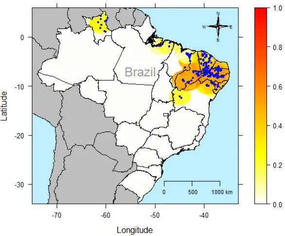
sHe() outputs an object of homonymous class that consists basically of a list containing: (i) a data frame with the coordinates of the prediction grid, the number of individuals found at each point of that grid, the unbiased estimate and the standard error of H_E; (ii) a numeric matrix containing values of H_E per locus for each point of the prediction grid. A print method summarizes the output. There is also a plot method for objects of class sHe, whose solution is a gene diversity heat map (Figure 2). For this, the package lattice (Sarkar, 2008) is used.

(5)

The function allows one to deal with missing values, i.e., “NA” values, which are disregarded on the calculation of allele frequency.

The program, user manual and examples are available on CRAN (http://CRAN.R-project.org/package=biotools).

RESULTS AND DISCUSSION

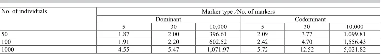
Prediction sites are analyzed by a loop. Thus, large datasets may increase the processing time. Timings for several analyses can be seen in Table 1. The number of markers is more time demanding than the number of individuals. Codominant markers take more time to compute

H_E than dominant, for the calculations involve twice the number of columns in the genotyping data set. And of course, the larger the grid size the more time demanding is the process.

Table 1. Timing for analyses performed with various data sizes.

No. of individuals Marker type  No. of markers

Dominant Codominant

5 30 10,000 5 30 10,000 50 1.87 2.00 396.61 2.09 3.77 1,099.81 100 1.91 2.20 602.52 2.42 4.70 1,556.43 1000 4.55 5.47 1,071.97 5.72 12.52 5,021.82 Time in seconds, based on Intel®_CoreTM_{i5 1.40 GHz, with 3.71 GB RAM. Analyses based on a prediction grid of}

dimension 50 x 50.

CONCLUSION

An effective and flexible tool for predicting gene diversity over a sampling area has

been created. The package biotools has been regularly updated and on permanent improvement.

ACKNOWLEDGMENTS

We thank Instituto Federal Goiano (Brazil) for the financial support.

REFERENCES

Corre VL, Rousse G, Zanetto A and Kremer A (1998). Geographical structure of gene diversity in Quercus petraea (Matt.)

Liebl. III. Patterns of variation identified by geostatistical analyses. Heredity 80: 464-473. http://dx.doi.org/10.1046/ j.1365-2540.1998.00313.x

Frankham R, Ballou JD and Briscoe DA (2004). A primer of conservation genetics. Cambridge University Press, New York.

Hartl DL and Clark AG (2010). Principles of population genetics. 4th edn. Artmed, Porto Alegre.

Manel S, Berthoud F, Bellemain E, Gaudeul M, et al.; Intrabiodiv Consortium (2007). A new individual-based spatial approach for identifying genetic discontinuities in natural populations. Mol. Ecol. 16: 2031-2043. http://dx.doi. org/10.1111/j.1365-294X.2007.03293.x

Nei M (1978). Estimation of average heterozygosity and genetic distance from a small number of individuals. Genetics

89: 583-590.

Rodriguez M, Rau D, Bitocchi E, Bellucci E, et al. (2016). Landscape genetics, adaptive diversity and population structure

in Phaseolus vulgaris.New Phytol. 209: 1781-1794. http://dx.doi.org/10.1111/nph.13713

Sarkar D (2008). Lattice: Multivariate Data Visualization with R. Springer, New York.

(6)

Supplementary material

Appendix S1. A video (video_she_SuppInfo.mpg) illustrating the algorithm of the spatial individual-based