Optimization of Remote Meteorological Parameters in Predicting the Air Pollutant (NO 2

115604-8282 IJET-IJENS @ August 2011 IJENS _{I J E N S}

Optimization of Remote Meteorological

Parameters in Predicting the Air Pollutant

(NO

₂

) Distribution by Petrochemical Industry

along Coastal Zone at East Coast of

Peninsular Malaysia

Mohd H. Ibrahim

, Ahmad M. Abdullah

, Nor M. Adam

, Juliana Jalaludin

,

W.M. Norhisyam W. Mamat

, Mohd N.Ibrahim

, Noraniah Abdul Aziz

1_{Faculty of Environmental Studies,} 2

Faculty of Mechanical and Manufacturing Engineering,

3_{Faculty of Medicine and Health Science,}

Universiti Putra Malaysia, 43000 UPM Serdang, Selangor. MALAYSIA

4_{Kolej Universiti TATI, Jalan Panchor, Teluk Kalong,}

24000 Kemaman, Terengganu, MALAYSIA Email: [email protected]

Abstract-- As commonly observed throughout the world, the meteorological parameters at coastal area are influenced by both rotation of wind direction and sea breezes wind vectors features. Theoretically, this atmospheric condition describes difficulties in predicting on ground concentration of pollutant using the acceptable method of dispersion under the turbulence properties. This research applies the air dispersion modeling using ISCT3 software in order to predict on ground concentration of NO2 from selected petrochemical plants in

Kertih, Terengganu, located at North East of Peninsular Malaysia Meteorological data of year 2008 obtained from the Kuala Terengganu Meteorology Station was used as input to the ISCT3 software. This meteorology station is located approximately 95 km north-west off the study site which contains the pollutant sources and verification point. The modeling domains covered a 20 x 20 km2 area centre of the petrochemical industry with grid spacing of 500 meter each as dummy receptors. During verification process, the significance improvement through the optimization analysis of wind direction proven that the correlation coefficient of predicted over the actual NO2 concentration improve from 0.68 to 0.91.

The average maximum monthly and yearly on ground concentration NO2 obtained is at 13.97 ug/m3 and 6.91 ug/m3

respectively. The annual value is much below the Malaysian and WHO guidelines which is at 90 ug/m3 and 40 ug/m3 respectively. No benchmarking could be gauged on the monthly value since no guideline is available.

Index Term - Air dispersion modeling, optimization analysis, correlation coefficient, NO2, ISCT3.

I. INTRODUCTION

AS COMMONLY observed throughout the world that the meteorological parameters at coastal area are influenced by

sea breezes [1] and both by rotation of wind direction and sea breezes wind vectors features [2]. It has been highlighted that it is hard to describe theoretically the acceptable method to predict pollutant dispersion under the turbulence properties [3] which this atmospheric condition could influence the concentration of air pollutant [4].

There are two types of sources of pollutants emissions; mobile sources and stationary sources [5]. Mobile sources are including highway vehicles and other mode of transportation while stationary sources are categorized as stationary fuel combustion and industrial processes. Generally, pollutants emitted controlled under the international standard are the NOx, O3, PM, SOx, and CO [6].

In Malaysia these pollutants are controlled by the Malaysian standard which is referred to Air Pollution Index (API) as to guide the community on the air quality status [7]. From these commonly controlled pollutants, the international researchers tend to specifically identify NO2 as an indicator to gauge and

predict the air quality[8][9][10][11][12][13]. In 2007, The Colorado Department of Public Health and Environment has reported that about 44% percent of the NO2emissions

in the Denver area contributed by large combustion sources such as power plants [14]. The

significance amount to the NO2 emission may result

to the use of the natural gas as the primary feed stock in

115604-8282 IJET-IJENS @ August 2011 IJENS _{I J E N S}

The petrochemical industry is one example of air pollutant contributed by stationary sources in Malaysia. This sector has been considered as the second major industrial emission sources of SO2, NOx and CO2 in Asia after steel and iron

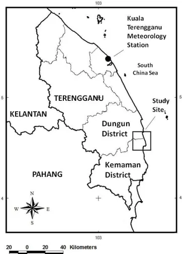
industry [18]. It is also noted that part of the major contribution to the stationary emission sources are from petrochemical plants which are among the 27,000 of the major air pollution in the United States [19]. Historically, petrochemical industry at East Coast of Peninsular Malaysia has started in mid 90‟s [20] and continue to expand since then. The Petrochemical industry area in this region is capable of producing 6.3 million tons per year of various petrochemical products that is equivalent to 50 % of the total Malaysian petrochemical product [21]. From those figures, 4.2 million tons per year or 33% of the national petrochemical products are produced in the State of Terengganu located at Kertih Petrochemical Industry Area (Figure 1). This high productions capacity figure may represent high contribution to air pollution. Geographically, this petrochemical industry located along the coastal zone and very much influenced by North East Monsoon with relatively uniform equator climate throughout the year [6][22]. On top that, this petrochemical industry located within the two main state districts known as Kemaman and Dungun that consist of the second and third largest population after the capital district of Kuala Terengganu [23]. As many sources indicate that air pollution could cause harmful effect to human health, therefore it requires to be controlled [24][25][26]. In Malaysia, this controlled realizes through enforcement of the Environmental Quality Act and Regulation 1974 [27].

Fig. 1. Research location – Kertih, A major petrochemical industry site at North-East of Peninsular Malaysia located

In order to predict the air pollutant, researchers have applied specific tools for specific pollutant emission sources. One of the common tools that being widely used throughout the world is the air dispersion modeling software consist of various models that fit into the research requirement [28]. It is also noted that limited of the predictions using different software models could be specifically recognized as the optimum result due to several factors. One of those are due

to combination of very complex meteorological parameters such as the application of various techniques to estimate surface mixed layer depth above the ground. The various estimation of mixing height techniques has its own advantages that do not guarantee one is above to the other [29]. However, with the above-mentioned limitation, researchers have agreed that the monthly standard of correlation coefficient value of 0.50 and above is considered acceptable [8].

Looking into the scenario above and with the availability of the relevant and acceptable tools, it would be a need to predict on the magnitude of NO2 emitted by the

petrochemical plants at Kertih Industrial Area located North East of Peninsular Malaysia.

II. METHODOLOGY

This paper will utilize the air dispersion modeling known as Industrial Source Complex Short-Term Model (ISCT3). There are four main components which are required in order to simulate and predict on ground concentration of NO2. They

are the meteorological input parameter, point source and NO2

emission estimation, geographical domain set up and finally the verification process through optimization analysis of the meteorological parameters.

A Air Dispersion Modeling

An atmospheric dispersion modeling is a mathematical simulation of the physics and chemistry governing the transport, dispersion and transformation in the atmosphere. The model estimates downwind air pollution concentrations given information about the pollutant emissions and nature of the atmosphere. The model calculates the pollutant concentration using information of the given meteorological, contaminant emission rate and characteristics of the emission source together with the local topography features. The ISCT3 is commonly used air dispersion software among researchers [30][31] and it is recommended by the United States Environmental Agency to perform atmospheric dispersion modeling [32]. The ISCT3 is incorporated with the steady state Gaussian Plume Model and capable of evaluating the pollutant concentration emitted by point sources as follows (Figure 2).

p

o

in

t

so

u

rce

ground

S

ID

E

TO

P

115604-8282 IJET-IJENS @ August 2011 IJENS _{I J E N S}





























2

2

exp

,

,

z y z

y

h

y

u

Q

z

y

x

C









(1)

(at

Where

C =pollutant concentration (ug/m3₎

x =distance downwind from point source (m)

y =cross-wind distance from plumb centerline

(m)

z = vertical distance (m); z = 0 is for

concentration at ground level

Q = contamination emission rate (gm/s)

σy(x) =“cross-wind dispersion coefficient” (m), a

function of x

σz(x) =“vertical dispersion coefficient” (m), a

function of x

u = mean wind velocity (reorient the coordinate

system so the wind always blows in the x

-direction; m·s-1)

h =“stack height” = height above the ground the

pollutant is released (m)

Fig. 2. Steady state Gaussian Plume Model shows formula applied and dispersion of pollutants

This steady state Gaussian Plume Model above utilizes by the ISCT3 may not be an ideal tool to apply under turbulence sea and land breeze condition [28]. As known, the turbulence factors are critical role in determining the pollutant deposition pattern around sources [4]. However, it was noted that ISCT3 being widely used in the United States coastal region, for example at Apalachicola, Daytona, Tampa and West Palm Florida [33] as in need of immediate attention to the pollutants dispersion. Evidence has shown that meteorological database from these locations are available for modeling purposes using the ISCT3 software. The requirements to the input of ISTC3 are the meteorological parameters, point source and NO2 emission estimation and

geographical domain set up are explained accordingly as follows.

B. Meteorological Input Parameter

Hourly meteorological data of year 2008 from Kuala Terengganu Meteorological Station would be processed into the ISCT3 Software. The Kuala Terengganu Meteorological Station located at approximately 95 km north of the study site (Figure 3). Meteorological data from this station is applied in this research since there is no local meteorological station

available at study site. This specific station is selected due to its similarity topography and climate condition with the study site. As an example, both of these sites located at approximately 2 km off the coastal zone which is influenced by sea and land breeze circulation that create turbulent diffusion [1][28]. The Kuala Terengganu Meteorological Station and study site also experience relatively the same atmospheric condition, as Malaysia known to have a uniform climate condition throughout the year at mean temperature ranging between 26 Co to 20 Co [6][23]. Beside the above-mentioned factor, the application of using remote meteorological data is practicality relevant as other researcher has successfully applied the same principle of remote meteorological data, as far as 500 km off the research site [34].

Fig. 3. Remote distance of Kuala Terengganu Meteorological Station north of the study site

The ISCT3 requires two separate meteorological data files in order to execute its programmes; the hourly surface data file (SCRAM MET 144) and daily a.m. and p.m. mixing height file (SCRAM). The SCRAM MET 144 file consists of meteorological parameter which are the ceiling height, wind direction, wind speed, dry bulb temperature and cloud cover with respect to the station number, year month, day and hour concerned. The SCRAM MET 144 file would generate the Wind Rose Plot (WRP) that provides an overview of wind blow direction. The SCRAM file consists of maximum a.m. and p.m. mixing height value. The mixing height is the variation value of the atmosphere height above the ground where the vertical mixing takes place due to mechanical or convection turbulence obtained through the application of the (x,y)

plumb centerline

115604-8282 IJET-IJENS @ August 2011 IJENS _{I J E N S}

Venkatram (1980) formula under stable boundary layer as follows [29].

h = 2300U*1.5 (2)

Where;

h

U

U

Z

Z

The friction velocity is the combination of Von Karman constant (k), wind speed (Uref,), reference height of wind (Zref)

and surface roughness (Zo). The Zo at 0.15 meter was selected

considering the study site topography to be between “Tree Covered” and “Low-density Residential” which is at 0.1 and 0.2 respectively [35]. The Zref at 14 meter refer to the

anemometer height of the Kuala Terengganu Meteorology Station. Combination of these atmospheric elements has been widely implemented previously [36][37][38].

Finally, combination of hourly surface data file (SCRAM MET 144) and daily a.m. and p.m. mixing height file (SCRAM) will generate the hourly MET file. This final meteorological output combine with the point source emission are required to simulate and predict the average on ground NO2

C. Point Source and NO2 Emission Estimation

This paper focuses on the emission estimation of NO2

from point sources emitted by the petrochemical industry. NO2 is the well known pollutant controlled under the

international and local regulatory [6][7]. There are wide range of acceptable techniques of estimating the emission inventory including the source sampling, source emission model, surveying, material balance, emission factors and extrapolation [39][40]. Since data obtained from petrochemical plants are varies, this study will apply the source sampling and material balance techniques in estimating the emission rate of NO2 which consists of 28

points source as follows.

1. Estimation emission rate of NO2 based on actual sampling

data; the conversion of volumetric flow rate of g/m3 to emission rate of g/s. [41][28].

ER (g/s) = C (g/m3) x A (m2) x V (m/s) (3)

Where;

ER = Emission rate pollutant C = Concentration of pollutant

A = Area of point emission based on internal

diameter V = Velocity

2. Estimation emission rate of NO2 based on natural gas flow

rate using material balance techniques; the ultimate fuel analysis [42];

ER (g/s) = Qf (kg/hr) x PCf (%) x (MWp/MWf) x (1000/60 x 60) (4)

Where;

ER = Emission rate pollutant Qf = Fuel flow rate

PCf = Pollutant concentration in fuel N2 = 0.9

%*

MWp = Molecular weight of pollutant emitted (g/g-mole) NO2 = 46

MWf = Molecular weight of pollutant in fuel (g/g-mole) N2 = 28

*[43]

Other point source parameters which compulsory in order to perform atmospheric simulation in this study are including the release height, exit temperature, exit velocity and inside diameter of release point as input into the ISCT3. Simulation result by the ISCT3 will be super-imposed onto the domain set up leads to the overview formation of on ground NO2

distribution contour.

D. Geographical domain set up

The geographical domain set up in this study covers 20 x 20 km2 area surrounding the petrochemical plants with 500 meter each of grid spacing as dummy receptors. The point source location coordinates are identified by matching the longitude and latitude to AutoCAD coordinate. The final part of this study will be the optimization of the meteorological parameter particularly the wind direction. This process is necessary in order to determine the optimum correlation coefficient of the predicted over the actual data of NO2which

lead to the identification of the maximum magnitude value within the set up domain.

E. Optimization and Verification Analysis

The optimization process is performed through wind direction analysis as part of the verification of the predicted over actual NO2 data. This process is performed due to

unavailability of local meteorological at the study site and after careful consideration of the atmospheric and topography similarity of both sites as explained. This technique has been successfully implemented by the local researcher in his recent study to gauge the monthly predicted NO2 against the actual

data from a specific petrochemical plant within the same study site [44].

115604-8282 IJET-IJENS @ August 2011 IJENS _{I J E N S}

increment of 5o rotation. The rotation angle is refined at 1o angle towards the optimum condition. The optimum condition is obtained from the maximum correlation coefficient value obtained from formula defined as follows.

[∑

]

(5)

Where;

A

P

σ

N

III. RESULT AND DISCUSSION

A. The Wind Rose Plot (WRP)

As mentioned, wind condition is one the factor that determines the pollutant distribution. From the WRP generated shows that the majority frequencies of wind directions are blowing from two directions. They are from north-east and south-west directions. The highest wind speed range at 5.40 m/s to 8.49 m/s are blowing from north-east shows that the study site is much influenced by the north-east monsoon (Figure 4). The average wind speed encountered for year 2008 is at 2.08 m/s with 11.18% of those is in calm condition.

Fig. 4. The wind rose plot shows spokes of wind blowing direction measured at Kuala Terengganu Meteorology Station for year 2008 .

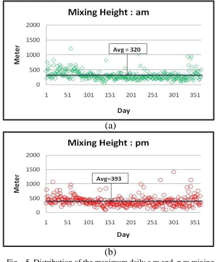
B. The Mixing Height

The application of the Venkatram formula leads to the establishment of the mixing height value at the study location (Figure 5). It is discovered that the minimum and maximum value of the mixing height for year 2008 range from 60 to 1212 meter and 100 to 1414 meter according to a.m. and p.m. period. The average a.m

mixing height is at 320 meter while the average p.m. value is at 393 meter. The application of the Venkatram formula in identifying the mixing height value has proven that it is in line with the traditional theory understood in general where the p.m mixing height is higher than the a.m value mainly due to the influence of

WIND ROSE PLOT

Station #48618 - ,

NORTH

SOUTH

WEST EAST

4% 8%

12% 16%

20%

Wind Speed (m/s) > 11.06 8.49 - 11.06 5.40 - 8.49 3.34 - 5.40 1.80 - 3.34 0.51 - 1.80 UNIT

m/s

DISPLAY

Wind Speed

CALM WINDS

11.18%

MODELER DATE

9/29/2009

COMPANY NAME COMMENTS

WRPLOT View 3.3 by Lakes Environmental Software - www.lakes-environmental.com

PLOT YEAR-DATE-TIME

2008 Jan 1 - Dec 31 Midnight - 11 PM

AVG. WIND SPEED

2.08 m/s

ORIENTATION

Direction (blowing from)

115604-8282 IJET-IJENS @ August 2011 IJENS _{I J E N S}

the surface heat flux generated during the day time is higher than night time.

(a)

(b)

Fig. 5. Distribution of the maximum daily a.m and p.m mixing height for year 2008

C. Point Source Specification and NO2 Emission Estimation

Data gathered and analyzed shows that the NO2

emission rate emitted by 28 point sources range from 0.02 g/s to 8.17 g/s with the average of 2.04 g/s. This estimation of NO2 emission rate obtained through

calculation either from the sampling data flow rate (g/m3) or from natural gas combustion rate (kg/hr) as mentioned on Section II - C. The summary input of the point source specification in the ISCT3 software is summarized as follows.

TABLE I

SUMMARY OF DATA INPUT INTO ISCT3

Min. Max. Avg.

*Emission rate (g/s) 0.02 8.17 2.04

*Release height

(m)

15 87 45.5

*Temperature (oC) 310 600 434

*Exitvelocity(m/s) 4.13 28.00 13.95

*Inside dia.(m) 0.52 3.40 1.46

NO2 flow rate(g/m3)

0.01 0.09 0.04

Natural gas flow rate (kg/hr)

115 1989 743

* Direct input into ISCT3

Finally, combination input of the meteorological data file, point source specification and NO2 emission

estimation into the ISCT3 will generate the predicted on ground concentration of NO2 of which need to be

verified and optimized over the actual data accordingly.

D. Verification and Optimization Analysis

The verification analysis of the predicted on ground concentration of NO2 simulated by the ISCT3 is gauged

to the actual NO2 data obtained accordingly. The initial

ISCT3 simulation of the monthly average shows lower relationship of correlation coefficient value of the predicted against actual NO2 which is at 0.68 (Figure 6).

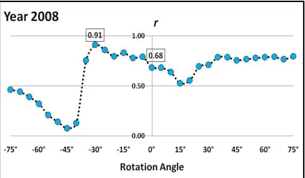
By applying the optimization process through simulation of wind direction at the increment of 5o and finalize at the 1o rotation (Figure 7), the correlation coefficient is discovered improve to 0.91 at 29o angle (Figure 8).

(a)

(b)

Fig. 6. (a- b) Time series comparison of monthly predicted against actual NO2shows low correlation coefficient at „0‟ angle

115604-8282 IJET-IJENS @ August 2011 IJENS _{I J E N S}

Fig. 7. Optimization process throughsimulation of wind direction

(a)

(b)

Fig. 8. (a-b) Time series comparison of monthly predicted against actual NO2shows improve correlation coefficient at the optimum

angle of wind direction

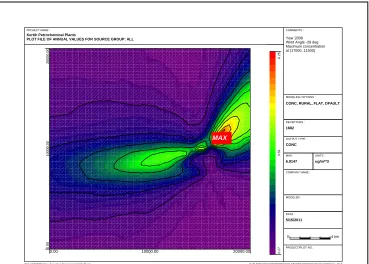
The above optimum condition of the predicted over actual NO2 is applied to simulate the average on ground

distribution of monthly and yearly NO2 surroundings the

petrochemical plants. The distribution contours are used to identify the magnitude of the NO2 distribution

accordingly (Figure 9). From the contours obtained, it is discovered that the maximum on ground concentration of monthly and yearly NO2 is at 13.97 ug/m3 and 6.91

ug/m3 respectively. The yearly value is much below than the WHO guidelines which is at 40 ug/m3 respectively. No benchmarking could be gauged to the monthly value since no guideline is available.

(a)

DATE :

5/15/2011

MODELER : OUTPUT TYPE :

CONC

MODELING OPTIONS :

CONC, RURAL, FLAT, DFAULT

MAX :

13.97428

COMPANY NAME : UNITS :

ug/m**3 MAX

0.00 10000.00 20000.00

200

00.00

0.00

100

00.00

D:\FURTHER\ISCT3PROTOCOL&TESTING\PROISCP.IS\MOH1GALL.PLT ISC-AERMOD View by Lakes Environmental Software

PROJECT NAME :

Kertih Petrochemical Plants

PLOT FILE OF HIGH 1ST HIGH MONTH VALUES FOR SOURCE GROUP: ALL

RECEPTORS :

1682

COMMENTS :

Year 2008 Wind Angle -29 deg Max concentration at (15000, 10000)

PROJECT/PLOT NO. :

13.

97

7.4

1

0.8

6

115604-8282 IJET-IJENS @ August 2011 IJENS _{I J E N S}

(b)

Fig. 9. The distribution contour of NO2 according to monthly (a) and yearly (b) average of year

2008

IV. CONCLUSION

As of the conclusion, this paper has successfully achieved the objective of performing the atmospheric dispersion modeling within the acceptable and much improve correlation coefficient comparing to the research previously conducted [8][30][34]. It is also revealed that the maximum on ground concentration of NO2 is much lower compare to the local and

international guidelines and this value should not pose appreciable risk of harmful effects to human health. This paper also reveals that the application of remote meteorological data is relevant to research site with similar meteorological parameter that leads to a more flexible technique and less cost for future research

.

V. ACKNOWLEDGMENT

The authors are grateful to the Malaysian Meteorological Department and Malaysian Department of Environment for providing data to this study.

REFERENCES

[1] D.Melas, I. C. Ziomas, and. C. S Zerofos, “Boundary Layer Dynamics in an Urban Coastal Environment Sea Breeze Condition,” Atmospheric Environment, vol. 29(24), pp. 3605-3617. 1995.

[2] M. T. Prtenjak, Z. M.Pasaric, M.Orlic, and B.Grisogono, “Rotation of sea/land breezes along the northeastern Adriatic coast,” Annales.Geophysicae, vol.26, pp. 1711–1724. 2008.

[3] A.Venkatram, and R.Paine, “A Model to Estimate Dispersion of Elevated Releases into the Shear-Dominate Boundary Layer,” Atmospheric Environment. vol.19(2), pp.1797 – 1805. 1985. [4] A.A Jennings, and S.J.Kuhlman, “An air pollution transport

teaching module based on GAUSSIAN MODELS 1.1,” Department of Civil Engineering, Case Western Reserve University, Cleveland, Ohio 44106-7201, USA Environmental Modeling & Software , vol.12( 2-3), pp. 151-160. 1997.

[5] G.M. Masters, Air Pollution. In Introduction to Environmental Engineering and Science 2nd _{Edition 1998 International Edition, pp.}

331. Prentice Hall International Inc New Jersey 1998.

[6] ADB, Asia Development Bank and the clean Air Initiatives for Asia Cities (CAI-Asia) Center. Country Synthesis Report Urban air Quality Management – Malaysia. 2006.

[7] DOE. Department of Environment Malaysia. A guide to Air Pollution Index (API) in Malaysia 2000.

[8] A.Karppinen, J. Kukkonen, T. ElolaKhde, M. Konttinen and T.Koskentalo T. “ A modelling system for predicting urban air pollution: comparison of model predictions with the data of an urban measurement network in Helsinki,” Atmospheric Environment, vol. 34, pp. 3735- 3743. 2000.

[9] M. Neuberger, G. Michael, M.G. Schimek, F. Horak, H. Moshammer, M. Kundi, T. Frischer, B. Gomiscek, H. Puxbaum and H. Hauck, “Acute effects of particulate matter on respiratory diseases, symptoms and functions:: epidemiological results of the

DATE :

5/15/2011

MODELER : OUTPUT TYPE :

CONC

MODELING OPTIONS :

CONC, RURAL, FLAT, DFAULT

MAX :

6.9147

COMPANY NAME : UNITS :

ug/m**3

MAX

0.00 10000.00 20000.00

200

00.00

0.00

100

00.00

D:\FURTHER\ISCT3PROTOCOL&TESTING\PROISCP.IS\AN00GALL.PLT ISC-AERMOD View by Lakes Environmental Software

PROJECT NAME :

Kertih Petrochemical Plants

PLOT FILE OF ANNUAL VALUES FOR SOURCE GROUP: ALL

RECEPTORS :

1682

COMMENTS :

Year 2008 Wind Angle -29 deg Maximum concentration at (17000, 11500)

PROJECT/PLOT NO. :

6.2

5

3.5

9

0.2

7

115604-8282 IJET-IJENS @ August 2011 IJENS _{I J E N S}

Austrian Project on Health Effects of Particulate Matter (AUPHEP),” Atmospheric Environment, vol. 38(24), pp.3971-3981. 2004

[10] Scoggins, A., Kjellstrom, T., Fisher, G., Connor, J. and Gimson, N., “Spatial analysis of annual air pollution exposure and mortality,” Science of The Total Environment, vol. 321(1-3), pp.71-85. 5 April 2004

[11] P.Paatero, P. Aalto, S. Picciotto, T. Bellander, G. Castaño, G. Cattani, J. Josef Cyrys, M.Markku Kulmala, T. Timo Lanki, F.Fredrik Nyberg, “Estimating time series of aerosol particle number concentrations in the five HEAPSS cities on the basis of measured air pollution and meteorological variables,” Atmospheric Environment, vol. 39(12), pp. 2261-2273. 2005

[12] C.M.Wong, C.Q. Ou, T.Q. Thach, Y.K. Chau, K.P. Chan, S.Y.Ho, R.Y. Chung, T.H.Lam and A.J.Hedley, “Does regular exercise protect against air pollution-associated mortality?,” Preventive Medicine, In Press, Corrected Proof, Available online 8 January 2007.

[13] R. Beelen, G.Hoek, P. Fischer, P.A.V.D. Brandt, B. and Brunekreef, “Estimated long-term outdoor air pollution concentrations in a cohort study,” Atmospheric Environment, vol.41(7), pp. 1343-1358. March 2007

[14] Air Quality Data Report, Colorado Department of Public Health and Environment, 2007

[15] Dark, T., Auckland J. and White J. Fuel. The John Zink Combustion Handbook. John Zink Company LLC. ISBN Number 0-8493-2337-1, 2001, pp.157-188

[16] GCM, Gulf Coast Midwest Energy Partners, LLC. Natural Gas Basics, 2008.

[17] K. E. Zanganeh, A. Shafeen, and k. Thambimuthu , “A Comparative study of Refinery Fuel Oxy-Fuel Combustion Options for CO2 Capture Using Simulation Process Data,” Journal

Greenhouse Control Technologies,vol.II, pp.1117-1123. 2005. [18] H. Akimoto and H Narita, “Distribution of SO2, NOx and CO2

emissions from fuel combustion and industrial activities in Asia with 1° × 1° resolution,”. Atmospheric Environment, vol. 28(2), pp.213-225. January 1994.

[19] T. Tietenberg, Stationary Source Local Air Pollution In Environmental and Natural Resource Economic, Addison Wesley, Pearson Education Inc ISBN 0-201-77027-X. 2005, pp 366 [20] PETRONAS Annual Report 2006

[21] MPA, Malaysian Petrochemicals Association. Asia Petrochemical Industry Conference 2003 Country Report – Malaysia

[22] MMD, Malaysian Meteorological Department, General Climate of Malaysia, 2010

[23] RSNT, Rancangan Struktur Negeri Terengganu (Structure Program State of Terengganu 2005 -2020), 2004

[24] N.D. Nevers, Air Pollution Effects. In Air Pollution Control Engineering. McGraw-Hill ISBN 0-07-061397-4, 1995, pp. 11-31 [25] DOSH, Department of Occupational Safety and Health Malaysia.

Assessment of the Health Risks Arising From The Use of Hazardous Chemicals in the Workplace – A Manual of Recommended Practice 2nd _{Edition. 2000.}

[26] R.T. Wright and B.J. Nebel, Atmospheric Pollution. In Environmental Science, Toward a Sustainable Future. New Jersey: Pearson Education. 2002, pp 541-546

[27] EQA, Environmental Quality Act and Regulations, Laws of Malaysia ACT 127 April 2006 pp. 107-125. MDC Publishers Sdn Bhd ISBN 967-70-0820-X

[28] J. Bluett , N. Gimson, G. Fisher, C. Heydenrych, T. Freeman and J. Godfrey. Good Practice Guide for Atmospheric Dispersion Modeling, 2004.

[29] A. Baklanov, S.M. Joffre, M. Piringer, M. Deserti, D.R. Middleton, M. Tombrou, A. Karppinen, S. Emeis, V. Prior, M.W. Rotach, G. Bonafè, K. Baumann-Stanzer and A. Kuchin. DMi Ministry of Transport and Energy (Copenhagen), Scientific Report 06-06 Towards estimating the mixing height in urban areas. Recent

experimental and modeling results from the COST-715 Action and FUMAPEX project, 2006.

[30] D. Pimpisut, W. Jinsart and M.A. Hooper, “Modeling of the BTX Species Based on an Emission Inventory of Sources at the Map Ta Phut Industrial Estate in Thailand,” Science Asi, vol.31, pp.102-112, 2005.

[31] J.G. Brody, D.J. Vorhees, S.J. Melly, S.R. Swedis, P. J. Drivas and R.A. Rudel, 2002. “Using GIS and Historical Records to Reconstruct Residential Exposure to Large-Scale Pesticide Application,” Journal of Exposure Analysis and Environmental Epidemiology, vol.12, pp 64–80, 2002.

[32] EPA. U.S., Environmental Protection Agency, U S. Air Quality Management Online Portal Air Quality Modeling - Resources:

Publications and Reports, 2006.Available:

http://www.epa.gov/air/aqmportal/management/links/modeling_res ources_pub.htm

[33] EPA U.S., Environmental Protection Agency, U S. Technology Transfer Network Support Center for Regulatory Atmospheric Modeling SCRAM Surface Meteorological Archived Data 1984

-1992, 2006. Available:

http://www.epa.gov/scram001/surfacemetdata.htm

[34] T. Elbir, “Comparison of model predictions with the data of an urban air quality monitoring network in Izmir, Turkey,” Atmospheric Environment, vol.37, pp. 2149–215, 2003.

[35] G. J. McRae, W.R Goodin and J.H. Seinfeld, “Development of a second-generation mathematical model for urban air pollution. Model formulation,” Atmospheric Environment, vol.16(4), pp. 679-696, 1982.

[36] Guan Dexin, Zhu Tingyao, Han Shijie, “Friction Velocity U* and

Roughness Length Z0 of Atmospheric Surface Boundary Layer in

Sparse-tree Land 1,” Journal of Forestry Research. vol.10(4), pp. 119-202, 1999.

[37] O.Fatogoma and R.B. Jacko, “A Model to Estimate Mixing Height and its Effects on Ozone Modeling,” Atmospheric Environment, vol. 36, pp. 3699–3708, 2002.

[38] S.A, Hsu, “Estimating Overwater Friction Velocity and Exponent of Power-Law Wind Profile from Gust Factor during Storm,” Journal of Waterway, Port, Coastal, and Ocean Engineering. vol.129(4), pp. 174–177, 2003.

[39] MEIPM. Volume III, Mexico Emissions Inventory Program Manual 1996, Volume III – Basic Emission Estimating Techniques, DCN 96-670-017-01, RCN 670-017-20-04. Western Governers‟ Association Denver, Colorado and Radian International Sacramento, California, 1996.

[40] CCPA, Canadian Chemical Producers‟ Association. Source Characterization Guidelines. Primary Particulate Matter and Particulate Precursor Emission Estimation Methodologies for Chemical Production Facilities, 2004.

[41] L. Jesse, L. Cristiane and L.A. Johnson, User‟s Guide ISC-AERMOND View, Lakes Environmental, 2000, pp 4-9.

[42] MEIPM. Volume IV, Mexico Emissions Inventory Program Manual 1996, Volume IV– Point Source Inventory Development, DCN 96-017-21-05, RCN 670-017-20-04. Western Governers‟ Association Denver, Colorado and Radian International Sacramento, California. 1996.

[43] EPA U.S., Environmental Protection Agency, U S. Preliminary Characterization Study. Traditional Fuels and Key Derivatives - Advanced Notice of Proposed Rule Making, Identification of Nonhazardous Material That Are Solid Waste, 2010.

[44] M.H. Ibrahim, A.M. Abdullah, J. Juliana and L.K. Chng, Sensitivity Analysis of Wind Rotation in Determining the Correlation of Pollutant Concentration (NO2) with Location in