Determining the optimal feature for two classes
Motor-Imagery Brain-Computer Interface
(L/R-MI-BCI) systems in different binary classifiers
Nibras Abo Alzahab
1, Hassan Alimam
2, MHD Shafik Alnahhas
3, Ali Alarja
4and Zuheir Marmar
5.
1. Biomedical Engineer, Biomedical Engineering Department, Faculty of Mechanical and Electrical Engineering, DamascusUniversity,
2. Teaching Assistant, Mechanical Design Engineering Department, Faculty of Mechanical and Electrical Engineering, Damascus University,
[email protected], [email protected]
3. Undergraduate Final Year Student, Biomedical Engineering Department, Faculty of Mechanical and Electrical Engineering, Damascus University,
4. Biomedical Engineer, Biomedical Engineering Department, Faculty of Mechanical and Electrical Engineering, Damascus University,
5. Professor, Biomedical Engineering Department, Faculty of Mechanical and Electrical Engineering, Damascus University, [email protected]
Abstract--Day-by-day, artificial intelligence becomes more and more important in the field of healthcare. One important application is Brain-Computer Interface (BCI) which has many advances in enhancing the life quality of patients who suffers from paralysis for a reason or another. Motor-Imaginary BCI (MI-BCI) is mostly used to control robotics and mechatronic systems, for example robotic arms, orthosis, prothesis and exoskeletons. This research evaluates the effect of different features on classification process of EEG signal in MI-BCI systems. In this study, five healthy subjects performed trailing imagery in order to acquire EEG signal dataset. Five feature groups were extracted (Power Spectral Density (PSD), Amplitude mean (AM), Standard Deviation (STD), Shannon Entropy (SE) and Differential Entropy (DE)) from EEG signal in MI-BCI of five different subjects. The features groups are classified using five classification technique "ANN, Decision tree, LDA, SVM, and KNN. The influence of features groups in classification performance was compared separately according to three classifier criteria (Accuracy, Precision and MCC). One-way ANOVA test was used to compare influence of features groups in classification performance. For classification accuracy and precision, significant differences were obtained in SVM and ANN classifiers for pairs of features which is fairly supported by the experimental and statistical data. The results of the research show that Power Spectral Density (PSD) feature shows great ability to describe EEG signal in MI-BCI field and considered as an effective feature in binary classifiers. Additionally, Differential Entropy (DE) is considered as a promising feature to be used in MI-BCI field. The results of this study will be used for developing robots, bio-mechanical, and bio-mechatronic systems in ACIA Lab. Index Term-- Electroencephalography (EEG), G-tech, Artificial Intelligent (AI), Motor Imaginary Brain Computer Interface (MI-BCI), Feature extraction, Binary-Classification, MATLAB, SPSS, One-way ANOVA, Mathew Correlation Coefficient (MCC).
1- INTRODUCTION
Artificial intelligence (AI) is becoming more and more important in every aspect of life, for example industrial [1] and medical applications. One of the most promising medical applications of AI is Brain Computer Interface (BCI) [2]. Brain-Computer Interface (BCI) system is a communication system that depends on abnormal brain activity. In other words, without depending on peripheral muscular activity. This definition was shaped in the first international meeting in 2000 which was sponsored by international the National Center for Medical Rehabilitation Research of the National Institute of Child Health and Human Development of the National Institutes of Health [3].
Many efforts were being contributing to developing Brain-Computer Interface (BCI) systems since then. Mason and Birch in 2003 proposed a general framework for Brain– Computer Interface design [4]. The proposed model consists of nine components namely: the user, electrodes, amplification, feature extraction, feature translation, control interface Device Controller, Device and Operating environment. However, this framework was modified through time to be as it is shown in Solis-Escalante's thesis [5] illustrated in Fig. 1. The upgraded scheme uses machine learning in two stages, Feature extraction and classification, to translate the EEG signal from the world of signal processing into the world of control (feedback application).
F. Lotte et.al. in 2007 published a research paper to review
the algorithms used in classifying the
networks, nearest neighbor classifiers and combinations of classifiers. In the end of the review, they provided a guideline for researcher to choose the most suitable classification algorithm for their research [6].
Herman et. al. in 2008 conducted a comparative analysis between the number of features. The comparison, mainly, depends on classifier accuracy (CA). In addition, three classification algorithms were applied namely: Linear discriminant analysis (LDA), regularized Fischer discriminant (RFD) and support vector machine (SVM) with linear and nonlinear kernels. As a result, Power Spectral Density (PSD) was the most appropriate feature [7].
ZHAO et. al in 2009 depended in their research, in the field Motor Imaginary Brain-Computer Interface (MI-BCI), on
how the duration of event-related
desynchronization/synchronization (ERD/ERS) could be modulated and used to control a car in the 3D virtual reality environment. They classified the MI-BCI into four classes: left, right, foot (speed up) and no order. The proposed approach is able to drive smoothly a virtual car [8].
Shan et. al. in 2015 provided a method to select the optimal channel for classifying EEG signal in the field of Motor Imaginary Brain-Computer Interface (MI-BCI). Each feature they used in their research was the average of Hilbert transform, which reflect the power, of each sub-band in the range from 5 Hz to 35 Hz over the time of the trail. The classifier used was multiclass Support Vector Machine (SVM). The proposed method shows ability to effectively classifying multi-class motor imagery patterns [9].
Shang-Lin Wu in 2016developed an innovative method with swarm-optimized fuzzy integral to classify MI-BCI system based on EEG signals into two classes, in order to control the movement of a robotic arm. They used single LDA, Conventional Methods and Fuzzy Fusion with Sugeno Integral and Choquet integral Classification algorithms. The best classification accuracy was achieved using Choquet integral with particle swarm optimization [10].
Alansari, M., Kamel, M et. al.in 2018 developed an enhancement method for BCI systems. The developed
method depends on wavelet-based feature extraction using different sub bands of EEG signal. The research tested different families, lengths and number of decomposition levels. The results show that the proposed optimization process outperformed other previous methods [11].
Datta, A., & Chatterjee, R. in 2019 presented three types of feature extraction methods namely: Wavelet-based Energy and Entropy (EngEnt), Bandpower (B P), and Adaptive Autoregressive (AAR). Additionally, they combined the extracted feature with various classification algorithms namely: Support Vector Machine (SVM), K-Nearest Neighbors (K-NN) and Naive Bayes (NB). As the research results, EngEnt is the most suitable feature extraction method and K-NN is most stable classification algorithm [12].
This paper is considered as a step forward in our project conducted in ACIA Lab (Automatic Control and Industrial Automation Lab), Damascus University towards building bio-controlled pneumatic bio-robotics [13]. The goal of the research is to study various binary classifiers response to different features extracted from EEG signals in MI-BCI field. Therefore, the results of this research will be used to control pneumatic bio-robotics, orthosis and prothesis in specific. This methodology of the paper is consisting of four main parts. Firstly, describing the data used in this research which was provided by the Dr. Cichocki's Lab [14]. Secondly, reviewing five features extracted from EEG signals namely: Power Spectral Density (PSD), Standard Deviation (STD), Amplitude Mean (AM), Shannon Entropy (SE) and Differential Entropy (DE). The review includes theoretical description, mathematical equations and programing code for each feature. Thirdly, a short description of each classification algorithm. Finally, the experimental work and classification performance criteria. Afterwards, statistical analysis of the classification performance criteria is described profoundly and explained with a flow chart. In the end, the results of the statistical analysis was mentioned and discussed. Table VIII and Table IX shows the used Abbreviations and symbols respectively. The overall architecture of the research is shown in Fig 2.
Fig. 2 Overall architecture of the research. 2-METHODOLOGY
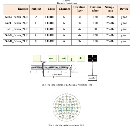
2.1 - Datasets Description:
Datasets are provided by the Prof. Cichocki’s Lab (Lab. for Advanced Brain Signal Processing), BSI, RIKEN in collaboration with Prof. Liqing Zhang in Shanghai Jiao Tong University [14].
Datasets recording:
At the beginning of a trail, the subject was sitting in front of a blank computer screen. Two seconds after the trail started, a cue appeared on the screen as an arrow, left arrow for imagining left hand movement and right arrow for imagining right hand movement. The cue duration is represented in Table. 1 in the duration column. g.tec (g.USBamp) was used to record the electroencephalography
Table I Datasets description
Dataset Subject Class Channel Duration
(sec)
Trialsnu mber
Sample
rate Device
SubA_6chan_2LR A LH/RH 6 3s 130 256Hz g.tec
SubC_6chan_2LR C LH/RH 6 3s 071 256Hz g.tec
SubF_6chan_2LR F LH/RH 6 4s 80 256Hz g.tec
SubG_6chan_2LR G LH/RH 6 4s 120 256Hz g.tec
SubH_6chan_2LR H LH/RH 6 3s 150 256Hz g.tec
Fig.3.The time scheme of EEG signal recording [14].
2.2 Feature Extraction
We aimed to extract five features in order to determine the optimal feature to be applied in MI-BCI systems. The five features are: Power Spectral Density (PSD), Standard Deviation (STD), Amplitude Mean (AM), Shannon Entropy (SE) and Differential Entropy (DE).
2.2.1 Power Spectral Density:
The power spectral density (PSD) could be estimated using Welch method [9] that depends on Fourier Transformation. As shown in Fig. 5, Welch's method divides the signal into 𝐾 overlapped segment 𝑋(1), … , 𝑋(𝑗); 𝑗 = 0, … , 𝐿 − 1 where each segment length is 𝐿. We take the finite Fourier Transformation of the sequences 𝑋1(𝑗)𝑊(𝑗), … , 𝑋𝐾𝑊(𝑗), where 𝑊(𝑗) is a selected data window shown in equation (1). Thus, 𝐴1, … , 𝐴𝑘 are the finite Fourier Transformation sequences given in
equation (2):
𝑊(𝑗) = 1 − (𝑗−
𝐿−1 2 𝐿+1 2
)
2
(1) [15]
𝐴𝑘(𝑛) =1𝐿∑𝐿−1𝑗=0𝑋𝑘𝑊(𝑗)𝑒−2𝑘𝑖𝑗𝑛/𝐿 (2) [15]
Where 𝑖 = √−1.
The 𝐾 modified periodogram is obtained by equation (3):
𝐼𝑘(𝑓𝑛) =𝑈𝐿|𝐴𝑘(𝑛)|2; 𝑘 = 1,2, … , 𝐾 (3) [15]
Where
𝑓𝑛=𝑛𝐿; 𝑛 = 0, … ,𝐿2 (4) [15]
And
𝑈 =1𝐿∑𝐿−1𝑊2(𝑗)
𝑗=0 (5) [915
Finally, the average of the periodograms represents the estimated Power Spectral Density (PSD), equation (6):
𝑷̂(𝒇𝒏) =𝟏𝑲∑𝑲𝒌=𝟏𝑰𝒌(𝒇𝒏) (6) [15]
Fig.5. The overlapped segments in Welch's method [6].
This feature was extracted using MATLAB code:
psd_welch(j,i)= sum(pwelch(EEGDATA(j,:,i)))/length(EEGDATA(j,:,i));
Where pwelch is the function that extracts the PSD, psd_welch of a discrete-time signal, EEGDATA, using Welch's averaged, modified periodogram method.
2.2.2 Amplitude Mean:
The signal’s amplitude mean is considered as a time-domain feature. Additionally, it is simple and easy to be extracted which make it computationally effective. However, since it gives information about the shape of the signal, it is difficult to differentiate between the signal of the right-hand movement and the signal of the left-hand movement [29].
Amplitude mean depends on finding the average value of voltage of the EEG signal according to equation (7).
𝒙̅ =∑𝑵𝒏=𝟏𝒙(𝒏)
𝑵 (7) [18]
This feature was extracted using MATLAB code:
Mean(j,i)=mean(EEGDATA(j,:,i));
2.2.3 Standard Deviation:
Standard deviation represents a statistically description of EEG signal in BCI systems [17]. It represents the distance between each sample, of the signal, from the amplitude mean value. Consequently, it can describe the signal more efficient than amplitude mean does. In other words, standard deviation could be used as feature with acceptable accuracy.
The Standard deviation (𝜎) (STD) feature was extracted by applying the statistical equation of the STD, represented in equations (8), over the EEG signal:
𝝈 = √∑𝑵𝒏=𝟏(𝒙(𝒏)−𝒙̅)𝟐
This feature was extracted using MATLAB code:
Std(j,i)=std(EEGDATA(j,:,i));
2.2.4 Shannon Entropy:
Any signal can be decomposed into set of functions (signal's coefficients) by using Wavelet transformation. Therefore, Shannon Entropy (SE) feature was extracted depending on wavelet transformation. The wavelet transformation uses families of functions generated from a basic signal called the mother signal, which is shifted and dilated according to the original signal, called the wavelet [19, 20]. Equation (8) represents the continuous wavelet transformation (CWT):
𝑊(𝑎, 𝜏) = ∫−∞+∞𝑥(𝑡)Ψ̅̅̅̅̅a,𝜏 (8) [19]
Where 𝑎 is the scaling factor, 𝜏 is the shifting factor and Ψ𝑎,𝜏 is the mother wavelet. The mother wavelet is given in equation (9):
Ψ𝑎,𝜏(𝑡) =|√𝑎|1 Ψ (𝑡−𝜏𝑎 ) (9) [21]
There are many wavelet families such as Daubechies, Symlets, Coiflets, Morlet, Mexican hat, and Meyer wavelets . However, Symlets wavelet exhibits the highest compatibilities with EEG signals [22]. Fig. 6 represents the wavelet families.
Fig.6. Wavelet Families (Modified from [23]).
After the signal was decomposed into a number of coefficients, The Energy 𝐸𝑖 of each coefficient was computed as the mean
of squared coefficients. By summing the energies of all coefficients, Total energy 𝐸𝑡𝑜𝑡 was calculated. Afterwards, the ration
between the energy of each coefficient 𝐸𝑖 and total energy equals to the relative wavelet energy 𝑃𝑖 [19, 24], as shown in
equation (10):
𝑃𝑖=𝐸𝐸𝑖
𝑡𝑜𝑡 (10) [1824
Two entropy features are used in this research namely: Log energy entropy, Threshold entropy and Shannon entropy, given in equation (11), (12) and (13) respectively:
𝐸𝑇(𝑠𝑖) {10𝑒𝑙𝑠𝑒𝑤ℎ𝑒𝑟𝑒|𝑃𝑖|>𝑝 (12) [24]
𝑬𝑺𝒉(𝒔) = ∑ 𝑷𝒊 𝒊𝟐. 𝐥𝐨𝐠 (𝑷𝒊𝟐) (13) [24]
Where 𝑝 is the threshold.
Shannon entropy feature was extracted using MATLAB code:
EEG=EEGDATA(j,:,i);
[c,l] = wavedec(EEG,5,'sym3');
[thr,sorh,keepapp]=ddencmp('den','wv',EEG);
EEG2=wdencmp('gbl',c,l,'sym3',5,thr,sorh,keepapp);
Eshannon(i,j)=wentropy(EEG2,'shannon');
Where wavedec, ddencmpandwdencmpreturns wavelet transformation with Symlet-5 as a mother wavelet. And wentropyreturns Shannon Entropy.
2.2.5 Differential Entropy:
Another good feature used to describe the hidden information in EEG signals is Differential Entropy (DE) [26, 27]. DE measures the complexity of a continuous random variable and it is calculated by using equation (14)
ℎ(𝑋) = − ∫ 𝑓(𝑥) log(𝑓(𝑥)) 𝑑𝑥𝑋 (14) [26]
where 𝑋 is a random variable, 𝑓(𝑥) is the probability density function of 𝑋.
It was proven in [26] that EEG signal is subject to the Gaussian distribution 𝑁(µ, 𝜎2), in a series of sub-bands after 2Hz step-band-pass filtering in range from 2Hz to 44Hz. Afterwards, Kolmogorov-Smirnov test verifies that EEG signals meets Gaussian distribution with probability more than 90%. Therefore, its differential entropy, in a fixed frequency band 𝑖, can be calculated by using equation (15)
ℎ(𝑋)=∫ 1
√2𝜋𝜎2𝑒 (𝑥−𝜇)2
2𝜎2 log ( 1
√2𝜋𝜎2𝑒 (𝑥−𝜇)2
2𝜎2 ) 𝑑𝑥 =1
2log (2𝜋𝑒𝜎 2)
𝑋 (15) [25]
hence,
𝒉𝒊(𝑿) =𝟏𝟐𝐥𝐨𝐠 (𝟐𝝅𝒆𝝈𝒊𝟐) (16) [25]
Where ℎ𝑖 and 𝜎𝑖2 denote the differential entropy of the corresponding EEG signal in frequency band 𝑖 and the signal variance,
respectively, in equation (16).
This feature was extracted using MATLAB code, simply by applying the equation 15.:
De(j,i)=0.5*log(2*pi*exp(1)*var(EEGDATA(j,:,i)));
2.3 Classification Algorithms:
In this section, the five applied classification algorithms are briefly discussed namely: Neural Networks (NN), Decision Tree, Linear Distribution Analysis (LDA), Support Victor Machine (SVM) and K-nearest Neighbor (K-NN).
2.3.1 Neural Networks:
boundaries, classify any number of classes and flexible. However, the architecture of the neural network, number of layers and number of neurons in each layer, should be carefully selected [7, 28].
2.3.2 Decision Tree:
A decision tree represents a decision procedure to determine the class of a given input. Its simplicity, flexibility and computational efficiency offers substantial advantages for the classification stage. However, its low accuracy is the major drawback of decision tree [29, 30].
2.3.3 Linear Distribution Analysis (LDA):
LDA, also known as Fisher’s linear discriminant (FLD), is a linear classifier that determine the optimal hyperplane (a point in 1-D space, a Line in 2-D space and a surface in 3-D space) to classify the data into two classes. It is optimal to be applied when the data has an equal covariance matrix and its distribution is Gaussian. LDA shows success in great number of BCI applications like MI-BCI [30] and P300 Speller [32] due to its simplicity and its very low computational requirements. However, its main drawback is its linearity which results unpleasant outcomes when dealing with complex nonlinear Data [7, 19, 32].
2.3.4 Support Victor Machine (SVM)
As LDA, SVM uses a hyperplane to separate the data into two classes but it depends on maximizing the distance, which known as the margin, between the hyperplane and the data points. Basically, SVM classifiers are linear but with a slight increase of its complexity it can produce a nonlinear decision boundary. Despite the fact that SVM classifiers has worthful advantages, it suffers from low speed of execution [7, 19, 32].
2.3.5 K-nearest Neighbor (K-NN)
K-nearest Neighbor is a very simple classifier. It depends on determining the classes of K-nearest Neighbor of an instance. Then, the class of the instance is the same class of the majority of its neighbors [7].
Applying ANN classification depends on “Pattern Recognition and Classification tool (nprtool)” MATLAB Built-in app. And for Decision Tree, LDA, SVM and K-NN applied by using “Classification Learner” MATLAB Built-in app.
2.4 Experimental work:
Each feature was extracted from six EEG channels (C3, Cp3, C4, Cp4, Cz and Cpz) and was used to train classification models, each classification algorithm used to train a model, which mean 25 models for each feature-classifier pair. This procedure was repeated for the five subjects, overall 125 classification model represents the feature-classifier pairs.
The method used to train and validate each model is 10-folds cross validation, resulting of a confusion matrix for each model. The resulted confusion matrices were used to calculate the performance criteria (performance metrics) which are Classifier Accuracy (𝐴𝐶𝐶), Classifier Prescient which, AKA Positive Predicted Value (𝑃𝑃𝑉) and Matthews Correlation Coefficient (MCC), presented in equations (17), (18) and (20), respectively. The structure of the confusion matrix is illustrated in Table. II.
𝐴𝐶𝐶 =𝑇𝑃+𝑇𝑁+𝐹𝑃+𝐹𝑁𝑇𝑃+𝑇𝑁 (17) [33]
𝑃𝑃𝑉 =𝑇𝑃+𝐹𝑃𝑇𝑃 (18) [33]
Table II
The structure of Confusion Matrix [29] True Condition
Total Population
Condition Positive Condition
Negative 𝐴𝐶𝐶 =
Σ 𝑇𝑃 + Σ 𝑇𝑁 Σ 𝐴𝑙𝑙 𝑃𝑜𝑝𝑢𝑙𝑎𝑡𝑖𝑜𝑛 Predict
ed Condit
ion
Predicted Condition Positive
True Positive (TP) False Positive (FP)
𝑃𝑃𝑉
= Σ 𝑇𝑃
Σ 𝑃𝑟𝑒𝑑𝑖𝑐𝑡𝑒𝑑 𝑐𝑜𝑛𝑑𝑖𝑡𝑖𝑜𝑛 𝑝𝑜𝑠𝑖𝑡𝑖𝑣𝑒 Predicted
Condition Negative
False Negative (FN) True Negative (TN)
3-STATISTICAL ANALYSIS
According to parametric statistical method [34, 35, 36], the performance of binary classifier was determined by comparing whether the optimal mean effect of different data collected from five subjects as a training MI-BCI feature have a significant difference, or otherwise this training feature samples (trails) are not differ on each other, which mean that average values of training feature samples are similar. Therefore, five features groups “statistically” were extracted (Power Spectral Density (PSD), Amplitude mean (AM), Standard Deviation (STD), Shannon Entropy (SE) and Differential Entropy (DE)) from EEG signal in MI-BCI of five different subjects; five samples from five subjects were represented as independent samples for each features group. The influence of the features groups in classification performance was compared separately according to two classifier criteria (Performance metrics), namely: Accuracy and Precision. Therefore, to determine classifier learning effects over features groups, classification performance differences between the different features groups were compared using one-way ANOVA (parametric analysis of variances) separately for Accuracy and Precision. The features (PSD, AM, STD, SE and DE) were considered as several independent variables and dependent variables as accuracy and precision separately.
The reliability of applying parametric test was detected by checking that individual classification performance data was normally distributed. Therefore, Shapiro-Wilk and Kolmogorov-Smirnoff statistical test were used at 0.05 significance levels to avoid whether the normality assumption was in doubt. However, these statistical tests are very sensitive when the sample size in each feature group was less than 20 samples (df = 5 < 20). Consequently, in each feature group sample size was consisted of five subjects which was less than critical sample size twenty (df = 5 < 20), therefore non-normality is less likely to be checked by statistical test only "Shapiro-Wilk". However, the test of normality will be carried out and the testing errors for normality will be detected by creating the unstandardized residuals for each dependant variables “classification performance criteria” and testing the normality for the residuals. When normality was reached, ANOVA parametric test was performed using two assumptions. First assumption, which was evaluated at significance level (a = 0.05) by t-test "Levene's test" to
ensure that homogeneity of variances between feature-groups, has not been violated. Second assumption was discussed depending on the results of Levene's test and ANOVA test in order to determine whether a significant F ratio was obtained, therefore, to reject the null hypothesis and accept the alternative hypothesis, which states that classification performance criteria is different across features groups at significance level (a = 0.05). When the second assumption was reached significance (p< 0.05), multiple comparisons were performed using subsequent post-hoc t-tests, firstly, to determine difference between groups and, secondly, to compare between which features a significant difference “in performance criteria” can be conducted. Afterwards, when the first assumption was reached significance (p> 0.05), and equal variances were assumed, Tukey HSD test will be applied. However, Games-Howell post hoc test will be performed when first assumption was rejected and unequal variances were assumed. Significant difference will be considered by post-hoc t-test when the p-value was below 0.05. Fig.7 demonstrates a flow chart of the statistical analysis. Statistical analysis was performed using statistical package for the social science SPSS 17.0.
Mathew's correlation coefficient:
In order to determine the significant influence of features group on the generalization capability of classification system, Mathew's correlation coefficient (MCC) was calculated besides the popular performance criteria (Accuracy and Precision). It is considered as a measurement factor in which the quality of binary classification can be evaluated significantly under the MCC values range from (–1 ≤ MCC ≤ 1). MCC value can be calculated by means of confusion matrix based on the correlation between outcomes and predicted binary classifications [34, 37]. The MCC can be calculated directly using the following equation (19).
The possible perfect prediction was achieved when the MCC value reaches to +1, random prediction results represent with zero value. But disarrangement between prediction and observation indicates worst prediction represent when MCC reaches -1.
4–RESULTS AND DISCUSSION
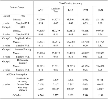
mean of accuracy of 77.33 % was obtained with the ANN classifier for differential entropy feature. Whereas, the smallest 51.95% was obtained with the decision tree classifier for amplitued mean feature. For accuracy means values obtained by ANN, Decision Tree, LDA, SVM, and KNN classifiers, There are No evidance that individual features data is not normally distributed. p values for the Shapiro-Wilk test is more than 0.05 (p>.05) suggesting that the data is normally distributed. Also p values for residuals are greater than 0.05 (p>.05) which indicats the normality for the residuals. Assumption for homogeneity of variance are checked by Levene's test. In ANN, Decision tree, and LDA classifiers, Levene's test for homogeneity of variances is not significant (p>.05) and therefore we can be confident that the population variances for accuracy data are approximately equal. In SVM and KNN classifiers, Levene's test resulted in significant results (SVM: p-value = 0.004;
KNN: p-value = 0.045) and therefore the homogeneity of variance assumption has been violated (p< .05). The ANOVA test was significant (p< .05) to test feature effect on classification accuracy for ANN and SVM classifiers. So effect resulted in significant results for classification accuracy (SVM: F(4, 20) = 3.944, p = 0.016 < 0.05; ANN:
Table V shows the mean of classification precision of different classifiers depending on features groups. The minimum classification precision in the SVM, Decision tree and KNN classifier was obtained for Amplitude mean and PSD. It was 51.3% in Decision tree for Amplitude mean, 53.8% in SVM for Amplitude mean and 52.5% in KNN for PSD. However, for all features "PSD, STD, AM, SE, and DE", the maximum mean precision has attained the highset avarage in ANN classification algorithm. Table IV demonstrates the following means of precision related to ANN classifier: 76.7% for Shannon entropy, 76.5% for differential entropy, 75.5% for STD, 74.9 for PSD, and 64.4 for Amplitude mean (Table IV).
During the first assumption of statistical analyses, p values for individual feature data in classification precision indicate that there is strong evidence of normality for each feature group. This is clearly represented at p values for the Shapiro-Wilk test, which is more than 0.05 (p>.05) suggesting that the data is normally distributed.
Also p values for residuals are greater than 0.05 (p>.05) which indicate the normality for the residuals. Furthermore, the equality of variances for precision data depending on Levene's test was analyzed. The p value obtained was 0.162, 0.756, and 0.072 for ANN, LDA, and KNN classifiers, respectively (Table IV), therefore threre is no evidence to doubt assumption of equal variances for precision data. Whereas other precision data for SVM and Decision Tree classifiers have strong evidence to violate homogeinety of variance assumption (p-values < .05) (Table IV). The ANOVA test demonstrates that the differences in classification precisions through features groups was not significant for Decision tree, LDA and KNN classifiers. The
p- values obtained was 0.393, 0.372 and 0.434 for Decision tree, LDA, and KNN classifiers respectively (Table IV). While the other two classifiers "ANN, and SVM", in contrast, has strong evidence (p<.05) of differences in classification Precisions through features groups and, consequently, the ANOVA test was significant. The p -values and F-values obtained for ANN, and SVM classifiers was (F(4, 20) = 3.893, p = 0.017 < 0.05; F(4, 20) = 2.207,
p = 0.01 < 0.05), respectively (Table IV).
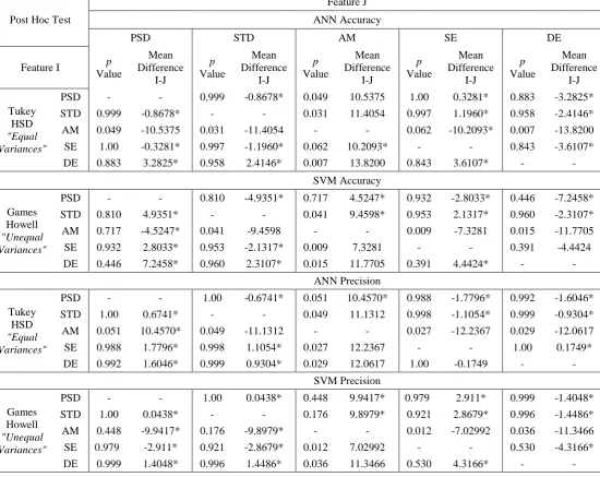
Since significant differences were resulted from features groups in classification performances and differences between features groups was demonstrated by ANOVA test, multiple comparsions were performed with the post-hoc statistical analysis to determine which feature have significant effect in classification algorithm. The data collected from post-hoc statistical test are summarized in Table VI.
Because the ANOVA test was not significant (p>.05) in classification accuracies ,resulted from features groups in Decision tree, LDA and KNN classifiers, multiple comparisons test was not proceed. Therefore there is enough evidence to conclude that different features have no significant interaction effect on accuracy obtained by Decision tree, LDA and KNN classifiers. For ANN classifier post-hoc Tukey HSD's test was carried out to determine which features have significant difference in
classification accuracy. Based on the results of Tukey HSD's test, three significant differences (p-value < .05) for Tukey HSD were found between features-couples Amplitude mean and Differential entropy, between features Amplitude mean and STD, and between Amplitude mean and PSD. The p
value obtained was 0.007, 0.031, and 0.049, respectively (Table VI). Strong evidence (p-value = 0.007) that differential entropy feature have significant effect in classification accuracy more than Amplitude mean feature. Subjects with Differential entropy have on average 13.82% more classification accuracy than those on Amplitude mean. There was also a significant difference between features Amplitude mean and STD (p-value = 0.031). Subjects with Amplitude mean feature have on average 11.40% less classification accuracy than those on STD feature. There is evidance of differences between Amplitude mean and PSD. ANN classifier trained by PSD feature had significantly larger classification accuracy than ANN classifier trained by Amplitude mean feature with average 10.53%. Whereas, no significant differences were found between PSD and STD, between PSD and Differential Entropy, between PSD and Shannon Entropy, between STD and Differential Entropy, between STD and Shannon Entropy, between Differential Entropy and Shannon Entropy, nor between Shannon Entropy and Amplitude mean (p-value > .05) Table VI. Because the classification accuracy in SVM classifier have evidence of non-equality (p-value < .05 Table IV), the post- hoc Tukey HSD test was substituted with Games – Howell's test. Based on the results of Games - Howell's test, no significant differences were found between PSD and STD, between PSD and Amplitude mean, between PSD and Differential Entropy, between PSD and Shannon Entropy, between STD and Differential Entropy, between STD and Shannon Entropy, nor between Differential Entropy and Shannon Entropy (p-value > .05) as shown in Table IV. There are three significant differences (p-value < .05) for Tukey HSD between features Amplitude mean and Differential entropy, between features Amplitude mean and STD, and between Amplitude mean and Shannon entropy. The p values obtained was 0.015, 0.041, and 0.009, respectively (Table VI). Strong evidence (p-value = 0.009) that Shannon entropy feature have significant effect in classification accuracy more than Amplitude mean feature. Subjects with Shannon entropy have on average 7.32% more classification accuracy than those on Amplitude mean. There is also a significant difference between features Amplitude mean and Differential entropy (p-value = 0.015). Subjects with Amplitude mean feature have on average 11.77% less classification accuracy than those on Differential entropy feature. There is evidance of differences between Amplitude mean and STD. ANN classifier which is trained by STD feature had significantly larger classification accuracy than ANN classifier trained by Amplitude mean feature with average 9.45% (Table VI).
(p>.05) in classification precision resulted from features groups in Decision tree, LDA, and KNN classifiers.
For SVM classifier, post-hoc Games - Howell's test was carried out to determine which features have significant difference in classification precision.
No significant differences were found between PSD and STD, between PSD and Amplitude mean, between PSD and Differential Entropy, between PSD and Shannon Entropy, between STD and Differential Entropy, between STD and Amplitude mean, between STD and Shannon Entropy, nor between Differential Entropy and Shannon Entropy (p-value > .05) as shown in Table VI. There are Two significant differences (p-value< .05) for Tukey HSD between features Amplitude mean and Differential entropy, and between Amplitude mean and Shannon entropy. The p value obtained was 0.036, and 0.012, respectively (Table VI). Strong evidence (p-value = 0.012) that Shannon entropy feature have significant effect in classification precision more than Amplitude mean feature. Subjects with Shannon entropy have on average 7.02% more classification precision than those on Amplitude mean. There was also a significant difference between features Amplitude mean and Differential entropy (p-value = 0.036). Subjects with Amplitude mean feature have on average 11.34% less
classification precision than those on Differential entropy feature (Table VI). For classification precision obtained with ANN classifier, differences among features groups were assessed by Tukey HSD's test.
Based on the results of Tukey HSD's test, three significant differences (p-value < .05) for Tukey HSD were found between Amplitude mean and Differential entropy, between features Amplitude mean and STD, and between Amplitude mean and Shannon entropy. The p values obtained was 0.029, 0.049, and 0.027, respectively (Table VI). Evidence (p-value = 0.029) that differential entropy feature have significant effect in classification precision more than Amplitude mean feature. Subjects with Differential entropy have on average 12.06% more classification precision than those on Amplitude mean. There is also a significant difference between Amplitude mean and STD (p-value = 0.049). Subjects with Amplitude mean feature have on average 11.13% less classification precision than those on STD feature. There is evidance of differences between features Amplitude mean and Shannon entropy. ANN classifier trained by Shannon entropy feature had significantly larger classification accuracy than ANN classifier trained by Amplitude mean feature with average 12.23%.Table III shows the values of avrage accuracy values, avrage precision values and avrage MCC values
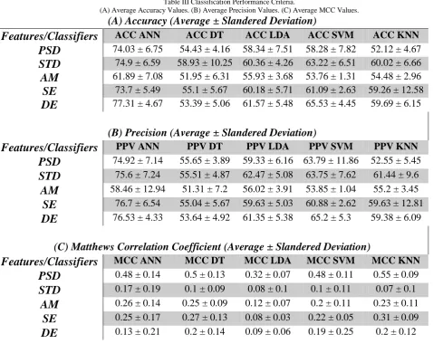
Table III Classification Performance Criteria.
(A) Average Accuracy Values. (B) Average Precision Values. (C) Average MCC Values.
(A) Accuracy (Average ± Slandered Deviation)
Features/Classifiers
ACC ANN
ACC DT
ACC LDA
ACC SVM
ACC KNN
PSD
74.03 ± 6.75
54.43 ± 4.16
58.34 ± 7.51
58.28 ± 7.82
52.12 ± 4.67
STD
74.9 ± 6.59
58.93 ± 10.25
60.36 ± 4.26
63.22 ± 6.51
60.02 ± 6.66
AM
61.89 ± 7.08
51.95 ± 6.31
55.93 ± 3.68
53.76 ± 1.31
54.48 ± 2.96
SE
73.7 ± 5.49
55.1 ± 5.67
60.18 ± 5.71
61.09 ± 2.63
59.26 ± 12.58
DE
77.31 ± 4.67
53.39 ± 5.06
61.57 ± 5.48
65.53 ± 4.45
59.69 ± 6.15
(B) Precision (Average ± Slandered Deviation)
Features/Classifiers
PPV ANN
PPV DT
PPV LDA
PPV SVM
PPV KNN
PSD
74.92 ± 7.14
55.65 ± 3.89
59.33 ± 6.16
63.79 ± 11.86
52.55 ± 5.45
STD
75.6 ± 7.24
55.51 ± 4.87
62.47 ± 5.08
63.75 ± 7.62
61.44 ± 9.6
AM
58.46 ± 12.94
51.31 ± 7.2
56.02 ± 3.91
53.85 ± 1.04
55.2 ± 3.45
SE
76.7 ± 6.54
55.04 ± 5.67
59.63 ± 5.03
60.88 ± 2.62
59.63 ± 12.81
DE
76.53 ± 4.33
53.64 ± 4.92
61.35 ± 5.38
65.2 ± 5.3
59.38 ± 6.09
(C) Matthews Correlation Coefficient (Average ± Slandered Deviation)
Features/Classifiers
MCC ANN
MCC DT
MCC LDA
MCC SVM
MCC KNN
PSD
0.48 ± 0.14
0.5 ± 0.13
0.32 ± 0.07
0.48 ± 0.11
0.55 ± 0.09
STD
0.17 ± 0.19
0.1 ± 0.09
0.08 ± 0.1
0.1 ± 0.11
0.07 ± 0.1
AM
0.26 ± 0.14
0.25 ± 0.09
0.12 ± 0.07
0.2 ± 0.11
0.23 ± 0.11
SE
0.25 ± 0.17
0.27 ± 0.13
0.08 ± 0.03
0.22 ± 0.05
0.31 ± 0.09
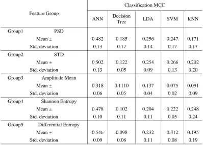
The averaged classification MCC for each training feature with each classification techniques were represented by table VII.Mean classification MCC in ANN classifier were (0.482, 0.502, 0.318, 0.478 and 0.546) for PSD, STD, Amplitude Mean, Shannon entropy and Differential entropy, respectively (table VII). The maximum classification MCC was obtained for Differential entropy feature with mean and standard deviation scores (M=0.546, SD=0.09). The minimum classification MCC in ANN classifier was observed for Amplitude mean feature group with mean and standard deviation scores (M=0.318, SD=0.06). In the second classifier Decision treein table V, mean classification MCC based on (PSD, STD, Amplitude Mean, Shannon entropy and Differential entropy) features groups were (0.185, 0.122, 0.111, 0.102 and 0.098), respectively. The mean and standard deviation scores related to the minimum classification MCC in Decision tree classifier were (M=0.098, SD=0.06) for Differential entropy. Hence, the maximum classification MCC was obtained for PSD feature with mean and standard deviation scores (M=0.185, SD=0.17). for third classification technique "LDA", the maximum classification MCC was observed for PSD feature group with mean and standard deviation scores (M=0.256, SD=0.14) and the minimum classification MCC with mean and standard deviation scores (M=0.137, SD=0.04) were obtained for Amplitude mean feature. Mean classification MCC in LDA classifier were (0.256, 0.254, 0.137, 0.204 and 0.232) for(PSD, STD, Amplitude Mean, Shannon entropy and Differential entropy) features groups, respectively.The mean classification MCC in SVM classifier were (0.247, 0.266, 0.075, 0.222 and 0.312) for PSD, STD, Amplitude Mean, Shannon entropy and Differential entropy, respectively (table V). Minimum classification MCC was observed for Amplitude mean feature group with mean and standard deviation scores (M=0.075, SD=0.02) and the maximum classification MCC with mean and standard deviation scores (M=0.312, SD=0.08) were obtained for Differential entropy feature group. In the final classification technique "KNN", mean classification MCC in were (0.171, 0.202, 0.091, 0.248 and 0.195) for (PSD, STD, Amplitude Mean, Shannon entropy and Differential entropy) features groups, respectively.The mean and standard deviation scores related to the minimum classification MCC were (M=0.091, SD=0.09) for Amplitude mean feature group. Hence, the maximum classification MCC was obtained for Shannon entropy feature with mean and standard deviation scores (M=0.248, SD=0.24).
5–CONCLUSION
In this paper, EEG data for 5 subjects were used as MI-BCI signals. Afterwards, five feathers were extracted from the EEG signals using MATLAB code for each signal and described in the paper theoretically and mathematically. The extracted features were used to train five different classifiers using MATLAB Built-in applications. The next step was to measure the effectiveness of the classification models depending on classification performance metrics which was analyzed statically. Using different classifier techniques on
the EEG signals contained in EEG Motor Imagery Dataset, Significant influence of features groups on the generalization capability of classification system was determined by statistical parametric test one way ANOVA. The classifiers ANN, LDA, Decision tree, SVM and KNN applied on different features groups were used to determine the optimal effects of this trained features on classification performance criteria (Accuracy, Precision and MCC).
The results of classification performance "Accuracy and Precision" vary from feature to feature in two different classifier algorithms. For classification accuracy in ANN classifier, significant differences (p-value < .05) are found between features Amplitude mean and differential entropy, between features Amplitude mean and STD, and between Amplitude mean and PSD. For another pairs features no significant differences was recorded in the other pairs of features. With SVM classifier the ANOVA test demonstrates that the differences in classification accuracies was only significant (p-value < .05) for pairs of features Amplitude mean and Differential entropy, between features Amplitude mean and STD, and between Amplitude mean and Shannon entropy. For LDA, decision tree and KNN classifiers, Different features have no significant interaction effect on accuracy obtained by these classifiers. Also it is important to notice that the significant differences were recorded on classification precisions for some Pairs features " Amplitude mean and Differential entropy, and between Amplitude mean and Shannon entropy" used in classification algorithm SVM. On the otherwise, Significant interaction effect can be obtained in classification precision by Pairs of features "Amplitude mean and Differential entropy, between features Amplitude mean and STD, and between Amplitude mean and Shannon entropy" for ANN classifier. Furthermore, classification precision obtained for classification technique could not be altered with significant difference when using data from different features to train LDA, KNN, and decision tree classifiers. Also, it is possible to get higher average classification MCC in ANN classifier for Differential entropy feature group and the smaller average in SVM classifiers for Amplitude mean feature group. These results have important consideration to determine not only the optimal features but also the significant classifiers. Future work will be focused on a difference between classification techniques for different features in order to record optimal performance criteria and compare it with MCC and other performance criteria "sensitivity and specificity".
6–ACKNOWLEDGMENT
7-FUTURE STUDIES
The theme of this study is simplicity; Simple features were extracted and simple classifiers were applied. Consequently, the next step is to focus on the features and classifiers that give the best performance. More complex studies will be conducted in order to profoundly describe the information contained in EEG signals.
REFERENCES
[1] Philip O. Babalola et.al. (2017). Artificial Neural Network Prediction of Aluminium Metal Matrix Composite with Silicon Carbide Particles Developed Using Stir Casting Method.International Journal of Mechanical & Mechatronics
Engineering IJMME-IJENS Vol:15 No:06.
[2] Nam, C. S., Nijholt, A., & Lotte, F. (Eds.). (2018). Brain– Computer Interfaces Handbook: Technological and Theoretical
Advances. CRC Press.
[3] Wolpaw, J. R., Birbaumer, N., Heetderks, W. J., McFarland, D. J., Peckham, P. H., Schalk, G., ... & Vaughan, T. M. (2000). Brain-computer interface technology: a review of the first international meeting. IEEE transactions on rehabilitation
engineering, 8(2), 164-173.
[4] Mason, S. G., & Birch, G. E. (2003). A general framework for brain-computer interface design. IEEE transactions on neural systems and rehabilitation engineering, 11(1), 70-85.
[5] Solis-Escalante, T. (2012). The Asynchronous Graz Brain
Switch (Doctoral dissertation, Universität Graz).
[6] Lotte, F., Congedo, M., Lécuyer, A., Lamarche, F., &Arnaldi, B. (2007). A review of classification algorithms for EEG-based brain–computer interfaces. Journal of neural engineering, 4(2), R1.
[7] Herman, P., Prasad, G., McGinnity, T. M., & Coyle, D. (2008). Comparative analysis of spectral approaches to feature extraction for EEG-based motor imagery classification. IEEE
Transactions on Neural Systems and Rehabilitation
Engineering, 16(4), 317-326.
[8] Zhao, Q., Zhang, L., &Cichocki, A. (2009). EEG-based asynchronous BCI control of a car in 3D virtual reality environments. Chinese Science Bulletin, 54(1), 78-87.
[9] Shan, H., Xu, H., Zhu, S., & He, B. (2015). A novel channel selection method for optimal classification in different motor imagery BCI paradigms. Biomedical engineering online, 14(1), 93.
[10] Wu, S. L., Liu, Y. T., Hsieh, T. Y., Lin, Y. Y., Chen, C. Y., Chuang, C. H., & Lin, C. T. (2017). Fuzzy integral with particle swarm optimization for a motor-imagery-based brain–computer interface. IEEE Transactions on Fuzzy Systems, 25(1), 21-28. [11] Alansari, M., Kamel, M., Hakim, B., &Kadah, Y. (2018,
January). Study of wavelet-based performance enhancement for motor imagery brain-computer interface. In Brain-Computer
Interface (BCI), 2018 6th International Conference on (pp. 1-4).
IEEE.
[12] Datta, A., & Chatterjee, R. (2019). Comparative Study of Different Ensemble Compositions in EEG Signal Classification Problem. In Emerging Technologies in Data Mining and
Information Security (pp. 145-154). Springer, Singapore.
[13] Alimam, H. et. al. (2017). Design of EMG Acquisition Circuit to Control an Antagonistic Mechanism Actuated by Pneumatic Artificial Muscles PAMs. International Journal of Mechanical
& Mechatronics Engineering IJMME-IJENS Vol:17 No:05.
[14] http://www.bsp.brain.riken.jp/~qibin/homepage/Datasets.html (Accessed: 02/03/2018 20:30).
[15] Welch, P. (1967). The use of fast Fourier transform for the estimation of power spectra: a method based on time averaging over short, modified periodograms. IEEE Transactions on audio
and electroacoustics, 15(2), 70-73.
[16] Harris, F. J. (1978). On the use of windows for harmonic analysis with the discrete Fourier transform. Proceedings of the IEEE, 66(1), 51-83.
[17] Atkinson, J., & Campos, D. (2016). Improving BCI-based emotion recognition by combining EEG feature selection and kernel classifiers. Expert Systems with Applications, 47, 35-41. [18] Tan, D., &Nijholt, A. (2010). Brain-computer interfaces and
human-computer interaction. In Brain-Computer Interfaces (pp. 3-19). Springer London.
[19] Rosso, O. A., Blanco, S., Yordanova, J., Kolev, V., Figliola, A., Schürmann, M., &Başar, E. (2001). Wavelet entropy: a new tool for analysis of short duration brain electrical signals. Journal of
neuroscience methods, 105(1), 65-75.
[20] ao-Guo Xu (2008) Pattern recognition of motor imagery EEG using wavelet transform
[21] Wang, D., Miao, D., &Xie, C. (2011). Best basis-based wavelet packet entropy feature extraction and hierarchical EEG classification for epileptic detection. Expert Systems with
Applications, 38(11), 14314-14320.
[22] Al-Qazzaz, N. K., Hamid Bin Mohd Ali, S., Ahmad, S. A., Islam, M. S., & Escudero, J. (2015). Selection of mother wavelet functions for multi-channel eeg signal analysis during a working memory task. Sensors, 15(11), 29015-29035.
[23] https://www.mathworks.com/help/wavelet/gs/introduction-to-the-wavelet-families.html (Accessed: 04/03/2018 20:30). [24] Yordanova, J., Kolev, V., Rosso, O. A., Schürmann, M.,
Sakowitz, O. W., Özgören, M., &Basar, E. (2002). Wavelet entropy analysis of event-related potentials indicates modality-independent theta dominance. Journal of neuroscience
methods, 117(1), 99-109.
[25] seyyed (2011) Emotion recognition method using entropy analysis of EEG signals
[26] Shi, L. C., Jiao, Y. Y., & Lu, B. L. (2013). Differential entropy feature for EEG-based vigilance estimation. In Engineering in Medicine and Biology Society (EMBC), 2013 35th Annual
International Conference of the IEEE (pp. 6627-6630). IEEE.
[27] Duan, R. N., Zhu, J. Y., & Lu, B. L. (2013, November). Differential entropy feature for EEG-based emotion classification. In Neural Engineering (NER), 2013 6th
International IEEE/EMBS Conference on (pp. 81-84). IEEE.
[28] Konar, A. (1999). Artificial intelligence and soft computing:
behavioral and cognitive modeling of the human brain. CRC
press.
[29] Utgoff, P. E. (1989). Incremental induction of decision trees. Machine learning, 4(2), 161-186.
[30] Akram, F., Han, S. M., & Kim, T. S. (2015). An efficient word typing P300-BCI system using a modified T9 interface and random forest classifier. Computers in biology and medicine, 56, 30-36.
[31] Pfurtscheller G )1999( EEG event-related desynchronization (ERD) and event-related synchronization (ERS)
Electroencephalography: Basic Principles, Clinical
Applications and Related Fields 4th edn, ed E Niedermeyer and
F H Lopes da Silva (Baltimore, MD: Williams and Wilkins) pp 958–67
[32] Krusienski, D. J., Sellers, E. W., Cabestaing, F., Bayoudh, S., McFarland, D. J., Vaughan, T. M., &Wolpaw, J. R. (2006). A comparison of classification techniques for the P300 Speller. Journal of neural engineering, 3(4), 299.
[33] Sammut, C., & Webb, G. I. (Eds.). (2011). Encyclopedia of
machine learning. Springer Science & Business Media.
[34] MehrnazKhodamHazrati. (2013). On Human-Machine Interfaces based on Electrical Brain Signals. Institute for Signal Processing of the University of Lübeck.
[35] Friedman, J., Hastie, T., &Tibshirani, R. (2001). The elements of
statistical learning (Vol. 1, No. 10). New York, NY, USA::
Springer series in statistics.
[36] Haykin, S. S. (2006). New directions in statistical signal
processing: from systems to brain. J. C. Príncipe, T. J.
Sejnowski, & J. McWhirter (Eds.). Cambridge, MA: Mit Press. [37] Boughorbel, S., Jarray, F., & El-Anbari, M. (2017). Optimal
Table VI
A summary of statistical analysis results, Mean of classification accuracies across features groups.
*P>0.05, No significant difference between pair of means to conduct post hoc tests and compare each pair of features groups.
Classification Accuracy
Feature Group
KNN SVM
LDA Decision
Tree ANN
PSD Group1
52.1246 58.2835
58.3401 54.4274
74.0306 Mean ±
0.90 0.23
0.66 0.62
0.24 Shapiro-Wilk
p value
STD Group 2
60.0184 63.2187
60.3572 58.9270
74.8985 Mean ±
0.36 0.48
0.43 0.51
0.95 Shapiro-Wilk
P value
Amplitude Mean Group 3
54.4796 53.7588
55.9303 51.9546
63.4931 Mean ±
0.82 0.20
0.11 0.47
0.11 Shapiro-Wilk
p value
Shannon Entropy Group 4
59.2636 61.0869
60.1833 55.1019
73.7024 Mean ±
0.75 0.65
0.38 0.63
0.73 Shapiro-Wilk
p value
Differential Entropy Group 5
59.6931 65.5294
61.5735 53.3911
77.3131 Mean ±
0.95 0.26
0.33 0.86
0.12 Shapiro-Wilk
p value
ANOVA Assumption
0.734 0.942
0.476 0.439
0.159 Residuals for
Accuracy
p value Levene Test 0.659 0.647 0.215 0.004 0.045
0.346* 0.016
0.538* 0.553*
0.009 One Way
ANOVA
1.189 3.944
0.802 0.777
4.546
Table V
A summary of statistical analysis results, Mean of classification precisions across features groups
*P>0.05, No significant difference between pair of means to conduct post hoc tests and compare each pair of features groups.
Classification Precision
Feature Group
KNN SVM
LDA Decision
Tree ANN
PSD Group1
52.5541 63.7946
59.3272 55.6516
74.9217 Mean ±
0.84 0.76
0.22 0.94
0.59 Shapiro-Wilk
P value
STD Group2
61.4446 63.7508
62.4725 57.5125
75.5959 Mean ±
0.14 0.65
0.97 0.23
0.50 Shapiro-Wilk
P value
Amplitude Mean Group3
55.2003 53.8529
56.0235 51.3051
64.4646 Mean ±
0.12 0.76
0.26 0.50
0.37 Shapiro-Wilk
P value
Shannon Entropy Group4
59.6348 60.8828
59.6274 55.0387
76.7013 Mean ±
0.41 0.98
0.18 0.10
0.99 Shapiro-Wilk
P value
Differential Entropy Group5
59.3776 65.1995
61.3463 53.6358
76.5264 Mean ±
0.99 0.57
0.60 0.92
0.46 Shapiro-Wilk
P value
ANOVA Assumption
0.577 0.277
0.188 0.995
0.702 Residualsfor Precision
P value Levene Test 0.162 0.045 0.756 0.008 0.072
0.434* 0.010
0.372* 0.393*
0.017 One Way ANOVA
0.994 2.207
1.127 1.080
Table VI
A summary of multiple comparisons test results, Feature comparison with Post Hoc test.
* P>0.05, No evidence of difference in classification accuracy between features groups, mean difference (I-J) between pair wise comparison will not be considered.
Feature J
Post Hoc Test ANN Accuracy
Table VII
Averaged classification MCC for different classification techniques applied on the current data set based on different features groups.
Classification MCC
Feature Group
KNN SVM
LDA Decision
Tree ANN
PSD Group1
0.171 0.247
0.256 0.185
0.482 Mean ±
0.17 0.17
0.14 0.17
0.13 Std. deviation
STD Group2
0.202 0.266
0.254 0.122
0.502 Mean ±
0.20 0.13
0.09 0.05
0.13 Std. deviation
Amplitude Mean Group3
0.091 0.075
0.137 0.1110
0.318 Mean ±
0.09 0.02
0.04 0.05
0.06 Std. deviation
Shannon Entropy Group4
0.248 0.222
0.204 0.102
0.478 Mean ±
0.24 0.05
0.11 0.11
0.10 Std. deviation
Differential Entropy Group5
0.195 0.312
0.232 0.098
0.546 Mean ±
0.19 0.08
0.11 0.06
Table VIII List of Abbreviations.
Abbreviation Meaning Notes
MI-BCI Motor Imaginary Brain Computer Interface
-EEG Electroencephalography
-ACC classifier accuracy Performance Metric
LDA Linear discriminant analysis Classifier
RFD Regularized Fischer discriminant Classifier
SVM support vector machine Classifier
PSD Power Spectral Density Signal Feature
ERD event-related desynchronization
-ERS event-related synchronization
-STD Standard Deviation Signal Feature
AM Amplitude Mean Signal Feature
SE Shannon Entropy Signal Feature
DE Differential Entropy Signal Feature
CWT Continues Wavelet Transformation
-ANN Artificial Neural Networks Classifier
K-NN K-nearest Neighbor Classifier
MLP-NN multilayer perceptron neural network Classifier
FLD Fisher’s linear discriminant Classifier
PPV Positive Predicted Value (Classifier Prescient) Performance Metric
TPR True Positive Rate (Classifier Sensitivity) Performance Metric
MCC Matthews Correlation Coefficient Performance Metric
TP True Positive Actual class: Right-hand
Assigned class: Right-hand
FN False Negative Actual class: Right-hand
Assigned class: Left-hand
FP False Positive Actual class: Left-hand
Assigned class: Right-hand
TN True Negative Actual class: Left-hand
Assigned class: Left-hand
Table IX List of Symbols.
Symbol Meaning Units
𝑋(𝑗) Signal Data Volts
PSD
𝑁 Number Of signal’s samples Sample
𝐾 Number; 𝐾 = 1,2,3, … none
𝑊(𝑗) Data Window Volts
𝐿 Segment Length Sample
𝐴𝑘 Finite Fourier Transformation Volts
𝐼𝑘 𝐾 - Modified Periodogram W/Hz
𝑈 Power Data Window Volts2
𝑷̂ Power Spectral Density (PSD) W/Hz
𝒙̅ Amplitude Mean (AM) Volts AM
𝝈 Standard Deviation (STD) Volts STD
𝑊(𝑎, 𝜏) Continues Wavelet Transformation (CWT) Volts
SE
Ψ𝑎,𝜏 Mother Wavelet Volts
𝑎 Scaling Factor none
𝜏 Shifting Factor none
𝐸𝑖 Energy of Each Coefficient Joules
𝐸𝑡𝑜𝑡 Total Energy Joules
𝑃𝑖 Relative Wavelet Energy none
𝐸𝑇 Threshold Entropy none
𝐸𝑙𝑜𝑔 Log Energy Entropy none
𝑬𝑺𝒉 Shannon Entropy (SE) none
𝑋 Random Variable none
DE
𝑓(𝑥) Probability Density Function none

![Table II The structure of Confusion Matrix [29]](https://thumb-us.123doks.com/thumbv2/123dok_us/1351149.1643640/9.595.88.510.78.200/table-ii-structure-confusion-matrix.webp)