Abstract—Recently, several attempts have been made to creating 3D Geographical Information Systems on Web environment from DEM terrain data. However, most of them are facing the Terrain Splitting and Mapping problem which mainly caused by terrains’ sizes and their query capabilities. This problem is a challenge when we want to make ‘truly’ 3D WebGIS systems in equivalent to what have been represented in 2D ones. So far, an algorithm has been presented by Le Hoang Son et al [15] namely as SESA which serves for DEM terrain splitting with minimal memory space in each processor of a computing system. However, this algorithm has some limitations such as computing time and strategies to find solutions. In this paper, we will propose two novel algorithms based on Genetic Algorithm and Particle Swarm Optimization for this problem. The proposed algorithms will be evaluated and compared with SESA algorithm to show their efficiencies.
Index Terms—Genetic Algorithms, Particle Swarm Optimization, SESA, TSM problem.
I. INTRODUCTION
3D Geographical Information System on Web (3D WebGIS) is increasingly important to industrial applications. Some examples of it can be found such as Real Estate Information System [7], [9], [27], Earthquake Disaster Prevention and Mitigation [21], Tourism [8], [19], [24], [28], Traveling [18] and many other ones [1], [20], [25]. In such applications, 3D virtual interfaces modeling terrains or parts of them are provided together with some analysis tools designed for specific problems. The idea behind these 3D WebGIS applications is the capability to manage, control and make decision through a graphical interface with geo-reference supports. As such, more fees or costs can be saved due to ‘better’ decisions are made.
Digital Elevation Model (DEM) [3], [10], [16], [17], [22], [26] is the input of 3D WebGIS systems. DEM terrain data can be in gridded formats, triangulation irregular network (TIN) or contour lines [23]. The most terrain data source used by many GIS applications is gridded DEM. Generally, it is a matrix containing elevation values of all major points in a terrain. These elevation values reflect changes of a terrain in different locations. For example, the mountain area will have equally elevation values on the top of it and higher values than surface area’s ones. An important parameter of DEM terrain is the distances between major points or resolutions. Basically, these numbers are equal and show the accuracy of
Manuscript received March 07, 2011. This work is supported by a research grant of Vietnam National University, Hanoi for promoting Science and Technology.
Le Hoang Son is the corresponding author (e-mail: sonlh@ vnu.edu.vn).
the terrain. Shorter distances increase the number of major points and hence the size of terrain as well. Such large terrains sometimes can not be displayed totally by Web browsers. Indeed, this problem is the first obstacle in deploying 3D WebGIS applications.
Another important limitation of current 3D WebGIS systems is the query capability. Because, DEM terrain contains topographic data only, therefore it is hard to specify which information can be drawn from an area. Without the query capability, we can not perform any analysis functions related to attribute information of the terrain. Indeed, this is the basic problem that should be solved absolutely.
Both limitations above are exactly stated in the Terrain Splitting and Mapping (TSM) problem [15]. This problem is very important in GIS and is the basis for further advance processing tools. Furthermore, it is described as one of some currently promising trends in GIS researches nowadays [11], [12], [13], [14].
In some recent works [15], the authors have proposed two algorithms to solve the TSM problem. Among them, the second one, SESA algorithm, was designed to split a large terrain into some small ones for parallel computing with smallest memory space in each processor of the computing system. However, as we may state in the next section, this algorithm has some limitations and therefore should be ameliorated efficiently.
In this paper, we will present two novel algorithms based on Genetic Algorithm [2] and Particle Swarm Optimization [6] for the TSM problem. Both algorithms are well-suited and tested to be better than SESA algorithm.
The remainder of this paper is organized as follows. Section 2 elaborates the problem. Overview about SESA method will be presented in Section 3. Two novel algorithms are shown in the two next sections. Section 6 presents some results from experiments. Finally, we will make conclusion and future works in the last section.
II. THE PROBLEM
Assume that we have a DEM terrain and some polygons in
2D Polygonal Vector Data (2PVD). Our purpose is to split the original terrain following by these polygons and the number of processors
k
with smallest memory space in all processors. This problem is formulated as followsmin
1
1
=
∑
→
=
k
i i
SP
J
. (1)The constraints are
Heuristic Optimization Algorithms for Terrain Splitting
and Mapping Problem
⎪
⎪
⎩
⎪⎪
⎨
⎧
≠
=
=
×
≤
−
×
≤
j
i
k
j
k
i
S
SP
SP
S
SP
DEM j i DEM i,
,
1
,
,
1
ε
α
, (2)
Where
SP
i ,i
=
1
,
k
are the areas of smallest rectangles containing all polygons in processori
.S
DEM is the area of original terrain. The parameterα
is the saving threshold. The last parameterε
is the difference of areas between two processors. Normally, its range falls into (0, 5).III. RELATED WORKS
As mentioned in previous section, the authors in [15] have proposed the SESA algorithms, the first and only method, to solve the above problem.
The main idea of this algorithm is to traverse all partitions dividing
n
elements intok
blocks. For each partition, calculate its blocks’ areas and check the constraints (2). If finding a suitable partition, stop the algorithm and output the results. Certainly, to reduce the number of traversed partitions, a pre-processing step should be carried out to arrange some elements into specific blocks. Details of this algorithm are summarized as follows.1. Calculate the distance matrix
[ ]
l l ijd
D
×=
where)
,
(
i jij
d
C
C
d
=
is the distance between polygonU
iand
U
j in 2PVD,i
=
1
,
l
,j
=
1
,
l
andi
≠
j
.2. Based on the distance matrix
D
, find an unmarked polygonsU
i and its closet unmarked polygonU
j interm of minimal distance and distance is smaller than
2 2
*
25
.
0
nC
+
nR
until all polygons are reached.3. Calculate the area of polygon
U
i (S
i),U
j (S
j) and bothU
i andU
j (S
ij).4. Additive Condition: If
S
i≥
80
%
S
ij or ijj
S
S
≥
80
%
then we add polygonsU
i andU
jinto a processor.
5. Repeat from Step 2 to Step 4 for other unmarked polygons. The final result is a set of polygons:
{
}
=
≠
≠
>
<
U
i,
U
j,
U
h/
i
,
j
,
h
1
,
k
;
i
j
h
(*)6. Use a parallel partitioning algorithm to divide the set (*) into
k
blocks withk
is the number of processors. In this case, they used the best parallel partitioning algorithm from Hoang Chi Thanh et al. [5].7. For each received block
i
, calculate the area of all polygons in this blockSP
i,i
=
1
,
k
.8. Check the constraints (2). If they are satisfied then stop the partitioning algorithm and perform the Step 6, 7 and 8 of 2OPS algorithm [15] for all current partitions. Otherwise, return to Step 6 to find another solutions.
9. In case of no partitions satisfying the original conditions, conclude that for given parameters
α
andε
, there does not exist any solution for our problem. Therefore, if users want to find other solutions then they should adjust the parameters. For example,%
5
'
=
α
+
α
andε
'
=
ε
+
1
%
. In this situation, return to Step 6 to find other solutions.However, these are two limitations in this algorithm. First, the ‘suitable’ solution found by SESA is not optimal in many cases. In the other words, two parameters
α
andε
are not the smallest ones. Because in the implementation of SESA, the authors [15] constrain the number of iteration steps to ensure the time condition. Therefore, an optimal solution which is not located in these iteration steps can be ignored. Although the main objective of SESA is finding one good solution to reduce the total memory space in all processors, the problem should be increased to specifying the best solution in whole search area. Finally, the last weakness of SESA is its spending time on finding solution. After each number of partitions, the generator re-adjusts the parameters if it can not find any possible solution. This make the answer time is really long in case of no satisfied partition.More details about this method and how to apply it to the TSM problem can be found in [15].
IV. GENETIC ALGORITHM BASED TERRAIN SPLITTING ALGORITHM (GA-TSA)
Genetic algorithm (GA), originally proposed by Dr. John Holland from the University of Michigan in 1975 [2], [4], is a search heuristic that mimics the process of natural evolution. This heuristic is routinely used to generate useful solutions to optimization and search problems. Genetic algorithms belong to the larger class of evolutionary algorithms (EA), which generate solutions to optimization problems using techniques inspired by natural evolution, such as inheritance, mutation, selection, and crossover.
The whole algorithm based on Genetic Algorithm (GA-TSA) is described as follows.
Step 1: Population Initiation
Individual is encoded as a vector
v
=
(
v
1,
v
2,
K
,
v
n)
, withn
is the number of polygons andv
i∈
{
1
,
2
,
K
,
k
}
is the index of part that polygoni
th belong to.( )
1
,
1
,
2
=
v
.
This means polygon
U
1andU
2 are assigned to processor1
P
and polygonU
3 is assigned to processorP
2
.Fig 1. This terrain can be divided into two processors
The beginning population is initiated with
P
individuals (P
is a designed parameter). Each individual is a vector withn
components. Thei
thcomponent is an integer randomly generated within[
1
,
k
]
.Step 2: Calculate fitness values of all individuals in the current population by the following function
{ }
SP
i{
SP
iSP
j}
v
f
−
×
+
×
=
max
max
1
)
(
2
1
γ
γ
, (3)Where
i
=
1
,
k
,
j
=
1
,
k
,
i
≠
j
and(
γ
1,
γ
2)
are ratio constants. The meaning of these couple of parameters is to dynamically adjust the fitness function depending on the most important criteria. Because, it is possible that well fit individual is not always corresponding to a good partition. However, we expect that the satisfied partition is in well fit individuals.Step 3: Select the best-fit individuals for reproduction
Use QuickSort algorithm to sort all individuals following by the ascent of their fitness values. Then, choose the
individuals in the range
⎥⎦
⎤
⎢⎣
⎡
2
,
1
P
to reproduce.Step 4: For each pair of individuals in the list of Step 3, perform Crossover and Mutation operations based on their probabilities to give birth to offspring. Outputted result of this step is a new population
The Crossover operation contains two steps. First, use the Eliticism probability to copy some first individuals from parents to their child. This probability is calculated as
Rate
Eliticism
P
Eliticism
=
*
_
, (4)Where the
Eliticism
_
Rate
is often 0.1.Second, use two randomly best-fit individuals in the previous step to create an offspring from the Eliticism position to the end of the Child. The offsprings are created by single-point probability between their selected parents.
)
,
1
(
Pr
_
obability
Random
n
Single
=
. (5)Fig 4. The Crossover operation Fig 3. First step of Crossover operation
For each created offspring, if its mutation probability is less than a threshold (
GA
_
Mutation
) then we mutate it. The mutative individual is generated by replacing a randomi
v
by another randomv
j,i
=
1
,
n
,j
=
1
,
n
.Fig 5. The Mutation operation
The Crossover and Mutation operations are continued to apply to other offsprings till the end of the Child.
Step 5: Repeat from Step 2 to Step 4 until the number of iteration exceeds a pre-defined maximal iteration step (
GA
_
MaxIter
)Step 6: In case of at least an individual of current population satisfies the constraints (2), find the smallest parameter
α
among all satisfied individuals. Then, perform the Step 6, 7 and 8 of 2OPS algorithm [15] for the optimal individual. Otherwise, no optimal solution is found.This algorithm will guarantee obtaining better results than SESA’s ones. Later, we will check this consideration through Experiment.
V. PARTICLE SWARM OPTIMIZATION BASED TERRAIN SPLITTING ALGORITHM (PSO-TSA)
In this section, we try another method based on Swarm Optimization for our problem.
Particle swarm optimization (PSO) [6] is a population based stochastic optimization technique developed by Dr. Eberhart and Dr. Kennedy in 1995, inspired by social behavior of bird flocking or fish schooling. Generally, it is based on the principle: “The best strategy to find the food is to follow the bird which is nearest to it”. Indeed, in PSO, each single solution is a "bird" or "particle" in the search space. All particles have fitness values which are evaluated by the fitness function to be optimized, and have velocities which direct the flying of the particles. The particles fly through the problem space by following the current optimum particles.
The basic idea of the new algorithm lies on the Seed Procedure. Basically,
k
seeds are evenly distributed in the space. Each seed represents for a number of polygons in 2PVD. Then, we calculate and check the constraints (2). Ifthese criteria are not met, use PSO algorithm to generate a new population until stopping condition is reached.
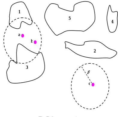
To specify whether a polygon
i
is represented by a seedj
, we use the distance from the center of the smallest rectangle containing polygoni
to this seed. If it is less than a given threshold then we add polygoni
to seedj
.Fig 6. The distance from polygons to a seed point
However, it is possible that some seeds are too close. Therefore, a polygon may be represented by to two or more seeds. Moreover, there exist seeds that do not represent for any polygon. These exceptions are depicted in Fig 7.
1
3
5
2 4 a
b
c
δ
Fig 7. Some exceptions
Therefore, this representation may reduce the number of ‘real’ particles because some of them fall into exceptions. Instead, we perform some adjustments at the positions of seeds. Initially, we choose
k
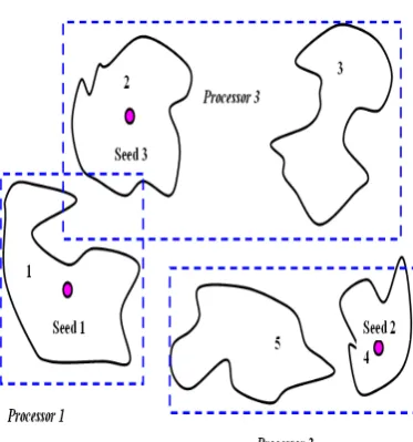
random polygons in 2PVD and mark these centers as seeds. For the rests, they are assigned to the seed that is closet to them.Details about the algorithm based on Particle Swarm Optimization (PSO-TSA) are presented below.
Step 1: Initialization
Each particle is a vector
v
=
(
v
1,
v
2,
K
,
v
k)
wherev
i is the seed pointi
th ,i
=
1
,
k
. These seeds are centers of polygons randomly chosen fromn
polygons of 2PVD. Besides, we also initiate the velocities of these seeds to zeros.For the other polygons, they are assigned to the seed that is closet to them (Fig 9).
Fig 9. Assign remain polygons with n=5 and k=3
Similar process is applied for other particles (Fig 10).
Fig 10. Another particle
Step 2: Calculate fitness values of all particles
In this case, we use the same fitness function (3). Then, the
pBest
value is specified. It is the best value that a particle has reached so far2.1. For each particle
p
[
i
]
2.2. Iff
(
i
)
<
pBest
[
i
]
then 2.3.pBest
[
i
]
=
f
(
i
)
2.4. End If 2.5. End for
. (6)
Step 3: Calculate the global best value gBest among all particles. This is the best value in all iterations
3.1. If
gBest
>
pBest
[
i
]
then 3.2.gBest
=
pBest
[
i
]
3.3. End If
. (7)
Step 4: Calculate new velocities and positions of all seeds similar to the formulae in PSO algorithm [6]
4.1. For each particle
p
[
i
]
4.2. For each velocity j4.3.
]
][
[
*
]
][
[
i
j
c
1velocity
i
j
velocity
=
+
c
2*
rand
()
*
(
seed
[
pBest
][
j
]
−
seed
[
i
][
j
])
+c3*rand()
*
(
seed
[
gBest
][
j
]
−
seed
[
i
][
j
])
4.4. seed[i][j]=seed[i][j]
+
velocity
[
i
][
j
]
4.5. End for 4.6. End for
. (8)
In the formulae above,
c
1 is the ratio to keep the velocity intact,c
2 is the ratio to change the velocity following bypBest
value andc
3 shows the influence level ofgBest
value to the velocity
1
3 2 1
+
c
+
c
=
c
. (9)Step 5: Repeat the whole process from Step 2 to Step 4 until the maximal iteration steps (
PSO
_
MaxIter
) is reached.VI. EXPERIMENTS
In this section, we have implemented the proposed algorithms GA-TSA and PSO-TSA in C programming language and executed them on a PC Core 2 Duo CPU 2 GHz and 1.96 GB of RAM. These algorithms were run against a large DEM terrain whose resolution is 25m and it contains more than 24 million elevation points. The 2PVD is taken from Towns containing 821 polygons (Fig 12). Both data are originated from Bolzano-Bolzen province, Italy in 2005.
Fig 12. Towns Shape
Some parameters initialized in GA-TSA and PSO-TSA are ¾ GA population size:
GA
_
POPSIZE
=
1000
¾ GA maximal iterations:
GA
_
MaxIter
=
100
¾ Eliticism_Rate:
GA
_
ELITRATE
=
0
.
1
¾
GA
_
MUTATIONRA
TE
=
0
.
25
¾
(
γ
1,
γ
2)
=
(
1
,
1
)
¾ PSO population size:
PSO
_
POPSIZE
=
1000
¾ PSO maximal iterations:
PSO
_
MaxIter
=
100
¾
(
c
1,
c
2,
c
3)
=
(
0
.
2
,
0
.
3
,
0
.
5
)
First, we compare the parameter
α
of GA-TSA, PSO-TSA and SESA algorithms when the number of polygons increases and the number of processors is four (Fig 13). Thence, we recognize that with maximalε
=
7
%
, there is not much difference between results of SESA algorithm through different number of polygons. This can be explained as SESA is a greedy algorithm which returns an acceptable, first solution. Indeed, it is possible that a solution can be found in some first iterations of SESA through differentnumber of polygons. Consequently, these results seem unchanged. However, results of SESA algorithm are not optimal and far away from the ones of GA-TSA and PSO-TSA. The parameter
α
found by two proposed algorithms ranges from 2.79% to 20.1% of the parameter found by SESA. Thus, it is obvious that we can save more memory space by using two novel algorithms.Fig 13. Compare the parameter
α
(Alpha) of three algorithmsMoreover, PSO-TSA gives better results than GA-TSA does. Although, these two lines are quite close, however, some differences can be clearly seen when the number of polygons is larger. The average of difference between two algorithms changes from 0.002%, where the number of polygons smaller than 200, to 0.006% where the number of polygons smaller than 500. This difference can be higher if more polygons are added. Therefore, a conclusion can be drawn from this test: PSO-TSA brings smaller parameter
α
than GA-TSA does.Fig 14. Compare the parameter
α
(Alpha) by the number of processorsA similar result can be found at Fig 14 when the number of processors changes. However, the reducing ratio of two algorithms with respect to the SESA algorithm is only from 7.3% to 8.6%. Especially, more processors obtain less memory space in each processor. For example, when the
number of processors is doubled, the average reducing ratio of memory space in each processor is 12% to 25%. Certainly, PSO-TSA still reduces more memory space than GA-TSA does.
Fig 15. The running time of three algorithms
Fig 15 shows the running time of three algorithms following by the number of polygons. The test condition is similar to test 1 in Fig 13. From this, we can easily recognize that SESA is faster than GA-TSA (around 62%) and PSO-TSA (around 21%). The reason we have explained in the previous test. However, this result is quite relative because in some bad cases when the solution lies at the end of iteration steps, the running time of SESA is really long. This consideration was proved in the literature [15].
Fig 16. Compare the running time by the number of processors
The running time of PSO-TSA is 2.3 to 2.9 times slower than GA-TSA. Again, in Fig 16, we re-confirm this consideration. This test compare the running time of three algorithms following by the number of processors. The difference is manifested when the number of processors around 16. At that time, the running time of PSO-TSA is 7 times slower than GA-TSA and 323 times slower than SESA! Obviously, PSO-TSA can bring better parameter
α
, but the cost we have to pay is the running time is too slow. Therefore,a suitable number of processor is required to balance between result and running time. Throughout this test, we think four processors is a suitable answer (Fig 16).
VII. CONCLUSION AND FUTURE WORKS
In this paper, we have investigated two heuristic optimization algorithms for the TSM problem. The first algorithm bases on Evolutionary Optimization, especially Genetic Algorithm (GA-TSA) and the second one PSO-TSA bases on swarm optimization. Both algorithms are implemented and tested through experiments to show the advantages in comparison with the SESA method [15]. Indeed, they are proved to be suitable for the TSM problem and be the basis to deploy further advance computing tools in 3D WebGIS.
In the future, we will look for some other stochastic optimization algorithms for the TSM problem. Moreover, some multi-objectives optimization problems in 3D WebGIS are also our targets.
ACKNOWLEDGMENT
The authors wish to thank anonymous reviewers and the research group at the Center for High Performance Computing, VNU for supporting and giving useful comments. This work is supported by a research grant of Vietnam National University, Hanoi for promoting Science and Technology.
APPENDIX
The source code and test dataset can be found at this address: http://chpc.vnu.vn/gis/heuristic.rar
REFERENCES
[1] CUI YongyiZHOU, DongruWAN, GangFU Huasheng, ”Web VRGIS Study Based on VRML”, Computer Engineering, vol. 8, 2002. [2] Fraser Alex, Donald Burnell, Computer Models in Genetics, New York,
McGraw-Hill, 1970.
[3] GAO Ying-jie et al, “Development of DEM on 1:10000 Scale and Its Application in Geo-sciences”, Journal of Anhui Agricultural Sciences, vol. 2, 2009.
[4] Holland J H, Adaptation in natural and artificial system, Ann Arbor, The University of Michigan Press, 1975.
[5] Hoang Chi Thanh and Nguyen Quang Thanh, “An efficient parallel algorithm for the set partition problem”, New Challenges for Intelligent Information and Database Systems (Ed. Ngoc Thanh Nguyen, Bogdan Trawinski, Jason J. Jung), Springer-Verlag, 2011, accepted.
[6] Kennedy J, Eberhart R, “Particle Swarm Optimization”, In
Proceedings of IEEE International Conference on Neural Networks. IV, 1995, pp. 1942–1948.
[7] LI Lin-lin, CAO Kai-bin, GUAN Bin, ZHU Wei-dong, “Study on the Application of WebGIS and VR in the Information System of Real Estate”, Sci-Tech Information Development & Economy, vol. 5, 2007. [8] LAN Xiaoji, QIU Juxiang, “Digital City GIS-Virtual Tourism”, Land
and Resources Informatization, vol. 1, 2009.
[9] LIN Yao-hua, ZHU Kun-zi, CHEN Jing, “The Development of Putian City Real Estate Information System Based on WEB GIS”, Journal of Xinxiang University (Natural Science Edition), vol. 3, 2009-. [10] LIU Yongqiong, WU Yanlan, HU Hai, HU Peng, “Assessment method
of digital elevation models accuracy and its limitations”, Journal of Geomatics, vol. 5, 2009.
2010 3rd IEEE International Conference on Computer Science and Information Technology (IEEE ICCSIT 2010), Chengdu, China, July 9 - 11, 2010, vol. 1, pp. 182 - 186.
[12] Le Hoang Son, “An Approach to Construct SGIS-3D: a Three Dimensional WebGIS System Based on DEM, GeoVRML and Spatial Analysis operations”, In Proceedings of the 2nd IADIS International Conference Web Virtual Reality and Three-Dimensional Worlds 2010 (IADIS Web3DW 2010), July 27 - 29, 2010, Freiburg, Germany, pp. 317 – 326.
[13] Le Hoang Son, “An Exploratory Study about Spatial Analysis Techniques in Three Dimensional Maps for SGIS-3D systems”, In
Proceedings of the 2010 IEEE International Conference on Electronics and Information Engineering (IEEE ICEIE 2010), August 1 - 3, 2010, Kyoto, Japan, vol. 1, pp. 199 – 203 (ISI Proceeding).
[14] Le Hoang Son, Pham Huy Thong, Nguyen Duy Linh, Truong Chi Cuong and Nguyen Dinh Hoa, “Developing JSG Framework and Applications in COMGIS Project”, International Journal of Computer Information Systems and Industrial Management Applications (IJCISIM), Vol. 3, 2011, pp. 108-118.
[15] Le Hoang Son, Pham Huy Thong, Nguyen Duy Linh, Nguyen Dinh Hoa, and Truong Chi Cuong, “Some Results of 3D Terrain Splitting By 2D Polygonal Vector Data”, International Journal of Machine Learning and Computing (IJMLC), Vol. 1, No. 4, October 2011 (accepted). [16] M. van Kreveld, Digital Elevation Models: overview and selected TIN
algorithms, Algorithmic Foundation of GIS, Springer-Velag, 1997. [17] MA Chi, SONG Wei-dong, “Creating urban DEM by use of
topographic map with DWG format”, Journal of Anshan University of Science and Technology, vol. 5, 2004.
[18] Miao Xuelan, “Application of vrml and webgis technology to the traveling geographic information system”, Computer Applications and Software, vol. 7, 2005.
[19] MA Pengfei, ZHAO Wenji, HU Zhuowei, DUAN Fuzhou, CAI Wenbo , “Research of 3-Dimensional Visualization of Rural Folk Tourism Sight”, Geospatial Information, vol. 5, 2009.
[20] SONG Wei, LI Hua, “Research of 3D Web GIS system based on X3D”,
Computer Engineering and Design, vol. 11, 2005.
[21] SHI Rong, XU Hui-ping, Chen Hua-gen, “Application of 3D Virtual WebGIS in Earthquake Disaster Prevention and Mitigation”, Journal of Seismological Research, vol. 2, 2008.
[22] Sandra Lanig, Arne Schilling, Beate Stollberg and Alexander Zipf, “Towards Standards-Based Processing of Digital Elevation Models for Grid Computing through Web Processing Service (WPS)”, In proceesing of the Computational Science and Its Applications (ICCSA 2008), Lecture Notes in Computer Science, 2008, Volume 5073/2008, pp. 191-203.
[23] S. Rayburga, M. Thomsa and M. Neave, “A comparison of digital elevation models generated from different data sources”,
Geomorphology, Vol. 106, Issues 3-4, 15 May 2009, pp. 261-270. [24] WANG Feng, LIU Ren-yi, LIU Nan, “Study on the application of
WebGIS and virtual reality technology in tourism development”,
Journal of Zhejiang University (Sciences Edition), vol. 6, 2005. [25] WANG Wei,WU Sheng , “Research on the Integration of 3D
Geographic Information Web Services”, Geomatics World, vol. 1, 2008.
[26] WANG Ke-ke, ZHANG Li-chao, PAN Zhen, WANG Qing-shan, ZHANG Shi-quan, “Research on Multiresolution Dynamic Creating Networks Algorithm of DEM based on DirectX”, Beijing Surveying and Mapping, vol. 2, 2008.
[27] YIN Xue-song, “On Real Estate Management Informatization of PKU”,
Research and Exploration in Laboratory, vol. 3, 2009.
[28] ZHANG Yong-fu, LIU Jin-bao, MU Yang, “Analysis and Design of City Tourism Information System Based on WebGIS and Virtual Reality Technology”, Aeronautical Computing Technique, vol. 1, 2008.
Nguyen Duc Thien is a young lecturer at the Faculty of Mathematic, Mechanics and Informatics, Hanoi University of Science, VNU. His research interests include Statistics and Data Mining applications. Email: [email protected]
Le Hoang Son is a researcher at the Center for High Performance Computing, Hanoi University of Science, VNU. He is a member of IACSIT and also member of the editorial board of the International Journal of Engineering and Technology (IJET). His major field includes Data Mining, Geographic Information Systems and Parallel Computing. Email: [email protected]
Pier Luca Lanzi was born in Turin, Italy, in 1967. He received the Ph.D. degree in Computer and Automation Engineering from the Politecnico di Milano in 1999. He is associate professor at the Politecnico di Milano, Dept. of Electronics and Information. His research areas include evolutionary computation, reinforcement learning, machine learning. He is interested in applications to data mining and computer games. He is member of the editorial board of the Evolutionary Computation Journal, the IEEE Transaction on Computational Intelligence and AI in Games, and Evolutionary Intelligence. He is also the founding editor in chief of the SIGEVOlution, the newsletter of the ACM Special Interest Group on Genetic and Evolutionary Computation. He served as the general chair for the 2009 IEEE Conference on Computational Intelligence in Games (CIG-2009) and for the 2011 Genetic and Evolutionary Computation Conference (GECCO-2011). Email: [email protected]