Efficient Graduate Employment Serving System
based on Queuing Theory
Zeng Hui
School of Sciences, Yanshan University, Qinhuangdao, China Email: zenghui @ysu.edu.cn
Abstract—The mathematical model of an two-phases-service M/M/1/N queuing system with the server breakdown and multiple vacations was realized and established in the Graduate Employment Services system. Secondly, equations of steady-state probability were derived by applying the Markov process theory. Then, we obtained matrix form solution of steady-state probability by using blocked matrix method. Finally, some performance measures of the system such as the expected number of users in the system and the queue were also presented.
Index Terms—queuing theory, mathematical model, Graduate Employment Services system
I. INTRODUCTION
Queuing theory is a branch of operations research. The main purpose of the study is to answer how to improve the service provided to an object making a cerain indicator target to achieve optimal [1].Queuing theory originated in 1909 from Copenhagen, Dennark Telephone Company’s A. K Erlang’s famous paper “Probability theory and phone calls” [2]. The thesis of the paper was focused on phone calls creating an applied mathematics in this subject, and many basic principles of the discipline. At present, domestic and international use of queuing theory in the optimization of window and communication facilities. Many researchers have proposed estimation methods of the number of units in circulation and network bandwidth based on queuing theeory.[3, 4]. In recent years, many scholars began to study real-life problems of queuing theory, such as the application in the arrangements in hospital clinics and wards [5, 6], an optimized method for the loading/unloading system of port transportation [7], the application in determining the number of bank teller window and staff [8], the supermarket checkout queue management [9, 10], and a variety of after-sales service system [11]. However, we have not seen any papers about the analysis of Graduate Employment Service system.
The models above only study the case of one service per user provided by each server. In fact, in our daily life, we often encounter a server offering different services for the same users. In such queuing models, all the users need the first phase service and only part of them will be asking the server to provide a second phase service, which is the two-phases-service queuing system. Recently, there have been several contributions
considering queuing system in which the server may provide a second phase service. Madan [12]studied an M/G/1 queue with the second optional service in which first essential service time follows a general distribution but second optional service is assumed to bi exponentially distributed. Medhi [13], generalized the model by considering that the second optional service is also governed by a general distribution. Yue Dequan [14-17], studied an M/M/1/N queue with the multiple vacations; they obtained the matrix form solution of steady-state probability. The system considered in this paper is the secondary server system which is mentioned above.
Graduate Employment Services system is an information service platform that facilitates student’s employment and has a lot of queues in it, and therefore the issue of seeking optimal solution also exists. In this paper we will take a college student employment service system that can accommodate a limited number of users for example, and consider a college student employment service system model in which the server can provide two phases service, and takes a vacation when the system becomes idle. Once service begins, the service mechanism is subject to breakdowns. Parameters are calculated based on actual data and validated to study the performance of its services.
II. SYSTEM MODEL
Graduate Employment Services system capacity is N. Suppose there are only one help desk system for service users. Under normal circumstances, access to the query must be employed to process information, that is, users must first accept the first phase of service. Subsequently, the user will then submit resume online based on their needs, which means choosing to accept the second phase of service. The service mechanism may fail.
A. Input process
In a certain period of time, each user can repeatedly enter the system, so the source of users can be seen as a infinite populaion. Users arrive independently according to Poisson process with different rates. Arrival rate during vacation isλ0, arrival rate during active service is
1
B. Queuing discipline
The first essential service is needed for all arriving users. The vacation times, uninterrupted service times, and the repair times follow exponential distribution. The first service rate isμ1, and the second service rate isμ2.
As soon as the first service of a customer is completed, then with probabilityθ(0< <θ 1), he may opt for the second service, in which case his second service will immediately commence or else with probability1−θ, he may opt to leave the system, in which case another customer at the head of the queue is taken up for his first essential service.
C. Service rules
The server goes on vacation instantly when the queue becomes empty, and continues to take vacations of exponential length until, at the end of a vacation, users are found in the queue. The vacation rate is v and vacation time follows exponential distribution. Service mechanism breakdowns occur only during the first active service, and the breakdown rate isb
(
0< <b 1)
.The service mechanism goes through a repair process of random duration, and once repair is completed, the server returns to the customer whose service was interrupted, the repair rate isr.Various stochastic processes involved in the system are assumed independent of each other.III. STEADY-STATE PROBABILITY EQUATIONS
Let X t( ) be the number of customers in the system at timet. Define C t( ) as the state of the server at the timet. And define the state as follows:
(
)
(
)
(
)
0, The server is on vacation at the time
1, The server is on the first service at the time ( )
2, The server is on the second service at the time
3, The server is on breakdown process at the tim t
t C t
t
=
(
e t)
⎧ ⎪ ⎪ ⎨ ⎪ ⎪ ⎩
Then, { ( ), ( ),X t C t t≥0}is a Makov process with state space as follows:
{( , 0) : 0n n N} {( , ) :1n j n N j, 1, 2, 3}
Ω = ≤ ≤ U ≤ ≤ =
The steady-state probability of the system is defined as follows:
(
)
0( ) lim ( ( ) , ( ) 0), 0 t
p n p X t n C t n N
→∞
= = = ≤ ≤
(
)
( ) lim ( ( ) , ( ) ), 1
j t
p n p X t n C t j n N
→∞
= = = ≤ ≤
By applying the Makov process theory, we can obtain the following set of steady-state probability equations:
0p0(0) 1(1 )p1(1) 2p2(1),
λ =μ −θ +μ (1)
(
)
0 0 0 0
(v+λ )p n( )=λ p n( − ≤ ≤1) , 1 n N−1 (2)
( ) ( 1),
vp N =λ p N− (3)
1 1 1
(
μ λ
+ +b p) (1)0(1) 1(1 ) 1(2) 2 2(2) 3(1),
vp μ θ p μ p rp
= + − + + (4)
1 1 1
(
μ λ
+ +b p n) ( )0( ) 1 1( 1) 1(1 ) 1( 1) vp n λp n μ θ p n
= + − + − +
(
)
2p n2( 1) rp n3( ) , 2 n N
μ
+ + + ≤ ≤ (5)
(
μ1+b p N)
1( )=vp N0( )+λ1p N1( − +1) rp3( )
N , (6)2 1 2 1 1
(μ +λ)p (1)=μ θp(1), (7)
(
)
2 1 2 1 1 1 2
(μ +λ)p n( )=μ θp n( )+λp n( − ≤ ≤1), 2 n N−1 ( 8 )
2p N2( ) 1 p N1( ) 1p N2( 1),
μ =μ θ +λ − (9)
2 3 1
(r+λ )p (1)=bp(1), (10)
(
)
2 3 1 2 3
(r+λ )p n( )=bp n( )+λ p n( − ≤ ≤1), 2 n N−1 (11)
3( ) 1( ) 2 3( 1),
rp N =bp N +λ p N− (12)
0 1 2 3
0 1 1 1
( ) ( ) ( ) ( ) 1.
N N N N
n n n n
p n p n p n p n
= = = =
+ + + =
∑
∑
∑
∑
(13)IV. MATRIX FORM SOLUTION
In the following, we derive the steady-state probability by using the partitioned block matrix method.
Let P=(p0(0),P P P P0, 1, 2, 3) be the steady-state
probability vector of the transition rate matrixQ, where
(
)
0 0(1), 0(2), , 0( )
P = p p L p N
(
(1), (2), , ( ) , 1) (
3)
i i i i
P = p p L p N ≤ ≤i
Then, the steady-state probability equations above can be rewritten in the matrix form as
0 1 PQ Pe
= ⎧ ⎨ =
⎩ (14)
0
0 0
1 1 1
2 2
3 3
0 0 0
0 0 0
0
0 0
0 0 0
A B
Q B C D
B C B D λ η α β ⎛ ⎞ ⎜ ⎟ ⎜ ⎟ ⎜ ⎟ = ⎜ ⎟ ⎜ ⎟ ⎜ ⎟ ⎝ ⎠
Where
e
is a column vector with4
N
+
1
components, and each component of
e
equal to one, and the transition rate matrixQ
of the Markov process has the following blocked matrix structure:0
0 0
1 1 1
2 2
3 3
0 0 0
0 0 0
0
0 0
0 0 0
A B
Q B C D
B C B D λ η α β ⎛ ⎞ ⎜ ⎟ ⎜ ⎟ ⎜ ⎟ = ⎜ ⎟ ⎜ ⎟ ⎜ ⎟ ⎝ ⎠
Each sub-matrix of the matrix
Q
as follows:0 0
0 0
0
0 0
0 0 0
0 0 0
0 0 0
0 0 0 0
v v A v v λ λ λ λ λ λ + − ⎛ ⎞ ⎜ + − ⎟ ⎜ ⎟ ⎜ ⎟ = ⎜ ⎟ + − ⎜ ⎟ ⎜ ⎟ ⎝ ⎠ L L
M M M M M L
L
( )
( )
( )
1 1 1
1 1 1
1
1
1
1 1 1
1 1
0 0
1 0 0
0 1 0 0
0 0 0
0 0
0 0 1
b b B b b μ λ λ μ θ μ λ μ θ λ μ λ λ μ θ μ + + − ⎛ ⎞ ⎜− − + + ⎟ ⎜ ⎟ ⎜ − − ⎟ ⎜ ⎟ = ⎜ ⎟ ⎜ − ⎟ ⎜ ⎟ + + − ⎜ ⎟ ⎜ − − + ⎟ ⎝ ⎠ L L L
M M M M
L L L 2 2 2 2
0 0 0 0
0 0 0
0 0 0
0 0 0
B μ μ μ ⎛ ⎞ ⎜− ⎟ ⎜ ⎟ ⎜ ⎟ = − ⎜ ⎟ ⎜ ⎟ ⎜ − ⎟ ⎝ ⎠ L L L
M M M M L
2 1 1
2 1
2
1
2 1 1
2
0 0
0 0 0
0 0 0
0 0
0 0 0
C μ λ λ μ λ λ μ λ λ μ + − ⎛ ⎞ ⎜ + ⎟ ⎜ ⎟ ⎜ ⎟ = ⎜ ⎟ − ⎜ ⎟ ⎜ + − ⎟ ⎜ ⎟ ⎜ ⎟ ⎝ ⎠ L L
M M M M
L L L 2 2 2 3 2 2 2 0 0
0 0 0
0 0 0
0 0
0 0 0
r r D r r λ λ λ λ λ λ + − ⎛ ⎞ ⎜ + ⎟ ⎜ ⎟ ⎜ ⎟ = ⎜ ⎟ − ⎜ ⎟ ⎜ + − ⎟ ⎜ ⎟ ⎜ ⎟ ⎝ ⎠ L L
M M M M
L L L
(
)
0 1,1, ,1
B = −vdiag K
(
)
3 1,1, ,1
B = −rdiag K
(
)
1 1 1,1, ,1 C = −μ θdiag K
(
)
1 1,1, ,1
D = −bdiag K
Where λ0is a constant,
(
0, 0, , 0)
η= −λ Lis a 1×N row vector,
(
)
(
)
1 1 , 0, , 0 , 2, 0, , 0
T T
α= −⎡⎣ μ −θ L ⎤⎦ β= −μ L
are 1×N column vectors.
(
) (
) (
)
0, i 0 2 , i 1 2 , i 1 3
A B ≤ ≤i C ≤ ≤i D ≤ ≤i are square
matrices.Eq. (14) is rewritten as follows:
( )
0p0 0 P1 P2 0,
λ + α+ β = (15)
( )
0 0 0 0 0, p η+P A =
(16)
0 0 1 1 2 2 3 3 0,
P B +P B +P B +P B = (17)
1 1 2 2 0,
PC +P C = (18)
1 1 3 3 0,
P D +P D = (19)
( )
0 0 0 N 1 N 2 N 3 N 1,
p +P e +Pe +P e +P e = (20)
Where eN is column vector with N components,
and component of eN to one.
From Eq. (2) we get
0 0 0 0 (1) (0) p p v λ λ =
+ (21)
0
0 0
0
( ) (0)
k
p k p
v λ
λ
⎛ ⎞
= ⎜ + ⎟
⎝ ⎠
(
1≤ ≤k N−1)
(22)1 0 0
0 0
0
( ) (0)
N
p N p
v v λ λ λ − ⎛ ⎞ = ⎜ ⎟ +
From Eq. (18), we get
1 2 1 1 2
P = −PC C− (24)
From Eq. (19), we get
1 3 1 1 3
P = −P D D− (25)
Substituting Eq. (24) and (25) into (17), we get
1 1
1 1 1 2 2 1 3 3 0 P B⎡⎣ −C C B− −D D B− ⎤⎦=vP
( )
2 1 1
0 0 0 0
0 0
0 0 0 0
0
, , , ,
N N
v v v
v
v v p
λ λ λ λ λ λ λ λ λ − − ⎛ ⎞ ⎛ ⎞ ⎛ ⎞ ⎜ ⎟ ⎜ ⎟ ⎜ ⎟ + ⎝ + ⎠ ⎝ + ⎠ + ⎛ ⎞ ⎜ ⎟ = ⎜ ⎟
⎝ L ⎝ ⎠ ⎠
(26)
LetA B1 C C B1 21 2 D D B1 31 3
− −
= − − , after some algebraic
manipulation we find the component of the A as follows:
(
)
(
)
(
)
(
)
(
)
(
)
(
)
11 1 1 2
2 1 2
1 2 1 2 1 1 1
2 1 2
1 2 2
2 1 2
2 2 2 2 1 2 2 , ,
1 , 1,
1 , 1
, 1 , 1, , 1, 0, j i ij j i br
b i j N
r
i j N
j i j N
i N j N
br a
i j N
r
br
i j N
r
br
i N j N
r others λ μ λ μ μ θ μ λ λ μ μ μ θ μ λ μ θ μ λ λ λ μ λ λ λ λ λ λ λ − + − + ⎧ + + − + = ≠ ⎪ + + ⎪ ⎪ = = ⎪ ⎪− − − = + ≠ ⎪ + ⎪ − − = = − ⎪ ⎪⎪
= ⎨− −⎪ + < ≤ −
+ + ⎪ ⎪ = = ⎪ + ⎪ ⎪ ⎪− + = − = ⎪ + ⎪ ⎪⎩ , Let 1 2 0 T r A A r ⎛ ⎞ = ⎜ ⎟
⎝% ⎠, each sub-matrix of the matrix A
as follows: ( ) ( ) ( ) ( )( ) ( )( ) ( )( ) ( )( ) ( )( ) ( )( ) ( )( ) ( )( ) ( )( ) ( )
21 22 23 24 25 26 2 1
32 33 34 35 36 3 1
43 44 45 46 4 1
3 4 3 3 3 2 3 1
2 3 2 2 2 1
1 2 1 1
1 0
0 0
0 0 0
0 0 0 0
0 0 0 0 0
0 0 0 0 0 0
N
N
N
N N N N N N N N
N N N N N N
N N N N
N N
a a a a a a a
a a a a a a
a a a a a
A
a a a a
a a a
a a a − − − − − − − − − − − − − − − − − − − − − − ⎛ ⎞ ⎜ ⎟ ⎜ ⎟ ⎜ ⎟ ⎜ ⎟ ⎜ ⎟ ⎜ ⎟ = ⎜ ⎟ ⎜ ⎟ ⎜ ⎟ ⎜ ⎟ ⎜ ⎟ ⎜ ⎟ ⎜ ⎟ ⎝ ⎠ L L L
M M O O O O O M
% L L L L
(
)
1 11, 12, 13, 0, , 0
r = a a a K is a 1×
(
N−1)
row vector,( )
(
)
2 0, , 0, 1 , T T
NN N N
r = K a − a is a 1×
(
N−1)
columnvector. Let
( )
(
)
1 1 1 , 1 P = p P% , Where
( ) ( )
( )
(
)
1 1 2 , 1 3 , , 1
P% = p p K p N .
Eq. (14) is rewritten as follows:
( )
(
( ) ( )
(
)
)
( )
1 1 1 1 0 1 , 0 2 , , 0 1 0 0 p r+P A% %=v p p K p N− =v pσ
(27)
( )
0 1( )
1 2 0 0 0
0
0 N T
P r vp N p
v λ λ λ − ⎛ ⎞ = = ⎜ ⎟ + ⎝ ⎠
% (28)
2 1
0 0 0
0 0 0
, , ,
N
v v v
λ λ λ λ λ λ σ − ⎛ ⎞ ⎛ ⎞ ⎜ ⎟ ⎜ ⎟ + + ⎛ ⎞ ⎜ ⎟ = ⎜ ⎟
⎝ ⎝ ⎠ L ⎝ + ⎠ ⎠
Theorem 1. A% is an invertible matrix, the determinant is
( )1 2
0 N
i i i
A a −
=
=
∏
≠%
Proof. Obviously,
A
%
is an upper triangular matrix, the determinant is equal to the product of diagonalelements, that is ( )1
2 N
i i i
A a −
=
=
∏
% .
For λ λ λ μ μ0, 1, 2, 1, 2, , ,v b r>0 , 0< <b 1,λ λ1, 2≥0 ,
According to the above expression of the aij , that
( )1 0, 2, 3, , i i
a − < i= K N, so A% ≠0. From theorem 1 and Eq. (26), we get
( )
1( )
10 1
we get
( )
1 0 1( )
1 1 2 0 0
0 1 2 1 1 0 N T T
p v A r p
v r A r
λ σ λ λ − − − ⎡ ⎛ ⎞ ⎤ ⎢ ⎥ = − ⎜ ⎟ + ⎢ ⎝ ⎠ ⎥ ⎣ ⎦ % %
( )
0 0 cp= (30) where 1 1 0 2 0 1 0 1 2
1 T N
T
c v A r
v r A r
λ σ λ λ − − − ⎡ ⎛ ⎞ ⎤ ⎢ ⎥ = − ⎜ ⎟ + ⎢ ⎝ ⎠ ⎥ ⎣ ⎦ %
% is a constant.
Substituting Eq. (30) into (29), we get
( )
(
1 1)
1 0 0 1
P% = p v Aσ %− −cr A%− (31)
Let 1 1
1
q=v Aσ %− −cr A%− is a 1×
(
N−1)
row vector, that P%1= p0( )
0 q .So
( )
(
)
( )( )
1 1 1 , 1 0 0 ,
P = p P% = p c q (32) Substituting Eq. (32) into (24),
we get
( )( )
1 2 1 0 0 , 2P =μ θp c q C− (33) Substituting Eq. (32) into (25),
we get
( )( )
13 0 0 , 3
P =bp c q D− (34) Substituting Eq. (16), (33) and (34) into (20),
we get
( )
( )
10 0 0 0 0 N p +p ηA e−
( )( )
( )( )
1 0 0 , N 1 0 0 , 2 N p c q e μ θp c q C e−+ +
( )( )
1 0 0 , 3 N 1 bp c q D e−+ = So
( )
0 0 p =( )
( )
( )
1 1 1
0 1 2 3
1
1+ηA e− N+ c q e, N+μ θ c q C e, − N+b c q D e, − N (35)
Substituting Eq. (35) into (16), (33) and (34), we get the matrix solution ofP P P0, 2, 3. In summary, we have the
following theorem.
Theorem 2. Probability matrix of the steady state solution is:
( )
0 0 p =δ1
0 0
P = −δηA−
( )
1 ,
P =δ c q
( )
12 1 , 2
P =μ θδ c q C−
( )
13 , 3
P =bδ c q D−
Where
1 m
δ =
( )
( )
( )
1 1 1
0 1 2 3
1 N , N , N , N
m= +ηA e− + c q e +μ θ c q C e− +b c q D e−
V. PERFORMANCE MEASURES OF SYSTEM A. The Probability That the System Service Station
During Busy Period
( )
( )
( )
( )
11 2 1 2
1 1 1
, ,
N N N
B
n n n
P p n p n δ c q μ θ c q C−
= = =
⎡ ⎤
=
∑
+∑
=∑
⎣ + ⎦B. The Probability That the System Service Station During Vacation Period
( )
1 10 0 1
0 0
1
N N
V n
n n
P p n δ ηA ε
− − + = = ⎛ ⎞ = = ⎜ − ⎟ ⎝ ⎠
∑
∑
C. The Average Waiting Queue Length of the System
( )
0( )
1(
)
1 1
1
N N
q
n n
E L np n np n
= = =
∑
+∑
+(
)
(
)
2 3 1 1 1 1 N N n nnp n np n
= = +
∑
+ +∑
+( )
( )
( )
1 11 1 2 1
1 1
1 3 1 0 1
, ,
, N
n n
n n n
c q c q C
n N
b c q D A
ε
μ θ
ε
δ
δ
ε
η
ε
− − + + − − = + + ⎡ + ⎤ = ⎢ ⎥+ + − ⎢ ⎥ ⎣ ⎦∑
D. The Average Queue Length of the System
( )
0( )
1( )
1 1
N N
n n
E L np n np n
= = =
∑
+∑
( )
( )
2 3 1 1 N N n nnp n np n
= = +
∑
+∑
1 1 0 1 1 N n nn A N
δ − η −ε δ
+ =
= −
∑
+( )
( )
1( )
11 2 3
1
, , ,
N
n n n
n
n c q c q C b c q D
δ ε μ θ −ε −ε
=
⎡ ⎤
Let εn be a column identity vector of order Nwith is n th component equals to one and the other components equal to zero.
VI. GRADUATE EMPLOYMENT SERVICES SYSTEM
M/M/1/N QUEUING MODEL OF THE CASE STUDY
Based on the above analysis, we obtain the average waiting queue length and the average queue length of the graduate employment services system, and some other state indicators. But as a management decision makers not only to know the steady-state targets, but also to understand some of the parameters on the impact of these state indicators of the system, so that the queuing system as optimal. We take N=5 for example, whenλ0 =λ1=λ2 =1, μ2 =1, b=0.5,v=1, r=1,
1
μ and θ Impact on the average queue length of the system.
Figure 1. The expected waiting queue length E(Lq) vs. the arrival
rateλ1
Figure 2. The expected queue length E(L) vs. the arrival rateλ1
In Figure 1, we fix μ1=μ2 =1 , λ0 =λ2 =1 , 1
v= ,b=1, r=1, θ=0.5. Consider when user’s
increase will find that attendant faster and faster, steady state system in reducing the number of customers. Whenλ1<3, E L
( )
q changes faster. Then, with the λ1increase, the increase of theE L
( )
q gradually slows down.In Figure 2, we fix μ1=μ2=1 , λ0 =λ2 =1 , 1
v= ,b=1, r=1 , θ=0.5. Consider when user’s arrival rateλ1 changes, the average queue length of
changes. Looking at Figure 2, with the λ1 increase will find that attendant faster and faster, steady state system in increasing the number of customers. When λ1<3 ,
( )
E L changes faster. Then, with the λ1 increase, the
increase of the E L
( )
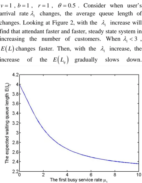
q gradually slows down.Figure 3. The expected waiting queue length E(Lq) vs. the first busy
service rate μ1
Figure 4. The expected queue length E(L) vs. the first busy service rateμ1
In Figure 3, we fixλ0 =λ1=λ2=1,μ2 =1,v=1,b=1, 1
changes. Looking at Figure 3, with the μ1 increase, we will find E L
( )
q first decreases rapidly, steady statesystem in reducing the number of customers. Whenμ1>6, the increase of theE L
( )
q gradually slows down.In Figure 4, we fixλ0=λ1=λ2 =1,μ2=1,v=1,b=1,
1
r= , θ =0.5. Consider when the first busy service rateμ1 changes, the average queue length of changes. Looking at Figure 4, with the μ1 increase, we will find
( )
E L decreases rapidly at first, then in equilibrium.
Figure 5. The expected waiting queue length E(Lq) vs. the
probabilityθof the users chose the second service
In Figure 5, we fixλ0=λ1 =λ2 =1,
1 2 1 μ =μ = ,
1
v= , b=1, r=1, Consider when the probability
θ
of the users chose the second service changes, the expected waiting queue length of changes. Looking at Figure 5, with the number of the user who chose the second service increase, we will find E L( )
q increases linearly withincreasing trend.
Figure 6. The expected queue length E(L) vs. the probabilityθof the users chose the second service
In Figure 6, we fixλ0 =λ1=λ2=1,
1 2 1 μ =μ = ,
1
v= , b=1, r=1, Consider when the probability
θ
of the users chose the second service changes, the average queue length of changes. Looking at Figure 6, with the number of the user who chose the second service increase, we will find E L( )
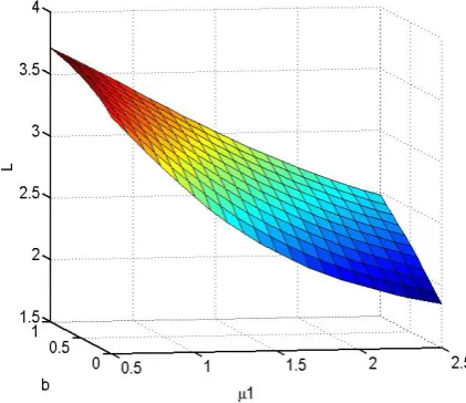
increases linearly with increasing trend.Figure 7. The expected queue length E(L) vs. the service rateμ1and θ
In Figure 7, we fixλ0 =λ1=λ2 =1, μ2 =1,b=0.5 , 1
v= , r=1, and μ1 from 0.5 to 2.5, θfrom 0 to 1.
Looking at Figure 1, with the μ1 increase will find that
attendant faster and faster, steady state system in reducing the number of customers. When μ1 is fixed, with the θ
increases, the average queue length gradually increases.
Figure 8. The expected queue length E(L)vs.the service rateμ1and b
In Figure8, we fixλ0 =λ1=λ2 =1, μ2 =1,θ=0.5, 1
v= , r=1, and μ1 from 0.5 to 2.5, bfrom 0 to 1. Looking at Figure 2, with the μ1 increase will find that
the number of customers. When μ1 is fixed, with the b
increases, the average queue length gradually increases. Through the above analysis, we could get a clearer understanding of the system and some of the parameters on the performance of queuing systems. Using this result, service providers can design a reasonable rate and holiday vacation service rate so that the queuing system could achieve as optimal.
VII. CONCLUSION
Queuing model can be used to the employment services system and its design and to optimize the actual system according to the specific requirements of the system. Queuing system is suitable for analyzing and studying random phenomenon such as the employment service system services. In this paper, the Graduate Employment Services system service queuing model can effectively assess the situation, and support the decision-making with regards to the management and services of the university employment service system.
REFERENCES
[1] Sun Ronghuan, Li Jianping, The Basis of Queuing Theory, Peking: Science, 2002, pp. 1-7.
[2] Zhang Rui, “Analysis of the queuing theory of service industry,” Journal of Qiqihar University Thiliosophy, vol. 6, pp. 41-43, 2002.
[3] Wolff R W, Stochastic Modeling and the Theory of Queues, New York: Prentice Hall, 2000, pp. 23-30.
[4] Meng Yuke, Basic and Applied Queuing Theory, Shang Hai:Tongji University, 1989, pp. 117-120.
[5] Yang Feng, Liu Di, “Queuing theory to improve patient management in the application queue,” University Science Research, vol. 26, pp. 128-129, 2010
[6] Liu Zhan, Xuyange, “The application of queuing theory in the eye’s hospital beds,” China New Technologies and Products, vol. 15, pp. 253-253, 2011.
[7] Huang Daming, Wen Bing, Jiang Shunmei, “An optimized method for the loading/unloading system of port transportation based on queuing theory,” Journal of Guangxi University. Nat Sci Ed, vol. 34, pp. 781-786, 2009.
[8] Sun Zhonghui, “The application of queuing theory in the bank and the teller window,” Operation and Management. vol. 6, pp. 20-21, 2010.
[9] Qin Li, “The application of queuing theory in supermarket checkout service system,” Modern Economy, vol. 10, pp. 7-8, 2009.
[10] Gao Yingying, Zhou Jingzhen, Qian Ting, “The application of queuing theory in library’s service marketing,” SCI-TECH Information Development & Economy, vol. 24, pp. 3-5, 2010.
[11] Kong Xiangping, “The application of queuing theory in the library circulation services system,” The Library Journal of Shangdong, vol. 2, pp. 88-90, 2010.
[12] K.C. Madan, “An M/G/1 queue with second optional service,” Queue. Syst, vol. 34, pp. 37-46, 2000.
[13] J. Medhi, “A single server poisson input queue with a second optional channel,” Queue. Syst., vol. 42, pp. 239-242, 2002.
[14] Yue D, Zhang Y, “Optimal performance analysis of an M/M/1/N queue system with balking, reneging and server vacation,” International Journal of Pure and Applied Mathematics, vol. 28, pp. 101-115, 2006.
[15] Tian R, Yue D, Hu L, “M/ H2 / 1 Queuing System with Balking, N-Policy and Multiple Vacations,” Operation Research and Management Science, vol. 4, pp. 56-60, 2007
[16] Yue D, Sun Y, “The Waiting Time of the M/M/1/N Queuing System with Balking Reneging and Multiple Vacations,” Chinese Journal of Engineering Mathematics, vol. 5, pp. 943 -946, 2008.
[17] Yue D, Sun Y, “The waiting time of M/M/C/N queuing system with balking, reneging and multiple synchronous vacations of partial servers”. Systems Engineering Theory & Practice, vol. 2, pp. 89-97, 2008.