Volume 2008, Article ID 485921,10pages doi:10.1155/2008/485921
Research Article
A Nonlinear Decision-Based Algorithm for
Removal of Strip Lines, Drop Lines, Blotches, Band
Missing and Impulses in Images and Videos
S. Manikandan and D. Ebenezer
Digital Signal Processing Laboratory, Sri Krishna College of Engineering and Technology, Coimbatore, Anna University, Tamilnadu 641008, India
Correspondence should be addressed to S. Manikandan,[email protected]
Received 11 May 2007; Revised 3 December 2007; Accepted 21 July 2008
Recommended by Benoit Macq
A decision-based nonlinear algorithm for removal of strip lines, drop lines, blotches, band missing, and impulses in images is presented. The algorithm performs two simultaneous operations, namely, detection of corrupted pixels and estimation of new pixels for replacing the corrupted pixels. Removal of these artifacts is achieved without damaging edges and details. The algorithm uses an adaptive length window whose maximum size is 5×5 to avoid blurring due to large window sizes. However, the restricted window size renders median operation less effective whenever noise is excessive in which case the proposed algorithm automatically switches to mean filtering. The performance of the algorithm is analyzed in terms of mean square error [MSE], peak-signal-to-noise ratio [PSNR], and image enhancement factor [IEF] and compared with standard algorithms already in use. Improved performance of the proposed algorithm is demonstrated. The advantage of the proposed algorithm is that a single algorithm can replace several independent algorithms required for removal of different artifacts.
Copyright © 2008 S. Manikandan and D. Ebenezer. This is an open access article distributed under the Creative Commons Attribution License, which permits unrestricted use, distribution, and reproduction in any medium, provided the original work is properly cited.
1. INTRODUCTION
It is well known that linear filters are not quite effective in the presence of non-Gaussian noise. In the last decade, it has been shown that nonlinear digital filters can overcome some of the limitations of linear digital filters [1]. Median filters are a class of nonlinear filters and have produced good results where linear filters generally fail [2]. Median filters are known to remove impulse noise and preserve edges. There are a wide variety of median filters in the literature. In remote sensing, artifacts such as strip lines, drop lines, blotches, band missing occur along with impulse noise. Standard median filters reported in the literature do not address these artifacts. Strip lines are caused by unequal responses of elements of a detector array to the same amount of incoming electromagnetic energy [3]. This phenomenon causes heterogeneity in overall brightness of adjacent lines. Drop line [3] occurs when a detector
filtering. Additionally, impulse noise is a standard type of degradation in remotely sensed images. This paper considers application of median-based algorithms for removal of impulses, strip lines, drop lines, band missing, and blotches while preserving edges. It has been shown recently that an adaptive length algorithm provides a better solution for removal of impulse noise with better edge and fine detail preservation. Several adaptive algorithms [6–9] are available for removal of impulse noises. However, none of these algorithms addressed the problem of strip lines, drop lines, blotches, and band missing in images. The objective of this paper is to propose an adaptive length median/mean algorithm that can simultaneously remove impulses, strip lines, drop lines, band missing, and blotches while preserving edges. The advantage of the proposed algorithm is that a single algorithm with improved performance can replace several independent algorithms required for removal of different artifacts.
2. DEGRADED IMAGE MODEL
Blotches are impulsive-type degradations randomly dis-tributed with irregular shapes of approximately constant intensity. These artifacts last for one frame. In the degraded regions there is no correlation between successive frames. Blotches are originated by dust, warping of the substrate or emulsion, mould, dirt, or other unknown causes. Blotches in film sequences can be either bright or dark spots. If the blotch is formed on the positive print of the film, then the result will be a bright spot, however if it is formed on the negative print, then in the positive copy, we will see a dark spot.
Line scratches are narrow vertical, or almost vertical, bright/dark lines that affect a column or a set of columns of the frame. They are also impulsive type artifacts. Line scratches, unlike blotches, can persist for several frames in the same position. The erosion that exists when the film material is run against a foreign object in the jection device causes the line scratches. The transfer pro-cess between film material and telecine can also produce scratches.
It is difficult to propose a general mathematical model for the effect of the abrasion of the film causing the scratches due to the high number of variables that are involved in the process. However, it is possible to make some physical and geometrical considerations regarding the brightness, thickness, and vertical extent of the line. Line scratches can be characterized as follows: (i) they present a considerable higher or lower luminance than their neighborhoods; (ii) they tend to extend over most of the vertical length of the image frame and are not curved; and (iii) they are quite narrow, with widths no larger than 10 pixels for video images. These features can be used to define a model. The degraded image model considered is
a(x,y)=I(x,y)1−b(x,y)+b(x,y)c(x,y), (1)
whereI(x,y) is the pixel intensity of the uncorrupted signal, b(x,y) is a detection variable which is set to 1 whenever
pixels are corrupted and 0 otherwise,c(x,y) is the observed intensity in the corrupted region. This model is applied in this work to images degraded by impulses, strip lines, drop lines, band missing, and blotches.
Ifb(x,y)=0,
thena(x,y)=I(x,y)(1−0) + 0·c(x,y)=I(x,y), (2)
whereI(x,y) is the original pixel value (uncorrupted pixel). Ifb(x,y)=1,
thena(x,y)=I(x,y)(1−1) + 1·c(x,y)=c(x,y), (3)
where c(x,y) is the observed intensity in the corrupted region.
Assume that each pixel at (x,y) is corrupted by an impulse with probability p independent of whether other pixels are corrupted or not. For images corrupted by a neg-ative or positive impulse, the impulse corrupted pixele(x,y) takes on the minimum pixel valuesminwith probabilityp, or
s(x,y) the maximum pixel valuesmaxwith probability 1−p.
The image corrupted by blotches or scratches (impulsive) can be now modeled as
c(x,y)=e(x,y) with p
s(x,y) with 1−p. (4)
This, in fact, is the model that describes impulse noise in the literature. However, the existing impulse filtering algo-rithms do not effectively remove blotches and scratches. In Section 3, an adaptive length median/mean filter algorithm is developed that removes blotches, scratches effectively along with impulse noise.
3. AN ADAPTIVE LENGTH MEDIAN/MEAN FILTER
Median filter is a nonlinear filter, which preserves edges while effectively removing impulse noise. Median operations are performed by row sorting, column sorting, and diagonal sorting in images [10]. General median filters often exhibit blurring for large window sizes, or insufficient noise suppres-sion for small window sizes. Adaptive length median filter overcomes these limitations of general median filters. Lin and Willson [6] proposed an adaptive window length median filter algorithm which can achieve a high degree of noise suppression and still preserve image sharpness; however, the algorithm performs poorly for mixed impulse noise consisting of positive and negative impulses. Lin’s algorithm is modified by Hwang and Haddad [7]. Huang’s algorithm takes into account both positive and negative impulses for simultaneous removal; but it acts poorly on the strip lines, drop lines, and blotches.
blurring. Restriction of window size renders the median operation less effective whenever noise is excessive (the output of the median filter may turn out to be a noisy pixel). In this situation, the algorithm switches to compute the average of uncorrupted pixels in the window (the probability of getting the noisy pixel as filtered output is lower because the averaging takes only uncorrupted pixels into account). The proposed algorithm removes the strip lines, drop lines, blotches along with impulses even at higher noise densities.
4. ILLUSTRATIONS
The algorithm consists of two operations: first is the detection of degraded pixels, and the second operation is the replacement of faulty pixels with the estimated values.
Let the pixel be represented asP(i,j) and the number of corrupted pixels in the windowW(i,j) be “n.” LetPmax =
225 and Pmin = 0 be the corrupted pixel values and
P(i,j)=/0, 255 represent uncorrupted pixels.
Case 1. Consider window size 3 ×3 with typical values of pixels shown as an array below. If P(i,j)=/0, 255, then
the pixels are unaltered. For the array shown, there are no corrupted pixels in the array; therefore, the pixels are unaltered.
123 214 156
236 167 214
123 234 56
(5)
IfP(i,j)=0 or 255, then the following cases are consid-ered (a flow chart illustration of the complete algorithm is shown inFigure 1) .
Case 2. If the number of corrupted pixels “n” in the window W(i,j) is less than or equal to 4, that is,n ≤ 4, then two-dimensional window of size 3×3 is selected and median operation is performed by column sorting, row sorting, and diagonal sorting. The corrupted P(i,j) is replaced by the median value.
0 123 123
0 214 255
234 214 255
0 123 234
0 214 255
123 214 255
123 214 255
0 214 255
0 123 234
255 214 123
0 255 214
123 234 0
Corrupted matrix Row sorting Column sorting Diagonal sorting
(6)
Case 3. If the number of corrupted pixels “n” in the window W(i,j) is between 5 and 12, that is, 5≤n≤12, then perform
5×5 median filtering and replace the corrupted values by the median value.
123 0 156 255 234
255 0 214 98 0
0 234 255 133 190
199 255 234 255 0
255 167 210 198 178
0 123 156 234 255
0 0 98 214 255
0 133 190 234 255
0 199 234 255 255
167 178 198 210 255
0 0 98 210 255
0 123 156 214 255
0 133 190 234 255
0 178 198 234 255
167 199 234 255 255
0 0 98 210 167
0 123 156 178 255
0 133 190 234 255
0 214 198 234 255
255 199 234 255 255
Corrupted matrix Row sorting
Column sorting Diagonal sorting
(7)
Case 4. (i) If the number of corrupted pixels “n” in the windowW(i,j) is greater than 13, that is,n≥13 (a typical
Consider 3×3 window size for image
Calculate the number of corrupted pixels in the window
If
n=0 If
n≤4 If 5< n≤12
Ifn≥13 Yes
Yes
Yes
Yes No
No
No
No Pixels are
unaltered
Perform 3×3 median filtering
Perform 5×5 median filtering
Perform 3×3 median filtering
If all the pixels in 3×3
window is corrupted
Assume 5×5 window size
Replace the processed pixel by average of uncorrupted pixel Repeat the procedure for the next window
(a) Flow chart of the proposed algorithm.
Pixel-wise adaptive window
Input frames
Adaptive median/ mean filtering Temporal median filter
Frame-wise window size=3
Blotch detection
Motion detection
MC filtering
Motion estimation
Output frames
ARPA block matching algorithm pixel-wise (b) Block diagram of the proposed algorithm for video sequences.
median filtering with smaller window sizes, the output may happen to be noise pixels whenever the noise is excessive. In this case, find the average of uncorrupted pixels in the window and replace the corrupted value by the average value.
The average of the pixel value in the window is taken instead of median value, if the number of uncorrupted pixels in the window is even (it is convenient to define median for odd number of pixels).
(133 + 123)/2 = 128
123 0 156 255 234
255 255 123 255 0
0 255 255 133 145
199 0 255 0 255
255 167 0 198 178
255 123 255
255 128 133
0 255 0
255 123 255
255 255 133
0 255 0
(133 and 123 are the uncorrupted pixels)
(8)
(ii) If all the pixels in 3×3 windows are corrupted (a typical case is shown as an array below), then perform 5×5 median filtering. On median filtering, the output may
happen to be noise pixels as in Case4. Find the average of uncorrupted pixels in the window and replace the corrupted value by the average value.
{123+156+234+145+199+167+198+178 = 175
8
175 replaces the corrupted pixel value}
123 0 156 255 234
255 255 0 255 0
0 255 255 255 145
199 0 255 0 255
255 167 0 198 178
255 0 255
255 255 255
0 255 0
123 0 156 255 234
255 255 0 255 0
0 255 175 255 145
199 0 255 0 255
255 167 0 198 178
123 0 156 255 234
255 255 0 255 0
255 255 255 145
199 0 255 0 255
255 167 0 198 178
(9)
5. IMPLEMENTATION IN VIDEO SEQUENCES
The proposed adaptive median/mean algorithm is applied to video sequences degraded by scratches, blotches, and impulses. Adaptive rood pattern search block matching algorithm [11] is used for motion estimation of the image sequences. Motion estimation and compensation techniques [11] are employed for tracking scratches on frames. Predic-tion and interpolaPredic-tion are used to estimate moPredic-tion vectors for video denoising. For fast motion prediction, commonly used technique is block matching (BM) motion estimator. The motion vector is obtained by minimizing a cost function measuring the mismatch between a block and each predictor candidate. The motion estimation (ME) gives motion vector of each pixel or block of pixels which is an essential tool for determining motion trajectories. Due to motion of objects in scene (i.e., corresponding regions in an image sequence), the same region does not occur in the same place in the previous frame as in current one. ARPS [11] algorithm makes use of the fact that the general motion in a frame is usually
coherent, that is, if the macro blocks around the current macro block moved in a particular direction, then there is a high probability that the current macro block will also have a similar motion vector. ARPS algorithm uses the motion vector of the macro block to its immediate left to predict its own motion vector. The rood pattern search directly puts the search in an area where there is a high probability of finding a good matching block. The point that has the least weight becomes the origin for subsequent search steps, and the search pattern is changed to small diamond search pattern (SDSP). SDSP is repeated until least weighted point is found to be at the center of the SDSP. The main advantage of this algorithm over diamond search (DS) is that if the predicted motion vector is (0, 0), it does not waste computational time in carrying out large diamond search pattern (LDSP); it rather directly starts using SDSP.
(a) (b) (c) (d) (e) (f)
Figure2: Drop lines removal. (a) Original image. (b) Corrupted by drop lines. (c) Median filtered image. (d) Lin’s adaptive length filter. (e) Gonzalez adaptive length filter. (f) Proposed algorithm.
(a) (b) (c) (d) (e) (f)
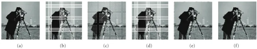
Figure3: Strip lines removal. (a) Original Image. (b) Corrupted by strip lines. (c) Median filtered image. (d) Lin’s adaptive length filter. (e) Gonzalez adaptive length filter. (f) Proposed algorithm.
filtering removes the temporal noise in the form of small dots and streaks found in some videos. In this approach, dirt is viewed as a temporal impulse (single-frame incident) and hence treated by interframe processing by taking into account at least three consecutive frames.Figure 1(b)shows the block diagram of the proposed algorithm implemented in video sequences.
6. RESULTS
The algorithm is tested with different types of degradations, namely, strip lines, drop lines, band missing, blotches, and impulse noise. The results are compared with those of general median filter, Lin’s adaptive length median filter, Gonzalez adaptive length median filter and decision-based median filter.
The median filter and Lin’s algorithm cause blur in the images and do not remove the degradations (Figures 2(c) and 2(d)–Figures 6(c) and 6(d)). The Gonzalez adaptive algorithm removes the strip lines and drop lines but the edges are not preserved properly (Figures2(d)and3(d)) and this algorithm acts very poorly on the blotches and band noises (Figure 4(e)–Figure 6(e)). The proposed algorithm (Figure 2(f)–Figure 6(f)) removes all these degradations more effectively with reduced blurring and edge preserva-tion. The results of the removal of noise at different densities along with degradations are shown in Figures 7 and 8. Lena and Goldhill image are used for comparison.Figure 7 shows 30% of impulse noise with degradations. Figure 8 shows the results of images corrupted with 70% of noise with degradations. Tables 1 and2 show the MSE, PSNR, and IEF values (at different noise densities and artifacts) computed for median filter, Lin’s adaptive length filter,
Gonzalez adaptive length filter, decision-based median filter, and the proposed algorithm. The formulas used are
MSE= 1 mn
m−1
i=0 n−1
j=0
I(i,j)−K(i,j)2,
PSNR=10·log10
MAX2I MSE
=20·log10
MAXI √
MSE
.
(10)
Table1: PSNR, IEF, and MSE for various filters for lena.gif image at different noise densities + degradation. (SMF: standard median filter, AMF: adaptive median filter, DBMF: decision-based median filter, PF: proposed filter).
Noise + degradation PSNR IEF MSE
SMF Lin’s AMF DBMF PF SMF Lin’s AMF DBMF PF SMF Lin’s AMF DBMF PF 0.05 16.5 16.74 17.25 17.95 30.5 3.47 3.6 4.08 4.7 67.05 1430.2 5212 1219.8 1042.2 751.12 0.3 12.94 12.95 16.68 17.73 27.98 2.55 2.5 6.06 7.6 67.64 3244.4 1030 1400.2 1097.5 754.27 0.5 10.20 10.25 14.78 17.35 25.89 1.81 1.83 5.19 9.42 59.38 6103.8 1561 2239.2 1194.6 756.67 0.7 8.07 8.11 11.09 16.60 22.99 1.37 1.39 2.75 9.89 42.60 10030 2181 4940.4 1419.8 807.8
(a) (b) (c) (d) (e) (f)
Figure4: Blotches removal. (a) Original Image. (b) Corrupted by blotches. (c) Median filtered image. (d) Lin’s adaptive length filter. (e) Gonzalez adaptive length filter. (f) Proposed algorithm.
(a) (b) (c) (d) (e) (f)
Figure5: White band noise removal. (a) Original Image. (b) Corrupted by white band noise. (c) Median-filtered image. (d) Lin’s adaptive length filter. (e) Gonzalez adaptive length filter. (f) Proposed algorithm.
(a) (b) (c) (d) (e) (f)
Figure6: Black band noise removal. (a) Original Image. (b) Corrupted by black band noise. (c) Median-filtered image. (d) Lin’s adaptive length filter. (e) Gonzalez adaptive length filter. (f) Proposed algorithm.
(a) (b) (c) (d) (e) (f)
(a) (b) (c) (d) (e) (f)
Figure8: (a) Original images, (b) image corrupted by 70% of impulse noise + degradations, (c) DBMF output, (d) Lin’s adaptive length filter, (e) Gonzalez adaptive length filter, (f) proposed algorithm.
(a) (b) (c) (d)
Figure9: Results: (a) noise (white lines, dark lines) corrupted frames from the black and white film “mannathi mannan,” (b) restored frames by using the proposed algorithm, (c) noise (white lines, dark lines) corrupted frames from the Color film “lesa lesa,” (d) restored color frames by using the proposed algorithm.
(a) (b) (c) (d)
28 28.5 29 29.5 30 30.5 31 31.5 32 32.5
PSNR
0 2 4 6 8 10 12 14 16 18 20
Frame index Spatial median
Temporal median Proposed algorithm
(a)
27 27.5 28 28.5 29 29.5 30 30.5 31 31.5
PSNR
0 2 4 6 8 10 12 14 16 18 20
Frame index Spatial median
Temporal median Proposed algorithm
(b)
Figure11: (a) PSNR comparison graph of “mannathi mannan” black and white film (b) PSNR comparison graph of “lesa lesa” color film.
Table2: PSNR, IEF, and MSE for various filters for goldhill.gif image at different noise densities + degradation.
Noise + degradation PSNR IEF MSE
SMF Lin’s AMF DBMF PF SMF Lin’s AMF DBMF PF SMF Lin’s AMF DBMF PF 0.05 16.21 16.77 17.96 18.78 27.25 3.74 3.57 4.7 5.63 43.79 1308.3 1367 1038.5 859 704.4 0.3 12.82 16.09 17.32 18.48 25.31 2.65 5.3 7.01 9.20 51.61 3232.9 1599 1204.9 921.7 684.6 0.5 10.14 13.48 15.23 18.17 23.84 1.90 3.9 5.84 11.45 46.47 5978.2 2916 1948.7 988.8 657.2 0.7 08.02 09.62 11.20 17.53 22.01 1.41 2.4 2.91 12.47 37.72 10149 7050 4923.2 1148.0 776.1
Table3: PSNR of Lena and Goldhill image corrupted by 20% of impulse noise and the rproposed algorithm corrupted by 20% noise + degradations.
Filter Lena Goldhill
SMF 31.42 29.60
CWMF [12] 30.39 29.87
DBMF [13] 35.12 33.31
Mithra [15] 36.15 34.18
TSMF [14] 31.84 31.53
ACWMF [8] 36.54 34.42
Luo [9]1Anemia 37.05 36.20
PF (noise + degradations) 35.15 35.05
7. CONCLUSION
An adaptive length median/mean algorithm for removal of drops lines, strip lines, white bands, black bands, blotches, and impulses with minimum of blurring is developed. The performance is evaluated in terms of MSE, PSNR, and IEF. The performance is compared with Lin’s adaptive median filter, Gonzalez adaptive median filter, weighted median filter, decision-based median filter and adaptive center
weighted median filter. The results show that the algorithm is more effective in the removal of drop lines, strip lines, white bands, black bands, and blotches along with impulse noise varying upto 70%. The advantage of the proposed algorithm is that a single algorithm with improved performance can replace several independent algorithms required for removal of different artifacts. Application of the proposed algorithm to black and color video sequences is also illustrated.
REFERENCES
[1] J. Astola and P. Kuosmanen,Fundamentals of Nonlinear Digital Filtering, CRC Press, New York, NY, USA, 1977.
[2] I. Pitas and A. N. Venetsanopoulos,Nonlinear Digital Filters: Principles and Applications, Kluwer Academic Publishers, Boston, Mass, USA, 1990.
[3] S. M. Shahrokhy, “Visual and statistical quality assessment and improvement of remotely sensed images,” inProceedings of the 20th Congress of the International Society for Photogrammetry and Remote Sensing (ISPRS ’04), pp. 1–5, Istanbul, Turkey, July 2004.
[5] A. Kokaram, “Detection and removal of line scratches in degraded motion picture sequences,” inProceedings of the 8th European Signal Processing Conference (EUSIPCO ’96), vol. 1, pp. 5–8, Trieste, Italy, September 1996.
[6] H.-M. Lin and A. N. Willson Jr., “Median filters with adaptive length,”IEEE Transactions on Circuits and Systems, vol. 35, no. 6, pp. 675–690, 1988.
[7] H. Hwang and R. A. Haddad, “Adaptive median filters: new algorithms and results,”Transactions on Image Processing, vol. 4, no. 4, pp. 499–502, 1995.
[8] T. Chen and H. R. Wu, “Adaptive impulse detection using center-weighted median filters,”IEEE Signal Processing Letters, vol. 8, no. 1, pp. 1–3, 2001.
[9] W. Luo, “An efficient detail-preserving approach for removing impulse noise in images,”IEEE Signal Processing Letters, vol. 13, no. 7, pp. 413–416, 2006.
[10] K. S. Srinivasan and D. Ebenezer, “A new fast and efficient decision-based algorithm for removal of high-density impulse noises,”IEEE Signal Processing Letters, vol. 14, no. 3, pp. 189– 192, 2007.
[11] Y. Nie and K.-K. Ma, “Adaptive rood pattern search for fast block-matching motion estimation,” IEEE Transactions on Image Processing, vol. 11, no. 12, pp. 1442–1449, 2002. [12] S.-J. Ko and Y. H. Lee, “Center weighted median filters and
their applications to image enhancement,”IEEE Transactions on Circuits and Systems, vol. 38, no. 9, pp. 984–993, 1991. [13] D. A. F. Florencio and R. W. Schafer, “Decision-based median
filter using local signal statistics,” inVisual Communications and Image Processing ’94, vol. 2308 ofProceedings of SPIE, pp. 268–275, Chicago, Ill, USA, September 1994.
[14] T. Chen, K.-K. Ma, and L.-H. Chen, “Tri-state median filter for image denoising,”IEEE Transactions on Image Processing, vol. 8, no. 12, pp. 1834–1838, 1999.