Hourly probabilistic snow forecasts over complex terrain: a hybrid ensemble postprocessing approach

https://doi.org/10.5194/ascmo-4-65-2018 © Author(s) 2018. This work is distributed under the Creative Commons Attribution 4.0 License.

Hourly probabilistic snow forecasts over

complex terrain: a hybrid ensemble

postprocessing approach

Reto Stauffer1, Georg J. Mayr2, Jakob W. Messner3, and Achim Zeileis1

1_{Department of Statistics, Faculty of Economics and Statistics, Universität Innsbruck,}

Universitätsstraße 15, 6020 Innsbruck, Austria

2_{Institute of Atmospheric and Cryospheric Sciences, Faculty of Geo- and Atmospheric Sciences,}

Universität Innsbruck, Innrain 52, 6020 Innsbruck, Austria

3_{Department of Electrical Engineering, Technical University of Denmark, Elektrovej,}

Building 325, 2800 Kgs. Lyngby, Denmark

Correspondence:Reto Stauffer ([email protected])

Received: 27 March 2018 – Revised: 24 August 2018 – Accepted: 12 October 2018 – Published: 14 December 2018

Abstract. Accurate and high-resolution snowfall and fresh snow forecasts are important for a range of economic sectors as well as for the safety of people and infrastructure, especially in mountainous regions. In this article a new hybrid statistical postprocessing method is proposed, which combines standardized anomaly model output statistics (SAMOS) with ensemble copula coupling (ECC) and a novel re-weighting scheme to produce spatially and temporally high-resolution probabilistic snow forecasts. Ensemble forecasts and hindcasts of the European Centre for Medium-Range Weather Forecasts (ECMWF) serve as input for the statistical postprocessing method, while measurements from two different networks provide the required observations.

This new approach is applied to a region with very complex topography in the eastern European Alps. The results demonstrate that the new hybrid method allows one not only to provide reliable high-resolution forecasts, but also to combine different data sources with different temporal resolutions to create hourly probabilistic and physically consistent predictions.

1 Introduction

Large parts of our daily social and economic life strongly rely on weather forecasts. In this article we focus on the gov-ernmental area of Tyrol, Austria, which is located in the east-ern Alps and consists of a large number of narrow valleys surrounded by high mountains. The economic backbone of Tyrol is tourism with more than 5.3 million visitors and more than 25 million overnight stays recorded during the winter season 2013/14 (Amt der Tiroler Landesregierung, 2014). In winter tourism strongly focuses on Alpine outdoor sports such as skiing and back-country skiing, for which resorts and skiing areas need sufficient amounts of snow and good snow conditions. On the other hand, the “white gold” can also cause hazardous situations. During the winter seasons 2009–2016 145 people died in avalanche accidents in

Aus-tria (Lawinenwarndienst Tirol, 2009–2017), of which more than half of all events and deaths occurred in Tyrol. Further-more, severe snow events can obstruct traffic on roads, on train tracks and at airports. Accurate and reliable forecasts of fresh snow and snowfall for the region of Tyrol are therefore of high importance for the public and also for decision mak-ers or warning services (see, e.g., Zhu et al., 2002; Palmer, 2002; Neal et al., 2014; Knox et al., 2015; Raftery, 2016).

sev-eral independent forecasts for the same day using different and slightly perturbed initial conditions and model formu-lations to provide valuable additional information about the uncertainty of a specific weather forecast. Due to the spa-tial discretization of the underlying NWP model the EPS can only depict information on a grid-scale level and is not able to provide reliable information on the point scale. Thus, EPS forecasts typically show too little spread (Hagedorn et al., 2012; Mullen and Buizza, 2001) and require additional cor-rection of the EPS uncertainty to enhance the predictive skill for specific locations. One widely accepted procedure to re-duce possible forecast errors and to adjust the uncertainty information is statistical ensemble postprocessing. Statistical postprocessing methods use historical weather forecasts and the corresponding observations to detect and correct possible systematic EPS errors.

A wide range of different ensemble postprocessing meth-ods have been proposed, including analog methmeth-ods (Hamill et al., 2006, 2015), ensemble dressing methods (Roulston and Smith, 2003), extended logistic regression (Wilks, 2009; Bouallègue and Theis, 2014; Messner et al., 2014b), a non-homogeneous mixture model approach with similarities to Bayesian model averaging (BMA; Sloughter et al., 2007; Fraley et al., 2010), or distributional regression methods. Distributional regression models optimize the parameters of a pre-specified response distribution to correct for both er-rors in the mean and erer-rors in the uncertainty, given a set of covariates. One of the earliest and most well-known ap-proaches is the ensemble model output statistics (EMOS) approach first published by Gneiting et al. (2005) and ap-plied to near-surface temperature. This approach has further been extended by Thorarinsdottir and Gneiting (2010), Lerch and Thorarinsdottir (2013), Scheuerer (2014), Scheuerer and Hamill (2015), Messner et al. (2014a), Scheuerer (2014), Scheuerer and Hamill (2015) and many others for different meteorological quantities using different response distribu-tions and optimization approaches.

Originally, distributional regression was only applied to specific locations, but has also been extended for spatial and even spatio-temporal corrections of the ensemble forecasts. Many of these extensions are based on anomalies (Scheuerer and Büermann, 2014) or standardized anomalies (Dabernig et al., 2017; Stauffer et al., 2017b) to account for location-specific characteristics in mean and variance and create cor-rected and fully probabilistic spatial predictions of temper-ature and daily precipitation sums over potentially complex terrain.

In terms of snow prediction several difficulties have to be considered. The availability and quality of good and reliable snow observations are sparse, even in the region of Tyrol. Measuring snow can be tricky due to possible snow drift, melting processes, or liquid water input (rain) between two observation times, which can yield large measurement errors (Rasmussen et al., 2012). Overall, the amount and quality

of snow measurements make it very difficult to train reliable spatial postprocessing models.

An alternative approach to predict fresh snow amounts is to make use of precipitation and temperature forecasts rather than directly to predict snow. The postprocessed temperature and precipitation forecasts can then be used as a proxy to re-trieve fresh snow amounts and snowfall forecasts. The tem-perature forecasts are on the one hand required to determine whether precipitation reaches the ground as rain or snow and on the other hand to estimate the snow density. Snow density and its alteration are affected by the prevalence of inversions, additional cooling effects due to melting and evaporation of hydrometeors, and other local effects, and are thus an ex-tremely complex issue itself. For simplicity we will only re-gard the problem of whether precipitation occurs as snow or rain and assume that precipitation will fall as snow as soon as the 2 m dry air temperature falls below+1.2◦_{C, a}

thresh-old used in the literature for the European Alps (Rohregger, 2008; Bellaire et al., 2011).

Major challenges of converting probabilistic precipitation and temperature forecasts into fresh snow predictions are the very different temporal resolutions of ensemble predic-tions, temperature observapredic-tions, and precipitation observa-tions. European Centre for Medium-Range Weather Forecast (ECMWF) hindcast and EPS forecasts, which we use in this study, have a temporal resolution of 6 and 1 h, respectively, temperature observations are usually available hourly, and precipitation or snow heights are often only measured once or a few times a day.

In this article we propose a new hybrid approach that combines standardized anomaly model output statistics (SAMOS; Dabernig et al., 2017; Stauffer et al., 2017b) with ensemble copula coupling (ECC; Schefzik et al., 2013) and a novel re-weighting scheme to combine these data to

i. create full probabilistic spatial predictions,

ii. provide probabilistic temperature and precipitation forecasts on an hourly temporal scale, and

iii. create a physically consistent copula (pair of tempera-ture and precipitation) which can be used to

iv. create spatially and temporally high-resolution snowfall and fresh snow amount forecasts.

2 Methods

This section contains the three methodological blocks re-quired to create probabilistic snow forecasts. Distributional regression is explained in Sect. 2.1 followed by the required extensions for the SAMOS in Sect. 2.2. Section 2.3 shows the ensemble copula coupling (ECC) approach to generate a postprocessed ensemble followed by the re-weighting proce-dure in Sect. 2.4 which is required to transform daily precip-itation sums into hourly predictions. Finally, hourly temper-ature and precipitation sums will be converted into probabil-ities of snowfall and fresh snow amounts in Sect. 2.5.

2.1 Distributional regression

Statistical methods considering all parameters of a specific response distribution can be summarized as “distributional regression models”. The EMOS for temperature using a nor-mal response distribution as originally suggested by Gneiting et al. (2005) can be seen as a classical example of this family. Imagine a time series of 2 m temperature observations

y= {yi}i=1, ..., N at a specific site and the corresponding

ensemble forecasts of the 2 m temperature from the EPS x= {xim}m_i=1=1_{, ..., N}, ..., MwhereNdenotes the total sample size of

the data set and M the number of ensemble members. xim

is the individual 2 m temperature prediction of the NWP for date/time i of member m. The EMOS, which slightly dif-fers from the original EMOS as proposed by Gneiting et al. (2005), is specified as

yi ∼N µi, σi, (1)

µi =β0+β1·xi, (2)

log(σi) =γ0+γ1· hxii. (3)

The response yi is assumed to follow a normal

distribu-tion N with the two distributional parametersµi (location

or mean) andσi (scale or standard deviation). Both

param-eters are expressed by a linear predictor including an inter-cept (β0/γ0) and a slope coefficient (β1/γ1) for a covariate.

While the locationµi depends on the ensemble meanxiover

all membersm=1, . . ., Mfor each individual samplei, the log scale depends on the logarithm of the corresponding en-semble standard deviation denoted ashxii. The log link on

σi ensures positive variance in predictions.

The coefficients θ=(β0, β1, γ0, γ1) can be estimated by

using an appropriate M estimator such as the maximum-likelihood estimator maximizing the maximum-likelihood:

ˆ

θ=argmax

θ N

Y

i=1

φ

yi−µi

σi

!

, (4)

where φyi−µi

σi

denotes the standard normal probability density function (PDF) evaluated at each individual i=

1, . . ., Nin the data set.

For the daily precipitation sums the model shown in Eqs. (1)–(3) can be improved by replacing the response dis-tribution and adding an additional covariatezwhich allows one to account for EPS forecasts where the majority of all EPS members predict no precipitation. Following the work of Gebetsberger et al. (2017) and Stauffer et al. (2017a), the model specification can be written as follows:

y_i1/p =L0 µi, σi, (5)

µi =β0+β1·x1i/p·(1−zi)+β2·zi, (6)

log(σi) =γ0+γ1· hx1_i/pi ·(1−zi). (7)

The power-transformed observationsyi are assumed to

fol-low a left-censored logistic distribution L0 censored at 0

and a power parameterp=1.35. The additional covariate zi takes 1 if 80 % or more of all ensemble members predict

less than 0.05 mm over 24 h and 0 otherwise and is used to handle unanimous predictions (cf. Gebetsberger et al., 2017). The correspondingMestimator can be written as

ˆ

θ=argmax

θ N

Y

i=1

f y

1/p

i −µi

σi

!!

with f =   

 

3−µi

σi

if yi =0

λ

y1_i/p−µi

σi

else

, (8)

whereλis the PDF and3the cumulative distribution func-tion (CDF) of the standard logistic distribufunc-tion.

2.2 SAMOS

While the model specifications in Eqs. (1)–(3) and (5)–(7) work well for single stations, an extension is required for spa-tial and/or spatio-temporal ensemble postprocessing. In the following, we will employ the SAMOS approach (Dabernig et al., 2017; Stauffer et al., 2017b) for this purpose. Its basic idea is to remove location- and time-specific characteristics from the observation and EPS data by transforming them into standardized anomalies. This transformation then allows one to fit a single postprocessing model that is valid for the whole area and all season and can thus be applied to any location and time.

Standardized anomalies of the observations (y∗) and EPS forecasts (x∗, for each memberm∈M) will be characterized by a superscript asterisk from here on and are defined as

y_i∗=yi−eµy,i e σy,i

and x_im∗ =xim−eµx,i eσx,i

. (9)

e

in Appendix A. Once the climatologies and thus the stan-dardized anomalies are known, the SAMOS regression coef-ficients can be estimated using Eqs. (1)–(8) by simply replac-ingyi andxi by their corresponding standardized anomalies

y_i∗andx∗_i (except in the condition in Eq. (8) whereyi =0 is

not replaced). Given a new EPS forecast, the postprocessed predictions can be obtained by applying the SAMOS correc-tion. As the regression coefficientsθˆare time and location in-dependent, the correction can be performed on the EPS grid scale. Spatial predictions can be retrieved by bilinearly inter-polating the resulting location (µ∗) and scale (σ∗) parameters to the desired spatial resolution and transforming the results back to the original scale (e.g.,◦C or mm). Algorithm 1 con-tains the pseudo-code for the SAMOS procedure as used for this article.

2.3 Ensemble copula coupling

The SAMOS procedure (Sect. 2.2) provides postprocessed probabilistic predictions for 2 m temperature as well as cor-rected probabilistic forecasts for 24 h precipitation sums. Due to the model specification, SAMOS allows one to re-trieve predictions for any arbitrary location within the area of interest (spatial prediction) and even for all forecast steps covered by the training data set (temporal predictions) with one set of regression coefficients. This allows one to cre-ate forecasts for+30/+54/+78 h for the 24 h precipitation sums, and hourly forecasts for 2 m temperature for the whole study area.

prognos-tic equations, each EPS member provides a distinct physi-cally meaningful combination of temperature and precipita-tion. This property is lost during the SAMOS postprocessing since both quantities are corrected independently. However, the coupling can be restored by drawing a sample of the post-processed predictive distributions and rearranging the sam-pled values in the rank order structure of the original EPS forecasts. ECC is applied to each target location individually to restore the spatial correlation structure of the EPS.

There are different ways to draw a new sample from the postprocessed distributions. It turned out (not shown) that the quantile mapping approach with equidistant probabil-ities (ECC-Q; Schefzik et al., 2013) yields the best and most stable results for this application, which supports the findings of Schefzik et al. (2013). For ECC-Q, a set of M=50+1 ensemble members is drawn from the postpro-cessed distribution based on equidistant probabilities. In the case of the 2 m temperature SAMOS returns hourly esti-mates for location µˆj and scale σˆj of a Gaussian

distribu-tion (Eq. 3; Algorithm 1 step 4iv). Using the inverse Gaus-sian CDF8−1(π| ˆµj,σˆj) with equidistant probabilitiesπ=

1 M+1, . . .,

M

M+1a new 50+1-member temperature ensemble

can be retrieved from the postprocessed distribution. The very same can be done for the daily precipitation sums using the inverse distribution function of the power-transformed left-censored logistic distribution:

3−1₀ π | ˆµj,σˆj, p

=max 0, 3−1(π | ˆµj,σˆj)

p

, (10)

where 3−1 is the inverse CDF of the uncensored logistic distribution. Due to the left-censoring at 0, some of the M quantiles can fall on the censoring point, with an increasing number of 0s with decreasing location µˆj and vice versa.

For situations where precipitation is very unlikelyµˆj might

be highly negative, which yields a postprocessed ensemble where all M members predict exactly 0 mm 24 h−1. How-ever, there is still the problem that our two quantities are not available on the same temporal scale. To be able to restore the full EPS rank order structure on an hourly temporal res-olution the postprocessed daily precipitation sums first have to be downscaled to an hourly interval.

2.4 Precipitation re-weighting

Temperature and precipitation observation data are based on two different observational networks with different temporal resolutions. The 2 m temperature observations are available hourly, while precipitation sums are only reported once a day (details in Sect. 3.3). This temporal resolution is maintained by the SAMOS postprocessing so that it also differs for the forecasts of the different quantities.

As temperature shows a clear diurnal cycle, it is crucial to know at which time of day precipitation is expected to be observed, as the timing can highly affect the precipitation phase and thus the total fresh snow amount. Therefore, the

precipitation forecasts have to be temporally downscaled be-fore they can be combined with the temperature be-forecasts. For this purpose, we extend ECC (Sect. 2.3) with a novel re-weighting scheme where the daily precipitation sums are allocated to the hours of the day according to the time series of the raw EPS predictions. For example, if an EPS member predicts 10 % of its daily precipitation to fall between 10:00 and 11:00, 10 % of the corresponding precipitation forecast is allocated to this hour. This allows one to downscale each of theM=50+1 draws from the marginal precipitation to an hourly temporal resolution and to combine the hourly precip-itation predictions afterwards with the respective draws from the marginal temperature distribution. Algorithm 2 shows the temporal downscaling procedure to generate hourly pre-cipitation copulas from the postprocessed daily prepre-cipitation sums.

For stability reasons, the weights ωare computed using values foryˆj mand tpj mrounded to two digits (₁₀₀1 mm d−1)

to avoid weights close to infinity. Ifyˆj m or tpj m is 0, the

corresponding weight is set to 0 as well. After re-weighting, the precipitation forecasts are at the very same temporal resolution as the temperature forecasts and the rank order structure can be restored with respect to the underlying EPS (Sect. 2.3). This procedure is repeated for each target loca-tion, e.g., on a regular grid with a much finer resolution than the underlying NWP, to create high-resolution spatial predic-tions.

This is necessary as the precipitation postprocessing uses a censored response distribution and a parametric decomposi-tion is not possible (central limit theorem). As a side note it has to be mentioned that the ranks of the hourly copulas are no longer strictly preserved and might sometimes differ from the original rank structure of the EPS.

2.5 New snow amount and probability of snow

Once ECC-Q and re-weighting are applied to the marginal distributions, bi-variate time series of calibrated hourly pre-cipitation sums and 2 m temperatures are available for each of the M ensemble members. For each individual pair of membermand forecast stepsthe “snow indicator function” SImscan be retrieved.

SIms=

           

          

“dry” if

precipitation_ms≤0.05 mm h−1

“rain” if

precipitation_ms>0.05 mm h−1∧T2 m>1.2◦C

“snow” if

precipitation_ms>0.05 mm h−1∧T2 m≤1.2◦C

(11)

The threshold of 0.05 mm h−1 has been chosen as the smallest recorded value of the rain gauges used for valida-tion is 0.1 mm. To distinguish between rain and snow we use a fixed threshold of 1.2◦C as a rough approximation, follow-ing Bellaire et al. (2011, p. 1121). The empirical probabilities πcs for each of the three classes (snow, rain, and dry, which

are mutually exclusive for each individual member and fore-cast time step) or for combinations can be computed using

πcs=

1 M

M

X

m=1

1(SIms=c), (12)

wheresis a specific forecast step andcis the desired class (e.g., snow, rain, rain∨snow).1(·) is an indicator function which takes 1 if the argument in brackets is true or 0 other-wise. The conditional expectation can be derived similarly:

E[c] = PM

i=1precipitationms·1(SIms=c)

PM

i=11(SIms =c)

. (13)

If one is interested in the snow height of fresh snow (E[snow]in centimeters), the snow density has to be taken into account. A rule of thumb is the “1: 10 rule” where 1 mm of liquid water equivalent, the quantity forecasted by the postprocessing, corresponds to 1 cm of fresh snow. This is equivalent to a fresh snow density of 100 kg m−3. In reality, fresh snow densities can vary strongly between 10 and 526 kg m−3given location and prevailing conditions (e.g., Meister, 1985; Judson and Doesken, 2000; Roebber et al., 2003). As reliable fresh snow height or density obser-vations with the desired temporal resolution are not available

for this study, a detailed verification cannot be performed. For visual representation we simply assume a mean density of 100 kg m−3.

3 Data

This section presents the data sets used for this study. These consist of two different EPS forecast data sets (ECMWF hindcast and operational EPS) and three different sources of observation data for model training and verification.

3.1 Numerical weather prediction data: forecast data All predictions presented in this article are based on the ECMWF EPS. The ECMWF EPS consists of 50 perturbed ensemble members and 1 control run (50+1) and is initial-ized four times a day every 6 h. For this study, the control run is treated the same way as the 50 perturbed members. We will solely focus on the 00:00 UTC forecast run of EPS model version43r1. This version became operational on 22 Novem-ber 2016 and the output is available at an hourly temporal resolution up to+90 h ahead on a∼16 km×16 km regular longitude–latitude grid. A visual representation of the grid is shown in Fig. 1.

The presented application will focus on the winter season 2016/17 (1 December 2016 through 15 April 2017) and on predictions from+6 h to+78 h in advance, spanning the first 3 days after EPS initialization (06:00 to 06:00 UTC of 3 con-secutive days).

3.2 Numerical weather prediction data: training data To train the SAMOS models we use ECMWF hindcasts, sim-ilar to the approach of Stauffer et al. (2017b). ECMWF hind-casts become available twice a week (Mondays and Thurs-days), providing a 10+1 member ensemble for the same date over the previous 20 years, initialized at 00:00 UTC. For ex-ample: on Monday 2 January 2017 hindcasts for 2 January 2016, 2015,. . ., 1998, and 1997 become available. As for the EPS, the hindcast control run is treated as an additional mem-ber to increase the ensemble sample size. The hindcasts are available at the same spatial resolution as the EPS, but at a 6-hourly temporal resolution only. To create the training data set for the statistical postprocessing models all hindcasts are bilinearly interpolated to each of the measurement sites (see Sect. 3.3). Overall, 235 different grid points from the numer-ical model are involved in the interpolation for all 199 sites.

3.3 Observational data

Two major different observation networks will be used in the following. As in Stauffer et al. (2017b), daily liquid water equivalent observations from the Tyrol network of hydro-graphical services (EHYD; BMLFUW, 2018) are used for the postprocessing of daily precipitation sums. In compari-son to other networks in the area, the hydrographical service maintains the highest density of stations (number of stations) with very long historical records (up to 47 years of data). The observation sites are well distributed up to an altitude of about 1800 m a.m.s.l. However, observations are only made once a day (manually) at 06:00 UTC. In the following, the observations from 110 sites in and around Tyrol are used to train the precipitation SAMOS models.

The second network consists of 89 automated weather stations operated by the national weather service (TAWES network; Zentralanstalt für Meteorologie und Geodynamik). Seventy-five out of these 89 stations provide at least 6 years of data. Observations are recorded every 10 min, of which all observations at every full hour are used for training and validation of the 2 m air temperature SAMOS models.

The TAWES network also provides automated precipi-tation measurements at a 10 min resolution. However, the length of historical records is much shorter compared to the time series provided by EHYD data set. Furthermore, the measurement errors of the automated rain gauges are ex-pected to be larger than the errors from the daily manual records provided by the hydrographical service, especially during winter. Thus, we decided to not use the TAWES pre-cipitation observations for model training and for the es-timates of the spatio-temporal climatologies. Nevertheless, since observations from the hydrographical service are only available up to 2012 at this time (2018), we do use TAWES precipitation observations for validation. Therefore, daily precipitation sums are generated by taking the sum over all 10 min intervals between 06:10 and 06:00 UTC of the follow-ing day (yields 144 10 min values). Periods for which more than four 10 min values are missing are eliminated.

In addition to the temperature and precipitation observa-tions from the hydrographical service and the TAWES net-work, meteorological aerodrome reports (METARs) from Innsbruck Airport are used in the verification section as it is the only longer-term source of temporally high-resolution

precipitation-phaseobservations available. The weather

con-ditions from the METARs are classified as “snow” (if the report contains SN, SG, IC, PL, SNRA, or RASN), “rain” (if the message contains DZ, RA, SNRA, or RASN), and “dry” (else). Conditions with sleet (mixed rain/snow; SNRA/RASN) are attributed to both “snow” and “rain”. METARs are available every 30 min, created by either a hu-man observer or an automated procedure if the airport is closed over night. These observations have been aggregated to an hourly temporal resolution and will be used to validate the forecasted probabilities of snowfall. Overall, 3318

obser-vations are available for the time period of interest, with 333 cases reporting rain or sleet (10 %), 246 cases snow or sleet (7.5 %), and 2786 cases dry conditions (84 %).

Figure 1 shows an overview of the area of interest. The markers show the locations of the observational sites from the two networks (TAWES, EHYD) and the location of the airport (581 m a.m.s.l.). To the right the height distribution of the stations from the two networks is shown.

4 Statistical models

This section presents the specifications of the models that will be compared and tested in Sect. 5. During the prepara-tion of this paper, a variety of slightly different model formu-lations were tested and the presented models are only a sub-set that was selected because they performed well or showed interesting results.

All the models follow the approaches presented in Sect. 2 but differ in their input variables and whether the data are transformed to standardized anomalies. Four models will be used for 2 m temperature and three for daily precipitation sums. The training data set to estimate the regression co-efficients is composed of all forecast steps provided by the ECMWF hindcasts from +6 up to +78 h on a regular 6 h interval. For precipitation, these forecasts are aggregated to 24 h sums, resulting in forecast steps+30,+54, and+78 h. The power parameter was set top=1.35, found to have the best predictive cross-validated performance in Stauffer et al. (2017b).

Table 1 shows the different model assumptions and nam-ing. The first two models named EMOS correspond to Eqs. (1)–(8) operating on the physical scale (not on standard-ized anomalies). One crucial modification has to be made for the 2 m temperature: interactions with factors for the time of day (hour; 00:00/06:00/12:00/18:00 UTC) and the station

(station) are included to capture spatial and diurnal

differ-ences, yielding separate (and independent) coefficients for each station and each time of day. For daily precipitation sums, this extension has not been made as only 06:00 UTC observations are included (no diurnal effect required) and station-wise regression models partially returned highly un-stable estimates due to the low number of observations for each individual site. Please note that theEMOSmodels are

not designed for spatial or spatio-temporal predictionseven

if spatial predictions would be possible in the case of precip-itation. These two models serve as a reference for the perfor-mance of the SAMOS models.

(a) Station network

10 11 12 13

46.75

47.25

47.75

● ●

●

●

● ●

● ● ●

● ●

● ●

●

● ●

● ●

●

● ●

●

●

● ●

● _● ●●

●

● ●

● ●

● ●

●

● ●

●

● ●

● ● ●

● ●

● ●

●

●

●

●

●

● ●

●

● ●

● ●

● ●

● ●

●●

●

● ●

●

●

● ●

●

● ●

●

●

●

● ●

● ●

●

● ●

● ●

●

● TAWES

EHYD Airport

(b) Height distr.

0 10 20 30

300−600 600−900 900−1200 1200−1500 1500−1800 1800−2100 2100−2400 2400−2700 2700−3000 3000−3300

3300−3600 TAWES

EHYD

Figure 1.Panel(a)shows the topography of the area of interest. Overlays: center of the grid cells of the NWP model data (white crosses), governmental area of Tyrol (black outline), location of the TAWES stations (89; circles) and EHYD stations (110; squares). The airport is indicated by a diamond in the center of the map. Panel(b)shows the height distribution of the stations grouped into 300 m intervals: number of stations (abscissa) and altitude intervals (ordinate; meters a.m.s.l.).

The second and third pairs of models, namedSAMOS_hom

andSAMOS_het, are two SAMOS variations, both solely

us-ing the correspondus-ing quantity from the EPS as a covariate (i.e., 2 m temperature and total precipitation, respectively). While SAMOS_het is a full heteroscedastic model includ-ing the ensemble standard deviation in the linear predictor for the scale σ∗, SAMOS_hom is a homoscedastic model where the scale does not depend on any covariates. These two models allow one to quantify the improvement in the predictive performance by including the ensemble spread in-formation in the postprocessing methods. For 2 m tempera-ture, a fourth model calledxSAMOS_het(x forextended) is used, which includes additional covariates for both location

µ∗_{and scaleσ}∗_{. A set of multilinear models (not shown) has}

been tested that includes different interactions and nonlinear effects in the linear predictors, but no major improvements have been found. Thus, a relatively simple model specifica-tion for xSAMOS_hetis included in this article to demon-strate that SAMOS can easily be extended. The multilinear

xSAMOS_het contains three additional covariates as linear

main effects for both locationµ∗ and scaleσ∗. For each of the covariates separate regression coefficients are estimated during model optimization which, in this case, yields 10 co-efficients in total (one intercept and four covariates in each linear predictor).

5 Results

The first two subsections show the performance of the full predictive distributions of the 2 m temperature (Sect. 5.1) and daily precipitation forecasts (Sect. 5.2). Section 5.3 shows a example of the spatial coherence restored via ECC followed

by a detailed verification of hourly predictions and hourly precipitation-type classification based on the postprocessed ensembles. Last but not least, spatial forecasts for a specific forecast are shown in Sect. 5.6 to demonstrate the feasibility of high-resolution areal predictions.

5.1 Temperature (6 h intervals)

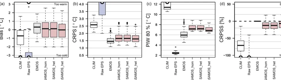
Figure 2 shows bias, continuous rank probability score (CRPS; Gneiting and Raftery, 2007), mean width of the pre-diction interval between the 10 % and 90 % percentiles, and CRPS skill scores, all based on the full predictive distribution returned by the statistical models. All results are temporally out-of-sample and validated on the TAWES network for all forecast steps+6/+12/ . . . /+72/+78 h as used to train the statistical models on hindcasts. The box-and-whiskers show station-wise mean scores for the spatio-temporal climatology (CLIM; Eq. A1), the raw EPS, and the four statistical post-processing models (cf. Table 1).

The raw EPS performs poorly for the area of interest as the NWP model with its current spatial resolution is not able to represent the local topography. It performs even worse than the underlying climatology in terms of bias and CRPS. All statistical postprocessing models perform significantly better and are essentially bias-free. As expected, the station-wise statisticalEMOSmodel performs best since it has separate model coefficients for each station location and is thus more flexible than the spatial models. In terms of CRPS, the spatial models lose about 7 %–12 % of skill (Fig. 2d;SAMOS_hom:

Table 1.Statistical model specification for 2 m temperature (left) and 24 h precipitation sums (right). For each model the linear predictors forµand log(σ) are shown. Superscript asterisk indicate variables on the standardized anomaly scale (SAMOS).T2 m, Td2 m,T850,P, and

tp are the 2 m temperature, 2 m dew point temperature, temperature in 850 hPa, surface pressure, and total precipitation ensemble forecasts respectively.Xare ensemble means,hXidenote ensemble log-standard deviations.X /hour andX /station are interactions betweenXand the “time of the day” and/or the “station”.

Models for 2 m temperature using a Gaussian Models for 24 h precipitation sums using a power-transformed

response distribution. left-censored logistic response distribution.

Heteroscedastic EMOS models (EMOS; cf. Eqs. 1–3 and 5–7)

These modelsare not designed to provide spatial or spatio-temporal predictions.

µ = hour/station+T2 m/hour/station µ = tp1/p·(1−z)+z

log(σ) = hour/station+hT_{2 m}i/hour/station log(σ) =htp1/pi ·(1−z)

Homoscedastic SAMOS models (SAMOS_hom)

µ∗ =T_{2 m}∗ µ∗ = tp1/p∗·(1−z)+z

log(σ∗) = constant log(σ∗) = constant

Heteroscedastic SAMOS models (SAMOS_het)

µ∗ =T_{2 m}∗ µ∗ = tp1/p∗·(1−z)+z

log(σ∗) =hT_{2 m}∗ i log(σ∗) =htp1/p∗i ·(1−z) Extended Heteroscedastic SAMOS models (xSAMOS_het)

µ∗ =T_{2 m}∗ +Td_{2 m}∗ +T₈₅₀∗ +P∗ _–

log(σ∗) =hT_{2 m}∗ i + hTd∗_{2 m}i + hT₈₅₀∗ i + hP∗i –

similarly, indicating that the uncertainty information from the EPS 2 m temperature forecast provides barely any additional information. Small improvements can be achieved by includ-ing additional covariates (modelxSAMOS_het).

Overall, all statistical models show promising values in terms of CRPS (median 1.45–1.65◦C) and mean absolute error (median 2.0–2.3◦C; not shown) across all four meth-ods. The median of the mean prediction interval width for the 10 %–90 % interval is around 6.0◦C for the station-wise

EMOSmodel and around 6.9–7.2◦_{C for the SAMOS models.}

5.2 Daily precipitation sums

Figure 3 shows the verification of the daily precipitation sum predictions for the forecast steps +30/+54/+78 h. Again, this analysis is based on the full predictive distribu-tion returned by the statistical models. Here, the validadistribu-tion is done on different stations (TAWES) than used for model fitting (EHYD; Sect. 3), so that these results are spatially and temporally out of sample. The box-and-whiskers show station-wise mean scores for the spatio-temporal climatol-ogy (CLIM; Eq. A2), the raw daily accumulated total pre-cipitation from the ECMWF EPS (raw EPS), and the three postprocessing methods shown in Table 1.

The top row of Fig. 3 shows bias, CRPS, and the Brier score for probability of precipitation (BS0 mm). The row

be-low shows skill scores with the raw EPS as reference. The two SAMOS models (SAMOS_homandSAMOS_het) show

the best bias among all methods but less predictive skill in terms of MAE, CRPS, and BS0 mm than theEMOS model

not using standardized anomalies. The distinct improvements in the BS0 mm are expected due to the well-known wet bias

of the EPS when comparing interpolated data (spatial scale) to a specific site (point scale). As for 2 m temperature, the use of the forecasted EPS uncertainty in the heteroscedas-tic model (SAMOS_het) brings barely any improvement. The performance of theEMOSmodel requires special attention. Even if this model is not designed to create spatial predic-tions the results show a slightly better performance than the two SAMOS models.

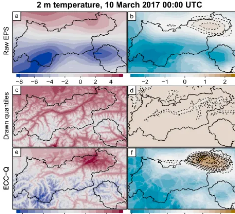
5.3 Spatial coherence (ensemble copula coupling) Sections 5.1 and 5.2 examine the predictive skill of the full probabilistic predictions (SAMOS; Sect. 2.2). The next step is to apply ECC-Q based on the postprocessed hourly 2 m temperature forecasts and daily precipitation sums (Sect. 2.3) to restore the spatial structure of the forecasts.

superimpo-−3 −2 −1 0 1 2 3 ● ● CLIM Ra w E P S EMOS

SAMOS_hom SAMOS_het xSAMOS_het −3 −2 −1 0 1 2 3 ● ● ● Bias [ C] °

(a) Too warm

Too cold 0.5 1.0 1.5 2.0 2.5 3.0 3.5 4.0 ● ● ● ● ● ● ● ● ● ● ● ● ● ● ● ● ● ● ● CLIM Ra w E P S EMOS

SAMOS_hom SAMOS_het xSAMOS_het 0.5 1.0 1.5 2.0 2.5 3.0 3.5 4.0 ● CRPS [ ° C] (b) 2 4 6 8 10 12 ● ● ● ● ● ● ● CLIM Ra w E P S EMOS

SAMOS_hom SAMOS_het xSAMOS_het 2 4 6 8 10 12 ●

PIW 80 % [

° C] (c) −100 −50 0 50 CLIM Ra w E P S EMOS

SAMOS_hom SAMOS_het xSAMOS_het −100 −50 0 50 ● ● CRPSS [%] (d) Better Worse

Figure 2.Scores for 2 m temperature forecasts based on the full predictive distribution based on 6/+12/ . . . /+72/+78 h forecasts as used for model training. The box-and-whisker shows station-wise means for(a)bias (observation minus forecast),(b)CRPS,(c)width of the 80 % prediction interval, and(d)CRPS skill scores withEMOSas reference. Scores are shown for the climatology (CLIM), the raw EPS, and the four postprocessing models (cf. Table 1). Abscissa are set to manually specified ranges; the “semi-sphere” marker (top/bottom) indicates data outside the plotted range.

−4 −3 −2 −1 0 1 2 ● ● ● ● ● ● ● ● ● ● ● ● ● ● ● ● ● ● ● ● ● ● ● ● ● ● ● ● ● ● ● ● −4 −3 −2 −1 0 1 2 (a) Bias [mm] Too wet 0.5 1.0 1.5 2.0 2.5 3.0 3.5 4.0 ● ● ● ● ● ● ● ● ● ● ● ● ● ● ● 0.5 1.0 1.5 2.0 2.5 3.0 3.5 4.0 (b) CRPS [mm] 0.1 0.2 0.3 0.4 0.5 0.6 ● ● ● ● ● ● ● ● ● ● ● ● ● ● ● ● ●●●●● 0.1 0.2 0.3 0.4 0.5 0.6 (c) BS 0mm [mm] −100 −50 0 50 100 ● ● ● ● CLIM Ra w E P S EMOS SAMOS_hom SAMOS_het −100 −50 0 50 100 (d) MAESS [%] Re fe re nc e Better Worse −100 −50 0 50 100 ● ● ● ● CLIM Ra w E P S EMOS SAMOS_hom SAMOS_het −100 −50 0 50 100 (e) CRPSS [%] Re fe re nc e Better Worse 0 20 40 60 80 100 ● ● ● ● ● ● ● ● CLIM Ra w E P S EMOS SAMOS_hom SAMOS_het 0 20 40 60 80 100 (f) BSS 0mm [%] Re fe re nc e Better Worse

Figure 3.Scores for 24 h precipitation sums based on the full predictive distribution for+30,+54, and+78 h forecasts as used for model training. Box-and-whiskers of station-wise mean scores for(a)bias (observation minus forecast),(b)CRPS, and(c)Brier scores for proba-bility of precipitation. The scores are shown for the climatology (CLIM), raw EPS, and the three postprocessing models (cf. Table 1). The lower row shows skill scores for(d)mean absolute error,(e)CRPS, and(f)Brier score for probability of precipitation with theraw EPSas reference. Positive skill scores indicate an improvement over theraw EPS.

sition of location- and elevation-dependent effects. Forecasts and deviations are shown for the raw ensemble, the quantiles drawn from the full probabilistic predictions, and ECC-Q af-ter restoring the rank order structure of the EPS.

As ECC-Q uses quantiles based on equidistant probabil-ities, the quantiles drawn from the full probabilistic distri-bution are ordered. Thus, the forecasts of member 38 (π=

a

Ra

w

E

P

S

−8 −6 −4 −2 0 2 4

c

Dr

aw

n

qu

an

til

es

e

ECC−Q

−15 −10 −5 0 5

b

−2 −1 0 1 2

d

f

ECC−Q

−6 −4 −2 0 2 4 6

2 m temperature, 10 March 2017 00:00 UTC

Figure 4.2 m temperature forecasts of member 38 for 10 March 2017 00:00 UTC. Top–down: raw EPS (a, b), unsorted quan-tile(c, d), and ECC-Q(e, f)after restoring the rank order structure. Forecast (a, c, e;◦C) and deviation of this forecast from the median of the corresponding ensemble (b, d, f;◦C) are shown. Overlays: contours for positive deviation (dashed) and the borders of the gov-ernmental area of Tyrol (solid). Please note that the color scale of the top row differs from the scale of the two lower rows.

(π=0.5) before the rank order structure is restored. This can be seen in Figs. 4d and 5d, where the deviation against the en-semble median is plotted. In this case the deviation is (more or less) a constant positive offset across the whole domain with only little spatial structure. These small spatial features are induced by the SAMOS procedure where the data are transformed into the standardized anomaly scale and back to the physical scale (Sect. 2.2) and are not associated with the spatial coherence of the EPS (cf. Figs. 4b and 5b). To restore the spatial structure, the quantiles have to be reordered given the rank order structure of the raw EPS at each of the target locations. The bottom rows of Figs. 4 and 5 show the fore-casts after rearranging the quantiles. In contrast to the non-rearranged forecasts (middle row) the postprocessed fore-casts with restored rank-order structure exhibit a very similar spatial coherence to the raw EPS (top row of Figs. 4 and 5). The coherence of the EPS is maintained unchanged in large parts, but is not identical as it is slightly modified by the post-processing procedure.

5.4 Hourly temperature and precipitation sums

Sections 5.1 and 5.2 show that the postprocessing models are able to improve the predictive performance of the raw EPS for temperature and daily precipitation sums. The main goal of this study is to provide accurate and reliable snow

a

Ra

w

E

P

S

5 10 15 20 25 30 35 40 45

c

Dr

aw

n

qu

an

til

es

e

ECC−Q

0 20 40 60 80 100

b

−15 −10 −5 0 5 10 15

d

f

ECC−Q

−40 −20 0 20 40

Daily precipitation sum, 10 March 2017 06:00 UTC

Figure 5.As Fig. 4 but for daily precipitation sums valid 9 March 2017 06:00 UTC to 10 March 2017 06:00 UTC. Forecasts(a, c, e)

and deviations from the ensemble median(b, d, f)are shown in mm 24 h−1. In contrast to Fig. 4 contours are plotted for negative deviations.

predictions by combining hourly 2 m temperature and pre-cipitation forecasts. Thus, an hourly temporal resolution for both temperature and precipitation forecasts is required. This section therefore shows the verification of hourly forecasts. For temperature, the hourly forecasts are based on the spatio-temporal SAMOS modelxSAMOS_hetas it shows the over-all best performance among over-all tested spatial models. The hourly precipitation sums are based on the predictions from

the SAMOS_het model downscaled to the desired

tempo-ral resolution using the re-weighting approach presented in Sect. 2.4. Since the re-weighted precipitation forecasts are only available as ensembles but not as full predictive distri-butions, ensemble verification methods are employed in the following.

Hourly 2 m temperature, raw EPS

0.00

0.01

0.02

0.03

0.04

0.05

1 7 13 19 25 31 37 43 49

Rank

Density

(a)

Hourly 2 m temperature, ECC−Q

0.00

0.01

0.02

0.03

0.04

0.05

1 7 13 19 25 31 37 43 49

Rank

Density

(b)

Hourly precipitation sums, raw EPS

0.00

0.01

0.02

0.03

0.04

0.05

1 7 13 19 25 31 37 43 49

Rank

Density

(c)

Hourly precipitation sums, ECC−Q

0.00

0.01

0.02

0.03

0.04

0.05

1 7 13 19 25 31 37 43 49

Rank

Density

(d)

Multivariate rank histogram, raw EPS

0.00

0.01

0.02

0.03

0.04

0.05

1 7 13 19 25 31 37 43 49

Rank

Density

(e)

Multivariate rank histogram, ECC−Q

0.00

0.01

0.02

0.03

0.04

0.05

1 7 13 19 25 31 37 43 49

Rank

Density

(f)

Figure 6.(Stacked) ensemble rank histograms for hourly 2 m tem-perature (a, b)and hourly precipitation sum forecasts(c, d)plus multivariate rank histogram(e, f)of the raw EPS(a, c, e)and post-processed copula(b, d, f)with 50+1 members each. The rank his-tograms contain all available forecasts for all stations and forecast steps +7,+8, . . .,+78 h in advance. For precipitation, the faded colors show the rank histogram for all forecasts where 50 % or more of all members predicted 0 mm h−1. Please note that theyaxis is cut at 0.05 for all histograms.

rank shows the rank histogram of the full verification data set. The faded colors show the calibration for all forecasts where at least 50 % of all members forecasted 0 mm h−1(dry cases). It can be seen that the dry cases are relatively well calibrated and that the majority of the underdispersion results from the wet cases. Nevertheless, the asymmetry (decreasing density with increasing rank) indicates a small wet bias also for the dry cases.

To score the multivariate skill of the combined temperature and precipitation forecasts, the bottom row of Fig. 6 shows multivariate (bivariate) rank histograms (Gneiting et al., 2008). In contrast to the univariate rank histograms the multi-variate rank histogram takes the rank order structure between the two quantities into account. As for the univariate rank his-tograms the multivariate rank histogram shows much better calibration of the postprocessed predictions but shows very similar patterns to the two univariate histograms (Fig. 6a–c).

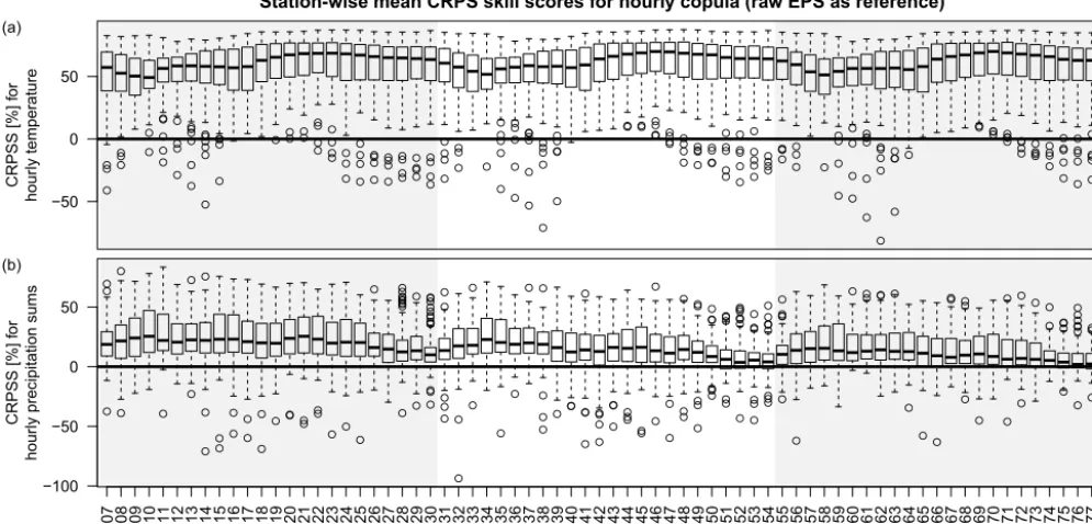
To investigate the univariate predictive performance of hourly predictions for different forecast horizons, Fig. 7 shows CRPS skill scores for all individual lead times. Each box-and-whisker contains station-wise mean skill scores over the verification period. While always on a high level, the 2 m temperature forecasts for morning hours (+7 to 12,+31 to 36,+55 to 60, corresponding to 07:00–12:00 UTC) show slightly less skill. For precipitation, the skill scores are over-all positive but clearly decreasing with increasing forecast horizon. The lowest skill scores are found for early morning hours (+26 to 30,+50 to 54,+74 to 78; 02:00–06:00 UTC).

5.5 Fresh snow amounts and probability of snowfall This section shows the verification for the main target vari-able. Due to the limited availability of temporally high-resolution and reliable observations this can only be done for one site, the regional airport in Innsbruck (Fig. 1). Fig-ure 8 shows reliability diagrams (Bröcker and Smith, 2007) for the probability of precipitation (rain∨snow), rain, and snow. As Sect. 5.4 indicates that large parts of the improve-ments are expected to come from temperature postprocess-ing, three different models will be compared: the raw EPS, the full ECC-Q, and a mixed version. The mixed version uses the raw hourly precipitation forecasts from the EPS but the postprocessed temperature predictions to examine the con-tribution of the precipitation postprocessing. The validation for all three methods is based on the classification described in Sect. 2.5 and the aggregated METAR observations as de-scribed in Sect. 3.3.

For all three precipitation classes ECC-Q is able to outper-form the raw EPS (less off-diagonal) and shows lower Brier scores and lower numbers for reliability while losing some resolution. ECC-Q is also beneficial over the mixed ver-sion using uncorrected precipitation sums. For snow the two methods using postprocessed temperature forecasts (mixed and ECC-Q) perform very similarly but show different bi-ases. While the mixed model exhibits a wet bias (observed frequencies larger than forecasted probabilities), ECC-Q shows a dry bias. The results for snow should not be over-interpreted as snowfall is relatively rare at this station (7.5 % of all cases). The raw EPS again shows the well-known wet bias in all three classes.

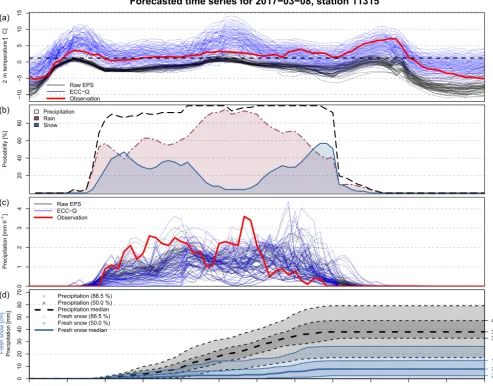
Next, Fig. 9 shows a forecast time series example for a ran-dom station and a day when the temperature is just around 1.2◦C, the threshold used to decide whether the forecasted precipitation will fall as snow or rain. As no fresh snow mea-surements are available, a validation of the forecasted fresh snow amounts cannot be performed for this case.

● ● ● ● ● ● ● ● ● ● ● ● ● ● ● ● ● ● ● ● ● ● ● ● ● ● ● ● ● ● ● ● ● ● ●●●● ● ● ● ● ● ● ● ● ● ● ● ● ● ● ● ● ● ● ● ● ● ● ● ● ● ● ● ● ● ● ● ● ● ● ● ● ● ● ● ● ● ● ● ● ● ● ● ● ● ● ● ● ● ● ● ● ● ● ● ● ● ● ● ● ● ● ● ● ● ● ● ●● ● ● ● ● ● ● ● ● ● ● ● ● ● ● ● ● ● ● ● ● ● ● ● ● ● ● ● ● ● ● ● ● ● ● ● ● ● ● ● ● ● ● ● ● ● ● ● ● ● ● ● ● ● ● ● ● ● ● ● ● ● ● ● ● ● ● ● ● ● ● ● ● ● ●●● ● ● ● ● ● ● ● ● ● ● ● ● ●●● ● ● ● ● ● ● ● ● ● ● ● ● ● ● ● ● ● ● ● ● −50 0 50

CRPSS [%] f

or

hour

ly temper

ature

Station-wise mean CRPS skill scores for hourly copula (raw EPS as reference)

(a) ● ● ● ● ● ● ● ● ● ● ● ● ● ● ● ● ● ● ● ●●●●_●●● ●●_● ● ● ● ● ● ● ● ● ● ● ● ● ● ● ● ● ● ● ● ● ● ● ● ● ● ● ● ● ● ● ● ● ● ● ● ● ● ● ● ● ● ● ●●● ● ● ● ● ● ● ● ● ● ● ● ● ● ● ● ● ● ● ● ● ● ● ● ● ● ● ● ● ● ● ● ● ● ● ● ● ● ● ● ● ● ● ● ● ● ● ● ● ● ● ● ● ● ● ● ● ● ● ● ● ● ● ● ● ● ● ● ● ● ●● ● ● ● ● ● ● ● ● ● ● ● ● ● ● ● ● ● ● ● ● ● ● ● ● ● ● ● ● ● ● ● ● ● ● ● ●

07 08 09 10 11 12 13 14 15 16 17 18 19 20 21 22 23 24 25 26 27 28 29 30 31 32 33 34 35 36 37 38 39 40 41 42 43 44 45 46 47 48 49 50 51 52 53 54 55 56 57 58 59 60 61 62 63 64 65 66 67 68 69 70 71 72 73 74 75 76 77 78

−100 −50 0 50

Forecast step or lead time (hours)

CRPSS [%] f

or

hour

ly precipitation sums

(b)

Figure 7.Continuous ranked probability skill scores (CRPSS) for 2 m temperature(a)and hourly precipitation sums(b)based on station-wise mean empirical CRPS values (50+1 members). The raw EPS is used as a reference. CRPSSs are shown for each individual forecast step from+7 to+78 after model initialization. CRPSSs above 0 (bold black line) show that the postprocessed hourly forecasts outperform the raw EPS.

0.0 0.2 0.4 0.6 0.8 1.0

(a) Precipitation (solid+liquid)

Predicted probability Ob se rv ed fr eq ue nc y ● ● ● ● ● ● ● ● ● ● ● ● ● ● ● ● ● ● ● ● ● ● ● ●

0.0 0.2 0.4 0.6 0.8 1.0

5588 200 400 600 800 Raw EPS 6217 200 400 600 800 ECC−Q

0.10870.03940.0033

0.07660.01740.0002 BS RES REL Raw EPS ECC−Q 0.0 0.2 0.4 0.6 0.8 1.0

(b) Rain (liquid)

Predicted probability Ob se rv ed fr eq ue nc y ● ● ● ● ●● ● ● ● ● ● ● ● ● ● ● ● ●● ●● ● ● ● ● ●

0.0 0.2 0.4 0.6 0.8 1.0

8884 200 400 600 800 Raw EPS 6255 200 400 600 800 Mixed 6935 200 400 600 800 ECC−Q

0.1015 0.0008 0.0065 0.06960.00990.0018

0.04980.00660.0000 BS RES REL Raw EPS Mixed ECC−Q 0.0 0.2 0.4 0.6 0.8 1.0

(c) Snow (solid)

Predicted probability Ob se rv ed fr eq ue nc y ● ●● ● ● ● ● ● ● ● ● ● ● ●● ● ● ● ● ● ● ● ●● ● ● ● ●

0.0 0.2 0.4 0.6 0.8 1.0

6098 200 400 600 800 Raw EPS 7382 200 400 600 800 Mixed 7903 200 400 600 800 ECC−Q

0.12890.01060.0161

0.04350.0084 0.0005 0.0436 0.00300.0002 BS RES REL Raw EPS

Mixed ECC−Q

Figure 8.Reliability diagrams for hourly predictions of precipitation (snow∨rain;a), snowfall(b)and rain(c)at Innsbruck Airport based on meteorological aerodrome reports (METARs) for the raw EPS (dashed) and the postprocessed forecasts (solid). Binning based on em-pirical quantiles to ensure a similar number of observations per bin (bins indicated along the xaxis). The shaded area shows the 90 % confidence interval. Histograms: counts of the number of observations in each bin in the reliability diagram. The analysis is based on≈9700 observation–forecast pairs for each precipitation type. Mean Brier score (BS), as well as mean resolution (RES) and reliability (REL) from a BS decomposition (Murphy, 1973), are shown in the lower right corner.

forecasts (see Fig. 6). For precipitation (Fig. 9c), the differ-ences between the raw EPS and the postprocessed copula are less pronounced. Fig. 9b shows the probability of snow∨rain (precipitation), rain, and snow as defined by Eq. (12). The

location, the median shows 30.5 mm of precipitation (rain and/or snow liquid water equivalent) accumulated over the 3 consecutive days, of which 8.4 mm is expected to fall as snow. When assuming the 1: 10 rule (Sect. 2.5) and not tak-ing the alteration of the agtak-ing snow into account, this corre-sponds to a median of 8.4 cm of fresh snow within 3 days.

5.6 Spatial forecast example

As a last result, Figs. 10 and 11 show a spatial forecast exam-ple to demonstrate the ability to create high-resolution spatial predictions. These results show the+48 h forecast initialized 8 March 2017 on an approximately 500 m×500 m grid (cor-responds to the+48 h forecast shown in Fig. 9).

While Fig. 10 shows the probability of precipitation (snow∨rain), rain, and snow, Fig. 11 shows the expected amount of precipitation for the period >47 to +48 h. The color coding represents the dominant precipitation type based onπsnow,+48 handπrain,+48 h(cf. Eq. 12). In addition,

the snow line (πsnow,+48 h> πrain,+48 h) is shown. For visual

purposes the spatial predictions are plotted for the whole do-main even if parts of the area are already outside the area covered by the stations used to create the underlying obser-vation climatologies and to train the statistical models. Thus, forecasts outside the dashed line (Fig. 10a) should be inter-preted with caution. The individual EPS and ECC-Q mem-bers used to derive probabilities and the expectation can be found in Appendix B; one specific member is shown in more detail in Sect. 5.3.

6 Discussion

This article presents a new hybrid approach to combine standardized anomaly output statistics (SAMOS) with en-semble copula coupling (ECC) and a novel re-weighting scheme for probabilistic snow forecasts. The results demon-strate that the new approach provides a framework for ac-curate high-resolution spatio-temporal probabilistic forecasts for 2 m temperature, precipitation, and snowfall over com-plex terrain.

The use of ECMWF hindcasts for model training and ECMWF EPS for prediction offers a computationally effi-cient way to get the required inputs for the SAMOS method (see Appendix A). Rather than estimating a complex spatio-temporal climatology for each covariate (as in Dabernig et al., 2017), only empirical moments (mean and standard de-viation) of an appropriate hindcast subset have to be derived. The latest eight hindcast runs (4 weeks) centered around the date of interest are used to capture the seasonality. As this processing step is very cheap in terms of computational costs, one can easily derive hindcast climatologies for a range of possible covariates, which allows for a simple and low-cost multilinear extension of the SAMOS approach. Furthermore, due to the use of a rolling 4-week training period, the post-processing procedure automatically adapts itself to possible

changes in the underlying NWP model within a few weeks. However, the rank histograms (Fig. 6) for both the 2 m tem-perature and daily precipitation sums show a pronounced U-shape. The same characteristics can be seen for all tested postprocessing models (not shown) whether or not standard-ized anomalies are used. The rank histograms for in-sample predictions based on the training data set itself (not shown) do not show this distinct pattern. A possible reason could be that the forecasted uncertainty of the hindcasts and the uncer-tainty information from the current EPS seem to differ. If the EPS overall provided sharper forecasts than the hindcast on which the regression coefficients are estimated, this would also yield underdispersive predictions after postprocessing. A detailed analysis of this specific issue was performed (be-yond this article; not shown), but a clear statement to prove or falsify the hypothesis cannot be given.

The additional ensemble copula coupling (ECC-Q; Sect. 2.3) and re-weighting strategy yield satisfying results and are able to restore the spatial coherence based on the spatial structure of the raw EPS (Sect. 5.3, Appendix B). However, the bivariate verification (Fig. 6) shows distinct un-derdispersion. Additional tests have been performed to ver-ify the improvement by restoring the multivariate rank or-der structure. Therefore, the multivariate rank histogram has been computed using random correlation by drawing a ran-dom rank order structure from the ensemble. It turns out (not shown) that the multivariate rank histogram with the ran-dom rank order structure only differs marginally from the one shown in Fig. 6 for both the raw EPS and ECC-Q. In other words: the correlation between 2 m temperature and hourly precipitation sums is negligible, at least for this study. Thus, the impacts of the cases where the rank order structure is not strictly preserved due to the re-weighting (Sect. 2.4) are not further investigated as no verifiable effect is expected.

Nevertheless, the method is still able to strongly improve calibration and reliability of the forecasts, especially for 2 m temperature, even though the sharpness is rather low. The mean 80 % prediction interval width for temperature is between 6.9 and 7.2◦C for the SAMOS methods. On a rainy/snowy day this interval is quite likely wider than the overall diurnal temperature variation. The relatively wide predictive intervals are a result of the input data. Due to the current spatial resolution, the EPS is not able to represent the area of interest in all its details. Consequently, a wide range of local features are not yet included. To mention one specific feature: the EPS shows a far-too-strong near-surface cooling over night, especially over snow. Errors of 15◦_{C between}

the forecasted 2 m temperature and the corresponding ob-servation are relatively frequent for Alpine grid points. Fur-thermore, the forecasted EPS uncertainty does not seem to be very informative as almost no improvements can be seen when including it in the statistical models.

−10

−5

0

5

10

15

Index

2

m

te

m

pe

ra

tu

re

[

C

]

°

Forecasted time series for 2017−03−08, station 11315

Raw EPS ECC−Q Observation

(a)

Index

Probability [%]

20

40

60

80

Precipitation Rain Snow

(b)

0

1

2

3

4

Index

Precipitation [mm

h

]

−

1

Raw EPS ECC−Q Observation

(c)

0

10

20

30

40

50

60

70

Index

Fr

es

h

sn

ow

[c

m

]

Precipitation [mm]

32.8 37.9 47.2

2.5 7.8 14.7

Precipitation (88.5 %) Precipitation (50.0 %) Precipitation median Fresh snow (88.5 %) Fresh snow (50.0 %) Fresh snow median

6 12 18 24 30 36 42 48 54 60 66 72 78

Forecast step [h] (d)

Figure 9.Example prediction for 8 March 2017 (station 11315, Holzgau) for the whole forecast horizon+6 up to+78 h ahead.(a)Raw EPS forecast (black), postprocessed copula (blue), and observation (red; bold) for 2 m temperature. The black dashed line is the 1.2◦C line used for precipitation type classification.(b)Probability of snow (blue solid), rain (red dotdash), and precipitation (snow∨rain; black dashed).

(c)Hourly precipitation forecasts and observations as in panel(a).(d) Postprocessed forecasts for precipitation sum (dashed; mm), and fresh snow height (solid; cm) using the 1:10 rule (snow density of 100 kg m−3). Predicted medians, predicted 50 % intervals, and predicted 88.5 % intervals are shown.

area of interest. Furthermore, the 850 hPa temperature is a prognostic quantity which should be less strongly affected by possibly unrealistic surface processes (cooling/heating effects). In addition, surface pressure and 2 m dew point temperature are included to correct for weather-situation-dependent errors and very dry/wet conditions. The model shown in this article only includes the additional covari-ates as linear main effects and is more a proof of concept. We have also tested derived covariates such as 2 m poten-tial temperature and nonlinear mixtures of 2 m temperature and 850 hPa temperatures to allow high-elevation stations to take the information from an elevated air mass (“free atmo-sphere”) rather than from the near surface. As none of these

elevation-●

Probabilities for 10 March 2017 00:00 UTC (+48 h)

47.0

47.5

(a) Precipitation

●

47.0

47.5

(b) Rain

●

47.0

47.5

(c) S

n

o

w

10.5 11.5 12.5

20 % 40 % 60 % 80 %

Figure 10. Top–down: 1 h probability of precipitation (rain∨snow), rain, and snow for 10 March 2017 00:00 UTC (+48 h forecast initialized 8 March 2017). Overlays: the govern-mental area of Tyrol (solid line), Innsbruck Airport (diamond), and the location of the example station used in Fig. 9 (circle). The white dashed line outlines the area not further away than 10 km from the closest measurement site.

dependent effects and which will be worth investigating in more detail in the future.

As the results show (Fig. 3), the EMOSmodel for daily precipitation sums slightly outperforms the SAMOS models, which is somehow unpleasant. A possible reason is that the overall (not location-dependent) bias and slope correction is of most importance and that this simple model is better able to correct for it. A second reason could be that the underly-ing observation climatology (which is an all-year climatol-ogy; Appendix A) might not perfectly capture the cold sea-son and causes the slightly worse predictive performance of the SAMOS models. Further improvements of the

underly-10.5° E 11 E° 11.5° E 12 E° 12.5° E

46.8

°

N

47

°

N

47.2

°

N

47.4

°

N

47.6

°

N

Expectation for 10 March 2017 00:00 UTC (+48 h)

Ex

pe

ct

at

io

n

0 mm 0.5 mm 1 mm 1.5 mm 2 mm 2.5 mm 3 mm 3.5 mm 4 mm

Figure 11. Expected 1 h amount of liquid water content for 10 March 2017 00:00 UTC (+48 h forecast initialized 8 March 2017). Areas with a higher chance of observing snow are shown in blue, those with a higher chance of observing rain in red. The dashed line (top) shows the forecasted snow line with an equal chance of observing snow or rain (Eq. 12). Overlay: governmental area of Tyrol (solid line).

ing climatology might be beneficial for the predictive skill of the SAMOS results.

One of the biggest advantages of the proposed hybrid ap-proach is that forecasts can be produced on the same tem-poral scale as the current EPS even if the underlying data sets used for model training (hindcasts and observations) are available on coarser temporal scales or even different timescales for different variables. This allows one to combine the best information from (location-)independent sources to get the most reliable probabilistic predictions possible. For the present study, two observation networks have been com-bined, one providing long-term daily precipitation records, and one providing temporally highly resolved temperature measurements.

Overall the 2 m temperature and precipitation forecasts serve as a good proxy for probabilistic snowfall forecasts, which is the main target variable of this study. The results show very promising results in terms of calibration and relia-bility of both the expected amount of precipitation and fresh snow, but also the probability of observing snowfall at an hourly temporal resolution.

Code and data availability. The main parts of this study are based on R package bamlss (Umlauf et al., 2017) to compute the spatio-temporal observation climatologies andRpackage crch (Messner et al., 2016) to estimate the (censored) non-homogeneous regression models. The continuous ranked probability scores are based onRpackage scoringRules (Jordan et al., 2018).

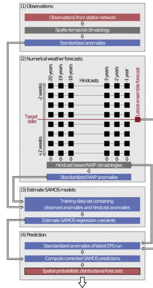
Appendix A: Standardized anomaly model output statistics (SAMOS)

For spatio-temporal ensemble postprocessing we followed the approach of Dabernig et al. (2017) and Stauffer et al. (2017b), which we summarize in the following. In contrast to other statistical postprocessing methods, SAMOS uses stan-dardized anomalies for both the response and the covari-ates. This allows one to remove location-specific and time-specific characteristics from the data and to estimate one single regression model for all stations and forecast lead times at once. For this study we closely follow the original articles (Dabernig et al., 2017; Stauffer et al., 2017b) but slightly modify the specification, especially for the temper-ature SAMOS, to adapt to the different study area.

Observation climatologies.Two separate spatio-temporal

models have been estimated for 2 m air temperature obser-vations and daily precipitation sums. Both models have ef-fects to capture seasonal, altitudinal, and spatial climatolog-ical features represented by (multi-dimensional) nonlinear functions. The 2 m temperature observations are available at an hourly temporal resolution. Therefore, additional nonlin-ear cyclic effects have to be included to capture the diurnal effects in the climatological estimates.

The spatio-temporal model for the 2 m temperature uses the geographical location (longitude lon, latitude lat, and al-titude alt), the “hour of the day” (hour), and the “day of the year” (doy) as covariates and is specified as follows:

temperature∼N _eµ_y,_eσy),

e

µ_y=f1(hour,doy,alt)

+f2(hour,doy)+f3(doy,lon,lat)

+f4(hour)+f5(doy)+f6(doy,alt)+f7(alt),

log _eσy

=g1(hour,doy,alt)+g2(hour,doy)

+g3(doy,lon,lat)

+g4(hour)+g5(doy)+g6(doy,alt)+g7(alt), (A1)

wherefqandgqare up to three-dimensional smooth spline effects. Cyclic P-splines are used for all effects depending on the “day of the year” or the “hour of the day”; all other effects use penalized thin plate splines with a varying number of possible degrees of freedom. Following the same concept, the spatio-temporal model for daily precipitation sums is defined as

precipitation1/p∼L0 eµy,eσy

,

e

µ_y=f1(alt)+f2(doy)+f3 lon,lat

+f4(doy,lon,lat),

log _eσy

=g1(alt)+g2(doy)+g3(lon,lat)

+g4(doy,lon,lat). (A2)

As for Eq. (A1), cyclic P splines are used for effects which depend on the “day of the year”, while all others use pe-nalized thin plate splines. The major difference to the tem-perature climatology (Eq. A1) is that a left-censored logistic response distributionL0is used on power-transformed

ob-servations of precipitation1/p (p=1.35; cf. Stauffer et al., 2017b). The complexity of the linear predictors in Eq. (A2) is lower than in Eq. (A1) as no effects for diurnal variation have to be considered.

Model climatology.Similar spatio-temporal climatologies

as for the observations could be estimated for all quantities from the EPS which are used as covariates in the SAMOS models. This would have to be done for each quantity sep-arately using a reasonably large data set of historical EPS forecasts. However, we instead extract the model climatolo-gies directly from ECMWF hindcasts. These hindcasts are produced operationally twice a week and consist of 10+1 members using the same model version and model specifi-cation as the current EPS. For each hindcast run the fore-casts for the same date over the most recent 20 years are computed. The hindcasts are designed to represent the cli-matology of the current EPS model and are used to cali-brate EPS forecasts and as input for postprocessing appli-cations (e.g., Hagedorn et al., 2012, 2008). For our SAMOS approach we can thus simply derive the empirical mean and empirical standard deviation over a set of hindcasts to get the climatological estimates_eµ_x and_eσx required to compute the

standardized anomalies for covariatex(Eq. 9). Climatologies for lead times when no hindcast output is available (between the regular 6 h interval) are created using simple grid-point-wise linear interpolation.

Hindcasts are produced every Monday and Thursday (available Tuesday/Friday), computed 2 weeks in advance. Taking hindcasts for±2 weeks around the date of interest yields eight independent hindcast runs with 11 members and 20 years of (re-)forecasts each, which yields 8·11·20=1760 forecasts. With this large number of independent predictions these climatological estimates are fairly robust. Due to the 4-week centered rolling window the climatologies automati-cally adapt themselves to the prevailing season. Separate cli-matologies for each forecast step are required to capture diur-nal cycles (for temperature) and to account for changes in the model climate with increasing forecast horizon such as drift-ing means or increasdrift-ing ensemble standard deviation. Thus, for this study, 13 separate climatologies for the temperature models ([+6 h,+12 h, . . .,+72 h,+78 h]) and 3 climatolo-gies for the precipitation forecasts ([+30 h,+54 h,+78 h]) are required.

Estimation of the SAMOS models (see Table 1).