University of Pennsylvania
ScholarlyCommons
Publicly Accessible Penn Dissertations
Spring 5-17-2010
Cash-Flow Risks, Financial Leverage and the Cross
Section of Equity Returns
Marcelo V. Maia
Follow this and additional works at:http://repository.upenn.edu/edissertations
Part of theFinance and Financial Management Commons
Recommended Citation
Maia, Marcelo V., "Cash-Flow Risks, Financial Leverage and the Cross Section of Equity Returns" (2010).Publicly Accessible Penn Dissertations. 161.
Cash-Flow Risks, Financial Leverage and the Cross Section of Equity
Returns
Abstract
What is the cross-sectional relationship between financial leverage and expected equity returns? How is the empirical relationship associated with firm's financial decisions? This dissertation investigates the potential explanations for the flatness relation between financial leverage and expected equity returns, and its link to firms’ capital structure determinants. Empirical evidence contradicts the theoretical prediction that leverage amplifies the equity risks. I decompose expected equity returns of book leverage portfolios according to their exposure to cash flow and discount rate risk. I find that low leverage firms have lower cash-flow beta and higher discount-rate beta than firms with high leverage. Although cash flow beta typically has a higher price of risk, book leverage portfolios load disproportionately on discount-rate beta, generating an essentially flat relation. Moreover, the main determinants of firms’ capital structures are related to firms’ sensitivities to these systematic sources of risk and have different importance for low and high leverage firms. I show that
temporary shocks are relatively more important for low leverage firms, and that financial distress risk seems to be captured by the sensitivity of firms' cash flow innovations to market discount rate news.
Degree Type
Dissertation
Degree Name
Doctor of Philosophy (PhD)
Graduate Group
Finance
First Advisor
Joao F. Gomes
Keywords
Returns Decomposition, Financial Leverage, Cash-Flow Beta, Discount-Rate Beta, Capital Structure
Subject Categories
c
COPYRIGHT
Marcelo Verdini Maia
ACKNOWLEDGMENTS
I am very grateful to my advisor, Jo˜ao Gomes. He was always patient when I
asked for help and guided me to make this work comes true. He encouraged me when
I felt exhausted. If I am able to close this cycle in my life, I owe much to him. I
am sincerely grateful to Donald Keim for teaching me important things during my
academic life at Wharton and to Dana Kiku for her kindness and invaluable advices.
I can never say enough thanks to them.
I must also thanks Andy Abel, who has always been willing to help me.
I am so grateful for the constant support from my wife, Carol. She has always
been present, specially in the most difficult moments of my life.
I am so grateful to my family, specially to my parents, to my brother, and to my
grandparents, for their support, love, and encouragement during these tough years.
Finally, I can never say enough sorry to my son, Gabriel, for my absence when he
most needed my attention. Although this time is irrecoverable, I hope it can bring to
ABSTRACT
Cash-Flow Risks, Financial Leverage and the Cross Section of Equity Returns
Marcelo Verdini Maia
Joao F. Gomes
What is the cross-sectional relationship between financial leverage and expected
eq-uity returns? How is the empirical relationship associated with firm’s financial
de-cisions? This dissertation investigates the potential explanations for the flatness
re-lation between financial leverage and expected equity returns, and its link to firms
capital structure determinants. Empirical evidence contradicts the theoretical
pre-diction that leverage amplifies the equity risks. I decompose expected equity returns
of book leverage portfolios according to their exposure to cash flow and discount rate
risk. I find that low leverage firms have lower cash-flow beta and higher discount-rate
beta than firms with high leverage. Although cash flow beta typically has a higher
price of risk, book leverage portfolios load disproportionately on discount-rate beta,
generating an essentially flat relation. Moreover, the main determinants of firms
cap-ital structures are related to firms sensitivities to these systematic sources of risk
and have different importance for low and high leverage firms. I show that temporary
shocks are relatively more important for low leverage firms, and that financial distress
risk seems to be captured by the sensitivity of firms’ cash flow innovations to market
Contents
1 Introduction 1
2 Related Literature 6
3 Empirical Framework 12
3.1 Return Decomposition . . . 12
3.2 Traditional Vector Autoregressive Implementation . . . 13
3.3 Alternative Implementations . . . 17
4 Data and Results 20
5 Determinants of Risk Exposures and Capital Structure 37
6 Concluding Remarks 45
Appendix: Variable Definition 48
List of Tables
4.1 Summary Statistics . . . 22
4.2 Excess Returns for Book Leverage Portfolios . . . 24
4.3 Aggregate VAR Estimates . . . 26
4.4 Cash Flow and Discount Rate Betas for Book Leverage Portfolios . . 27
4.5 Cash Flow and Discount Rate Betas for Book Leverage and Book to Market Portfolios . . . 29
4.6 Firm Level VAR estimates . . . 31
4.7 Four Beta Decomposition . . . 33
4.8 Long Run Risk Implementation . . . 35
4.9 Direct Proxies Implementation . . . 36
5.1 Determinants of Betas and Capital Structure . . . 41
Chapter 1
Introduction
The idea that financial leverage should be positively related to equity returns dates
back to Modigliani-Miller’s (1958 and 1961) famous Proposition II. This is an
ele-mentary notion in finance, where equity risk is formed by two fundamental risks:
operating risk and financing risk. Given operating risk, average returns are
increas-ing in leverage. That is, financial leverage amplifies the exposure of equities to priced
systematic risks.
However, many empirical papers document that raw returns have a negative, or
at least flat, relation with financial leverage, and that returns adjusted by traditional
sources of risks have an even stronger negative relation with leverage.
These findings are usually seen as a puzzle. However, it is possible that market
frictions lead low leverage firms to have greater exposures to systematic risks. For
example, firms might optimally choose low leverage in response to greater exposure
to systematic risks. Then, the amplification effect of leverage on equity risk could
be either attenuated or dominated1. Consequently, identifying economic sources of
risk that justify the empirical evidence concerning the relation between leverage and
returns is an important issue and can help understand firms’ financial decisions.
The importance for investors of two sources of risk in the economy has been
a topic of intense study in the asset pricing literature. Specifically, Campbell and
Vuolteenaho (2004) argue that investors care about the permanent effects of future
market’s cash flow innovations and the transitory effects of the market’s discount
rate innovations. Bansal and Yaron (2004) show that investors care about long-run
growth prospects and the level of economic uncertainty, and that changes in these
fundamentals drive the risks in asset prices. Among other implementations, both
approaches are successful in explaining the cross-sectional dispersion in asset prices
and provide two distinct measures of systematic risk, usually called cash flow risk and
discount-rate risk.
The main goal of this dissertation is to investigate empirically what can explain
this puzzling cross-sectional relation between leverage and equity returns. Specifically,
I argue that the flat (or sometimes negative) relation is a natural outcome of the
association between firms’ cash flow innovations and two distinct sources of systematic
risk described above.
In fact, since firms’ cash flow prospects are important for capital structure
de-cisions, different shocks affecting firms’ cash flows should also matter to determine
capital structure of firms.
Although a capital structure decision is fundamentally important for stockholders’
risk, leverage usually has not been considered as an important firm characteristic in
the asset pricing literature. Papers generally concentrate on size, book-to-market,
and industry portfolios since that these sorts produce economically meaningful risk
infor-mation contained in leverage2. However, it has been argued recently3 that financial
leverage is at the root of why size and book to market matter.
This work makes several contributions. First, I calculate the return sensitivities
of portfolios sorted based on book leverage to the market cash flow and discount rate
news. To do so, I implement the framework proposed by Campbell and Vuolteenaho
(2004), through the use of the vector auto-regressive (VAR) approach. I find that
firms with low leverage have lower cash-flow beta and higher discount-rate beta than
firms with high leverage. Although cash flow beta typically has a higher price of risk,
book leverage portfolios load disproportionately on discount-rate beta, generating an
essentially flat relation between leverage and returns.
The amplification effect of leverage on equity risk, which comes naturally from
the textbook intuition, seems to be dominated by greater exposure to systematic risk
and different sensitivities of firms’ returns should reveal information not captured by
the single CAPM beta. In fact, for high leverage firms, both shocks may have roughly
the same importance and, for low leverage firms, cash-flow beta is essentially zero.
To better characterize the association between leverage and cash-flow and
discount-rate betas, I further decompose firms’ return innovations into cash flow news and
discount rate news, and calculate sensitivities of each firm’s components to market
news. I find that the high betas of low leverage stocks with the market’s discount rate
shocks and the high betas of high leverage firms with the market’s cash flow shocks are
determined by the properties of their cash flows. Specifically, the covariation between
firm’s news about cash flows and market innovations explains the positive relation
between leverage and cash-flow beta and the negative relation between leverage and
2E.g., Chan and Chen (1991); Fama and French (1992); Chen and Zhang (1998)
discount rate beta.
The heterogeneity in betas among firms with different capital structures appears
to be related with the effect of the type of systematic shocks on their cash flows.
So, beyond the importance of earnings prospects for financial decisions, the effect of
different shocks on cash flows might have important consequences on capital structure
choices.
Usually, capital structure theory focuses on idiosyncratic risk to explain corporate
financial decisions. For example, trade-off theory argue that firms with more volatile
cash flows face higher expected costs of financial distress and should use less debt.
More volatile cash flows reduce the probability that tax shields will be fully utilized,
implying that higher risk should result in less debt. In contrast, this dissertation
analyzes empirically how systematic risk is associated with capital structure decisions
by investigating the relation between variables successfully used as leverage predictors
and cash-flow betas.
I use sectional firm-level regressions to identify whether the traditional
cross-sectional leverage predictors are related with the different betas. That is, I study the
determinants of risk exposures and their links to capital structure decisions on the
entire sample and on the two extreme low and high leverage portfolios betas.
I use a parsimonious list of factors considered to have some influence on corporate
leverage. This includes the variables proposed by Frank and Goyal (2007b). Also, I
include both capital expenditures, as an alternative proxy for growth, and probability
of default, to be extensively used as a direct proxy related to financial distress risk.
The final set of variables is hence composed of profitability (ROA), unlevered z-score,
tangibility, capital expenditures (capex), firm size, and book-to-market.
temporary, sometimes high, shocks to market discount rate. This effect is pervasive
for both extreme portfolios, but more pronounced for low leverage firms.
Furthermore, considering that a decrease in financial distress risk is associated
both with lower probability of default and with more tangible assets, and that both
underinvestment problem and asset substitution are more evident when firms go
to-ward distress, the findings indicate that the sensitivity of firms’ cash-flows to market
discount-rate news is capturing exactly this risk, which is more pronounced for low
leverage firms. In fact, probability of default matters only for low leverage firms, the
effect of tangibility on risk is twice as higher than for high leverage firms, and the
effects of book-to-market changes only affect low leverage firms.
Finally, I find that cash-flow shocks have relatively more importance for low
lever-age. Taking together, the results suggest that firms choose their capital structure in
response to the systematic risks they face.
The rest of the dissertation is organized as follows. Chapter 2 briefly reviews
the related literature. Chapter 3 presents the empirical framework that form a basis
for this work. Chapter 4 contains descriptions of the data and results, showing how
book leverage is related to cash-flow and discount rate risk. Chapter 5 presents the
determinants of different betas and their link to capital structure factors. Chapter 6
Chapter 2
Related Literature
This dissertation is related with studies that have directly examined the relationship
between financial leverage and stock returns. This literature started with two seminal
papers that are concerned primarily with the implications of Modigliani and Miller
(1958 and 1961) proposition II.
Bandhari (1988) was the first study to investigate this proposition. He found
that market leverage is positively related to expected equity returns, confirming the
increasing in risk associated with high leverage. Fama and French (1992) also
docu-mented that market leverage is positively related to expected equity returns. In
con-trast, when book leverage is used as proxy, it is negatively related to equity returns,
the so called financial leverage puzzle. However, Fama and French (1992) argue that
book leverage captures both the effect of size and the effect of book-to-market. This
claim relegated leverage to the second plan in the asset pricing literature, motivating
follow-up papers to focus exclusively on size and book-to-market.
Recently, researchers looked more closely to the effects of financial leverage on
equity returns. On the empirical side, Korteweg (2004) takes a time series approach
and shows that, among firms performing exchange offers, equity factor loadings for
trading strategy, involving firms with extreme levels of financial leverage. This result
deepens the financial leverage puzzle and raises the question of why this happens.
Penman et al. (2006) take an accounting approach to test the relation between
financial leverage and expected equity returns. They separate the leverage component
of the book-to-market ratio pertaining to financing risk from the component that
pertains to operations and observe an anomalous effect with respect to the leverage
component.
Obreja (2007) builds his idea from the implications of Fama and French (1992)
for the relation between book leverage and equity returns. He asks whether leverage
contains information above and beyond size and book-to-market equity. The paper
brings a structural model where the relative distribution of assets in place and growth
options is the main determinant of equity risk premia. For all-equity-financed firms,
this distribution can be summarized in terms of firm-specific productivity and two
firm variables, namely book-to-market equity and firm size, but for firms financed
with both equity and debt, this distribution depends also on financial leverage.
Firm size and book-to-market equity cannot capture the cross-sectional variation
in equity returns due to financial leverage. Leveraged firms are riskier because they
are stuck with too much capital, during times of low productivity. These firms cannot
scale down production without increasing the likelihood of default. The model can
generate qualitatively and, sometimes, quantitatively the cross-sectional properties
of equity returns associated with firm characteristics such as book-to-market equity,
firm size, market leverage, book leverage and debt/equity ratio.
George and Hwang (2009) also document that the relation between leverage and
returns is negative. They build a simple model specified to solve the distress and
distress costs. They hypothesize that low (high) leverage can be used as an indicator
of exposure to greater (lesser) financial distress costs. This implies that if financial
distress risk is priced with a return premium for high cost firms, then expected returns
will be higher for low leverage firms than for high leverage firms.
Gomes and Schmid (2009) propose a theoretical interpretation for the apparently
contradictory empirical evidence. Because of the endogenous relation between
lever-age and investment, high leverlever-age firms in their model tend to be more mature firms
with more book assets and fewer growth opportunities; that is, they should produce
less risk. A coherent parametrization of their model can replicate the actual relation.
Also, using a real options model, they show that firms’ equity beta only increases with
financial leverage in a static world in which leverage is exogenously determined1.
I add to this debate by documenting that the empirical relation between book
leverage and stock returns is flat, and arguing that firms with different leverage ratios
have different exposures to the market’s systematic risks. Also, I document that the
different sensitivities to market news are implied by the characteristics of firms’
cash-flows. Moreover, these different sensitivities are determined by factors extensively
studied in the capital structure literature.
This study is also related to the return decomposition literature, which focuses
on understanding the systematic risks affecting stock returns. Although most of this
literature is concerned in developing new implementations to explain asset pricing
anomalies (Campbell and Vuolteenaho (2004), Campbell et al (2009), Chen and Zhao
(2009a, 2009b), Da and Waracka (2009), Bansal, Dittmar, and Lundblad (2004)),
here I am interested in understanding how cash-flow and discount-rate sensitivities
1Nielsen (2006) study the relationship between companies’ choice of capital structure and their
are related to book leverage by applying the predictions of a standard framework.
Although the spread between low and high leverage portfolios seems not to be large
enough to be interesting for an asset pricing perspective, the flat (negative) relation
constitutes a puzzle and should be informative about underlying factors affecting
capital structure decisions.
It has been documented in the asset pricing literature that investors are
funda-mentally concerned with two sources of risk in the economy. In fact, since stocks
are priced by discounting their expected future cash flows, it is natural to think that
movements in stock prices are driven both by news about cash flows and discount
rates. Therefore, understanding how economic fundamentals drive these changes is
of crucial importance.
Campbell and Vuolteenaho (2004) argue that investors care (more) about the
permanent effects of future market’s cash flow innovations and the transitory effects
of market’s discount rate innovations. Specifically, the required return on a stock
is determined not by its overall CAPM beta, but by two separate betas, one with
permanent shocks to market cash flows (cash-flow beta), and other with temporary
shocks to market discount rates (discount-rate beta). They show, for example, that
the high average return on value stocks is predicted by the two-beta model2 .
Bansal and Yaron (2004) demonstrate that investors care about long-run growth
prospects and the level of economic uncertainty, and that changes in these
fundamen-tals drive risks in asset prices. Current shocks to expected growth alter expectations
concerning future economic growth not only in the short run but also for the very
long run. Also, they argue that time variation in expected excess returns is due to
2Koubouros, Malliaropulos, and Panopoulou (2005) extend the approaches of Campbell and
variation in economic uncertainty.
Bansal, Dittmar, and Lundblad (2002 and 2004) study Bansal and Yaron’s
impli-cations for the cross-sectional differences in mean returns across assets. They show
that systematic risks in cash flows can account for the cross-sectional differences in
risk premia of assets, accounting for the puzzling value, size, and momentum spread
in the cross section of assets.
All of these approaches are based on the return decomposition framework, differing
only in their implementation. Campbell and Vuolteenaho (2004) explore the return
predictability. On the other hand, Bansal, Dittmar and Lundblad (2004) explore the
cash flow (dividends) predictability.
Finally, this paper contributes to the empirical capital structure literature
con-cerned with studying the cross-sectional differences in financial leverage. As
sum-marized by Frank and Goyal (2007a and 2007b), the study of the determinants of
capital structure is of fundamental importance because reliable factors explain only
25% of firms’ heterogeneity. The contribution of this dissertation is to suggest that
different cash-flow sensitivities to market innovations seem to add to possible
explana-tions of what determines the heterogeneity of firms’ capital structure, guiding future
development in this literature.
There are some papers which share their ideas with this dissertation. First,
Hack-back, Miao, and Morellec (2006) contend that macroeconomic conditions should have
a large impact not only on credit risk but also on firms financing decisions. Indeed, if
one determines optimal leverage by balancing the tax benefit of debt and bankruptcy
costs, then both the benefit and the cost of debt should depend on macroeconomic
conditions. The tax benefit of debt obviously depends on the level of cash flows,
contraction. In addition, expected bankruptcy costs depend on the probability of
default and the loss given default, both of which should depend on the current state
of the economy. As a result, variations in macroeconomic conditions should induce
variations in optimal leverage. The purpose of their paper is to provide a first step
to-wards understanding the quantitative impact of macroeconomic conditions on credit
risk and capital structure decisions.
Recently, two other papers explore theoretically the effects of different shocks on
firm’s cash flows and their implication for capital structure decisions. Chen (2009)
in-troduces macroeconomic conditions into firms’ financing decisions and builds a
struc-tural model showing how business cycles affect financing decisions and the pricing of
corporate securities. Gorbenko and Strebulaev (2009) investigate corporate financial
policies in the presence of both temporary and permanent idiosyncratic shocks to
cash flows, and show that temporary shocks seem to be more important to explain
empirical stylized facts about corporate financial decisions.
This dissertation similarly finds that different systematic risks on firm’s cash flows
might be informative about capital structure decisions, providing empirical evidence
for these papers and directly investigating how the effect of shocks to firm’s cash flows
Chapter 3
Empirical Framework
3.1
Return Decomposition
Starting from the accounting definition of asset returns, Campbell and Shiller (1988)
and Campbell (1991)1show that log returns can be decomposed into two components:
rt+1−Etrt+1 = (Et+1−Et) X
ρj∆dt+1+j−(Et+1−Et) X
ρjrt+1+j =NCF,t+1−NDR,t+1
(3.1)
wherert+1 is a log stock return,dt+1 is the log dividend paid, ∆ denotes a one period
change,Etdenotes a rational expectation at time t,ρis a discount coefficient,NCF,t+1
denotes cash flow news, andNDR,t+1denotes discount rate news (or expected returns).
This decomposition is an identity and holds independent of the underlying model
for expected returns. It shows that unexpected stock returns must be associated with
changes in expectations for future cash flows and/or discount rates. An increase in
expected future cash flows is associated with a capital gain today, while an increase
in discount rates is associated with capital loss today.
It can be demonstrated empirically that these two components display substantial
volatility and are not highly correlated with one another. This finding allows using
the return decomposition to construct different measures of stocks’ systematic risks.
That is, if equation (3.1) is used to decompose aggregate market returns, the CAPM
beta is given by the sum of two betas, the market cash-flow beta and the market
discount-rate beta, respectively:
βi,CFM =
Cov(ri,t, NCFM,t) V ar(re
M,t−Et−1rM,te )
(3.2)
βi,DRM =
Cov(ri,t,−NDRM,t) V ar(re
M,t−Et−1rM,te )
(3.3)
where βi,M =βi,CFM +βi,DRM.
Although the sum of the market cash-flow beta and the market discount-rate beta
is equal to the CAPM beta, they carry different risk premia, providing two potentially
different sources of risk. From ICAPM, one can show that:
Et[Ri,t+1]−Rf,t+1 =γσM,t2 βi,CFM,t +σ 2
M,tβi,DRM,t, (3.4)
where γ is the investor’s coefficient of risk aversion and σ2M is the variance of the
aggregate market returns.
3.2
Traditional Vector Autoregressive
Implemen-tation
How to implement the calculation of these betas is still a topic on intense debate, since
the news components are not directly observable. Here I follow the implementation
of Campbell and Vuolteenaho (2004) and Campbell et al (2009) both of whom use
the vector autoregressive (VAR) approach to disentangle cash-flow and discount-rate
shocks at market and firm levels. They build on the fact that returns are predictable
and one only needs to understand their dynamics, not the short-run dynamics of
Chen and Zhao (2009) question this implementation, offering arguments showing
that it is not quite robust. It is not my intention to take a side in this disagreement.
To alleviate any concerns about the validity of my results, I also implement the
calculation of betas using alternative measures commonly seen in the literature.
The first step, then, is to decompose the CAPM beta by calculating market cash
flow and discount rate news. The VAR methodology first estimates the termsEtrt+1
and NDR,t+1 and then usesrt+1 and equation (3.1) to back out the cash flow news.
Specifically, one can assume that the data are generated by a first-order VAR
model
zt+1 =a+ Γzt+ut+1 (3.5)
where zt+1 is aN-by-1 state vector with rt+1 as its first element,a and Γ areN
-by-1 vector and N-by-N matrix of constant parameters, and ut+1 is an i.i.d N-by-1
vector of shocks. Thus:
NDR,t+1 = e10λut+1 (3.6)
NCF,t+1 = (e10+e10λ)ut+1 (3.7)
where λ≡ρΓ(I−ρΓ)−1 and e1 is the canonical vector.
Campbell and Vuolteenaho (2002) argue that returns generated by cash-flow news
are never reversed subsequently, whereas returns generated by discount rate news are
offset by lower returns in the future. That is, the two beta decomposition suggests
that there are both a permanent (or long-run) risk and a transitory (or short-run) risk
not captured by the single CAPM beta. Therefore, conservative long-term investors
are more concerned with cash-flow risk than with discount rate risk. In other words,
exclusively, important, and, in general, returns should be positively related to
cash-flow beta, as derived in equation (3.4). The relevance of this method is the possibility
of extracting two different movements in the market dynamics that could potentially
affect firms’ returns, and that were potentially hidden in the single CAPM beta.
Note that this implementation only decomposes the market return into two
com-ponents. This decomposition generates the broad definition of cash-flow and
discount-rate beta. To better understand firms’ sensitivities to market innovations, it is
neces-sary to investigate whether and how firms’ components are related to the two market
sources of risk. Specifically, I follow the approach of Campbell, Polk and Vuolteenaho
(2009) and further decompose each firm’s returns into their two news components.
That is:
ri,t+1−Etri,t+1 = (Et+1−Et) X
ρj∆di,t+1+j−(Et+1−Et) X
ρjri,t+1+j =Ni,CF,t+1−Ni,DR,t+1
(3.8)
The following four betas can thus be defined:
βCFi,CFM =
Cov(NCFi,t, NCFM,t) V ar(re
M,t−Et−1reM,t)
(3.9)
βCFi,DRM =
Cov(NCFi,t,−NDRM,t) V ar(re
M,t−Et−1reM,t)
(3.10)
βDRi,CFM =
Cov(NDRi,t, NCFM,t) V ar(re
M,t−Et−1reM,t)
(3.11)
βDRi,DRM =
Cov(NDRi,t,−NDRM,t) V ar(re
M,t−Et−1reM,t)
(3.12)
There is some confusion about how to denominate these six betas. Many papers
call βCF i,CF M cash-flow risk, because they only focus on understanding its relevance
for pricing. To avoid confusion, I use the following nomenclature. βCFi,CFM:
cash-flow risk, and βDRi,DRM: Discount rate discount rate risk. Then, equations (3.9)
and (3.10) define the two firms’ cash-flow risks, and equations (3.11) and (3.12) define
firms’ discount rate risks. Finally, cash-flow beta and discount-rate beta are defined
as follows:
βi,CFM =βCFi,CFM +βDRi,CFM (3.13)
βi,DRM =βCFi,DRM +βDRi,DRM (3.14)
It must be noted that the widespread use of these two (four) beta decompositions
serves to explain the apparent anomalies posed by value, small and momentum stocks.
In regard to these stocks, a large spread between returns of extreme portfolios and
an inverse relation to market beta generates an asset pricing puzzle, constituting a
potential interesting research topic itself. Leverage has not been a subject of study
in the asset pricing literature because sorts based on book leverage do not produce
meaningful risk premia. Moreover, some papers argue that size and book-to-market
capture information contained in leverage.
However, what I am examining here is the puzzling fact that, although financial
leverage is a fundamental characteristic of a firm, the object of an optimal decision
by management, it apparently plays an innocuous role in increasing equity risks, as
firms become more leveraged.
Thus, it seems interesting to analyze how leverage is associated with market cash
flow and discount rate risks. Indeed, when firms gear up, shocks affecting their
cash flows become even more important for capital structure decisions. Recall that
each market news component should be capturing different systematic risks, which
3.3
Alternative Implementations
The VAR methodology used to implement the calculation of both firms’ and market
news allows calculating the effect of today’s shocks over the discounted infinite future,
capturing the correct effect from changes in investors’ expectations of prices and
returns. However, as discussed above, the best implementation method is still under
debate.
To alleviate any concern about the results obtained in the last section, I use
alter-native measures to estimate cash-flow and discount-rate betas: long run risk model
(as in Bansal, Dittmar, and Lundblad (2004)), as well as direct methods. I choose
proxies used extensively in the literature that have proved successful in explaining
the facts under consideration.2 It should be noted that the methods developed in
the literature do not completely determine the two (four) betas. For example, the
long-run risk model implemented in this dissertation (Bansal et al. (2004)) focuses
on what they called cash-flow betas (sensitivities of firms’cash flow innovations to
market cash flow news).
The long run risk model explores the fact that cash-flows seem to be better
pre-dicted than returns. This model differs from the method used in this paper in
estimat-ing first discount rate news. The VAR methodology is used to estimate directly cash
flow news. The original implementation assumes that the de-meaned log consumption
growth follows a simple AR(1):
gc,t =ρcgc,t−1 +ηt (3.15)
2It is not the main goal of this dissertation provides an extensive implementation of these
with ηt being the consumption news at date t, and gc,t is the de-meaned log
consumption growth.
Further, it is assumed that the relationship between de-meaned dividend and
consumption growth rate is:
gi,t =φi( 1
K
K X
k=1
gc,t−k) +ui,t (3.16)
ui,t = L X
j=1
ρj,tui,t−j +εi,t (3.17)
Thus, equations (3.15), (3.16), and (3.17) are mapped into a VAR(1), and in a
algebraic process similar to the one that generated equations (3.6) and (3.7), one can
represent the innovation to current and expected future cash-flow growth rates. The
exposure of this innovation to consumption growth is the firms’ cash flow innovation
to consumption growth.
I use a method similar to this one. Instead of using the VAR method, the
sensi-tivities of portfolios’ cash flow innovation to market cash flow news is given by:
N X
j=1
ρjgi,t+j,j+1 =α+βCF i,CF M N X
j=1
ρjgM,t+j,j+1+ (3.18)
where gi,t+j,j+1 is the log de-meaned dividend growth for portfolio i at date t+j.
The measurement of dividends for each portfolio is the following. From the
ac-counting definition of returns, we have:
Ri,t =hi,t+1+yi,t+1 (3.19)
portfolio i, the level of dividends is:
Di,t+1 =yi,t+1Vi,t (3.20)
Vi,t+1 =hi,t+1Vi,t (3.21)
where V0 = 1, Di,t+1 is the total cash dividends paid out by a portfolio at time t
that extracts the dividends and reinvests the capital gains.
The direct methods use the portfolio-level accounting return on equity (ROE) as
a proxy for cash flows. Campbell, Polk and Vuolteenaho (2009) and Cohen, Polk, and
Vuolteenaho (2003, 2009) argue that the discounted sum of ROE is a good measure
of firm-level cash-flow fundamentals. Thus, a ROE-based proxy for portfolio level
cash-flow news is the following:
Ni,CF,t+1 =
N X
j=1
ρj−1roei,t,t+j (3.22)
where roei,t,t+j is the log of real profitability for portfolio i, sorted in year t, and
measured in year t+j.
To proxy for discount-rate news at the market level, I use the proxy derived in
Campbell, Polk and Vuolteenaho (2009):
−NM,DR,t+1 =
N X
j=1
[ρj−1∆t+jln(P/E)M] (3.23)
To emphasize log term trends in cash flows, I examine horizons (N) from two to
Chapter 4
Data and Results
The primary data and the methodology of variable construction are quite standard.
Data is obtained from CRSP and Compustat. Monthly returns and market
capital-ization are from CRSP, and financial information and other firms’ characteristics are
from the CRSP/Compustat merged database. Observations with missing values for
variables used directly in the study are excluded. Financial and utilities industry are
excluded, as are stocks of firms with non-positive book value of equity and/or
nega-tive total liabilities. Moreover, to eliminate likely data errors, I discard those firms
with book-to-market (BE/ME) lower than 0.01 and greater than 100 at the time of
the sort.
To correct for survival bias, I only include stocks that have been in Compustat
for more than two years, and restrict the sample to common stocks. When necessary,
I describe any change in the data, in the sample and in the implementation used.
Variable construction and other details can be found in the appendix.
This work studies risk characteristics of portfolios sorted by book leverage. I
choose book leverage as a proxy for financial leverage primarily because book leverage
seems to capture the endogenous decision of managers about capital structure1.
mechan-The construction takes place as follows. Portfolios are formed on July 1st every
year (t) and run through June 30th of the next year (t+ 1) based on Compustat
and CRSP data for each firm as of December of the previous year (t −1). Book
leverage portfolios are created by sorting on NYSE stocks only and then using the
break points for all NYSE, Amex and NASDAQ stocks. I use monthly value-weighted
excess returns (over 30 day T-bill) averaged over all months and years. I included the
bias correction for delisted firms suggested by Shumway (1997) and Shumway and
Warther (1999).
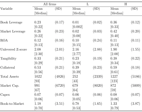
Table 4.1 shows some characteristics of these portfolios. To save space and to focus
on the differences between low and high leverage firms, statistics are only shown for
all firms and for the two extreme portfolios. A quick look reveals several unsurprising
differences. High leverage firms tend to be larger (both by book value of assets
and market capitalization), have fewer growth opportunities (i.e., higher
book-to-market), have more tangible assets, have more collateral, invest more and have higher
probability of default. It is interesting to note, however, that both portfolios tend to
have similar returns on assets (dividends are roughly the same for these portfolios).
In panel A of table 4.2, I document that the relation between excess returns and
book leverage is essentially flat, confirming the results of past empirical studies. The
average difference between returns of the two extreme portfolios is only 0.02% and
statistically insignificant. This result is at odds with traditional theories. Intuitively,
financial leverage amplifies the exposure of equity to priced systematic risks, so
finan-cial leverage should be positively related to stock returns
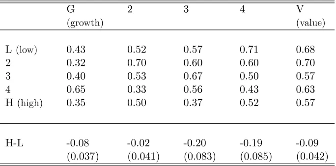
In addition to this, I provide evidence that excess returns of portfolios sorted
by book leverage and book-to-market also are inversely related to financial leverage,
Table 4.1: Summary Statistics
The sample consists of all nonfinancial, non-utility firms in the Compustat database from 1965 to 2006. The table presents variable averages, medians (in brackets), and standard deviations (SD) for the entire sample (All Firms), as well as the subsample of firms for the extreme lowest (L) and highest (H) book leverage portfolios. The variable definitions are provided in the Appendix.
All firms L H
Variable Mean (SD) Mean (SD) Mean (SD) [Median] [Median] [Median]
Book Leverage 0.23 (0.17) 0.01 (0.02) 0.36 (0.12)
[0.22] [0.002] [0.33]
Market Leverage 0.26 (0.23) 0.02 (0.03) 0.42 (0.20)
[0.22] [0.00] [0.40]
ROA 0.12 (0.16) 0.10 (0.24) 0.11 (0.11)
[0.13] [0.15] [0.13]
Unlevered Z-score 2.08 (2.01) 2.16 (2.88) 1.90 (1.55)
[2.30] [2.77] [2.00]
Tangibility 0.33 (0.21) 0.23 (0.19) 0.38 (0.22)
[0.29] [0.18] [0.34]
Collateral 0.53 (0.21) 0.39 (0.23) 0.59 (0.18)
[0.56] [0.39] [0.61]
Total Assets 1022 (4826) 252 (2339) 1227 (5186)
[93] [43] [123]
Market Cap. 991 (6720) 679 (8020) 872 (5009)
[67] [64] [59]
Capex 0.07 (0.07) 0.06 (0.06) 0.08 (0.07)
[0.06] [0.05] [0.06]
Book-to-Market 1.18 (3.51) 0.78 (1.65) 1.33 (3.87)
confirming the evidence presented in George and Hwang (2009) and Penman et al.
(2006). They demonstrate that book-to-market is not able to capture all of the
infor-mation contained in leverage, and that, if one controls the return by risks extracted
using the standard Fama-French model, the inverse relation becomes even stronger.
To derive the cash-flow and discount rate betas, we need to estimate the market’s
cash flow and discount-rate innovations, as in equations (3.6) and (3.7). To
opera-tionalize the VAR method, the literature assumes that the vector z is composed of
four state variables chosen by their power and by their success in predicting future
returns. They are the excess market return, the yield spread between long-term and
short-term bonds, the market’s smoothed price-earnings ratio, and the small-stock
value spread, measured as the difference between the log(Book Equity/Market
Eq-uity) of the small high-book-to-market portfolio and the log(Book Equity/Market
Equity) of the small low-book-to-market portfolio.
Shortly, the intuition for these variables is the following. The yield curve tracks
the business cycle. High price-earnings ratios will necessarily imply low long-run
expected returns, if expected earnings growth is constant. If small growth stocks
have low expected returns and small value stocks have high expected returns, and
this return differential is not explained by the CAPM betas, the ICAPM requires the
small growth stock returns to predict lower future market returns and small value
stocks returns to predict higher future market returns.
For the VAR estimation, I use monthly observations for returns and state variables
covering the period between 1929:1 to 2006:12. The data for VAR implementation
is taken from John Campbell’s website (which covers the period between 1929:1 to
2001:12) and extended to 2006:12. I have also estimated this VAR for the shorter
Table 4.2: Excess Returns for Book Leverage Portfolios
The sample consists of all nonfinancial, non-utility firms in the annual Compustat database between 1965 and 2006. Prices, shares outstanding and returns are from CRSP. The table presents excess returns, in percentage points, calculated as the monthly average of value-weighted portfolio returns in excess of 30 day T-bill rates. L represents the portfolio with the lowest book leverage, H represents the portfolio with the highest leverage, G represents the growth portfolio, and V represents the value portfolio. In panel A, portfolios are formed by a single sorting based on book leverage. In panel B, portfolios are formed by a double sorting based on book leverage and book-to-market. Standard errors are in parentheses. All variables are defined in the Appendix.
Panel A: Excess Returns for Portfolios Sorted Based on Book Leverage
L 2 3 4 H H-L
Excess Return 0.49 0.53 0.55 0.55 0.51 0.02 (0.046)
Panel B: Excess Returns for Portfolios Sorted Based on Book Leverage and Book-to-Market
G 2 3 4 V
(growth) (value)
L (low) 0.43 0.52 0.57 0.71 0.68
2 0.32 0.70 0.60 0.60 0.70 3 0.40 0.53 0.67 0.50 0.57 4 0.65 0.33 0.56 0.43 0.63
H (high) 0.35 0.50 0.37 0.52 0.57
to recover market news, I decided to make use of data availability to extract all
information. The estimation does not alter the results, which are available upon
request2.
The right choice of these variables is essential for the VAR implementation to be
correct. Chen and Zhao (2009) estimate several other reasonable VARs that imply
lower bad betas for value stocks than for growth stocks, exactly the opposite of
Campbell and Vuolteenaho’s (2004) results, casting doubt on the validity of their
approach.
Specifically, Chen and Zhao show that value stocks have lower bad betas than do
growth stocks in recent data if a valuation ratio is excluded from the VAR system,
or if the log price-smoothed earnings ratio is replaced by either the log price-earnings
ratio using current one-year earnings without smoothing, the level of the
dividend-price ratio or the level of the book-to-market ratio. Campbell et al. (2009) comment
on their results and observe, among other things, that Chen and Zhao’s specifications
merely verify Campbell and Vuolteenaho’s (2004) report that a VAR system must
include an aggregate valuation ratio with predictive power for the aggregate market
return if it is to generate a higher bad beta for value stocks than for growth stocks.
That is, for the VAR approach to be successful, one must use the state vector described
above.
Table 4.3 reports parameter estimates for the aggregate VAR model. The
magni-tudes and significance of each parameter are consistent with previous findings in the
literature and were extensively discussed in Campbell and Vuolteenaho (2004). The
first row of the table shows that all four VAR state variables have some ability to
2Campbell and Vuolteenaho (2004) provides many robustness checks for this VAR
Table 4.3: Aggregate VAR Estimates
This table shows the OLS parameter estimates for a first-order VAR model including a constant, the log excess market return (RM), term yield spread (TY), price-earnings ratio (PE), and small-stock value spread (VS). Each pair of rows corresponds to a different dependent variable. The first five columns report coefficients on the five
explanatory variables, and the remaining column show R2 statistics. OLS standard
errors are in brackets. The sample period for the dependent variables is 1929:1-2006:12, comprising 935 monthly data points.
constant RM,t T Yt P Et V St R2(%)
RM,t+1 0.064 0.095 0.005 -0.016 -0.011 2.51
[0.019] [0.032] [0.003] [0.005] [0.005]
T Yt+1 0.040 -0.003 0.911 -0.020 0.048 85.15
[0.095] [0.160] [0.013] [0.025] [0.026]
P Et+1 0.023 0.516 0.001 0.992 -0.003 99.07
[0.013] [0.021] [0.002] [0.003] [0.004]
V St+1 0.018 0.001 -0.000 -0.002 0.992 98.44
[0.017] [0.028] [0.002] [0.004] [0.005]
predict excess returns on the aggregate stock market.
In table 4.4, the betas are calculated for single sorted portfolios based on book
leverage, revealing that high leveraged stocks have higher cash-flow betas than low
leveraged stocks, but lower discount-rate betas. The difference in cash-flow betas
between the extreme portfolios is 0.091 and statistically significant. On the other
hand, discount-rate betas are higher for low leverage stocks than for high leverage
stocks. The difference between the extreme portfolios is economically large (-0.27)
Table 4.4: Cash Flow and Discount Rate Betas for Book Leverage Portfolios
The table reports cash flow and discount rate betas using market innovationsNM,CFt+1
and NM,DRt+1 extracted using the estimates of the aggregate VAR. The sample
consists of all nonfinancial, non utility firms in the annual Compustat database between 1965 and 2006. Prices, shares outstanding and returns are from CRSP.
βi,CF M =
Cov(ri,t+1,NM,CFt+1)
V ar(rM,t+1) and βi,DRM =
Cov(ri,t+1,NM,−DRt+1)
V ar(rM,t+1) . In panel A, quintile
portfolios are formed each year by sorting firms on year t book leverage. The portfolio i=L is the extreme low leverage portfolio and i=H is the extreme high leverage port-folio. H-L represents the difference between extreme high and low leverage portfolios. The standard errors are in parentheses, estimated using the Newey-West method with five lags.
L 2 3 4 H H-L
βi,CF M (Cash-Flow Beta) -0.007 0.045 0.065 0.078 0.084 0.091 (0.03) (0.025) (0.026) (0.027) (0.024) (0.03)
true that, for every portfolio formation based on firms’ characteristics one needs to
obtain the same pattern, as one might suspect. Specifically, other studies report
similar patterns to those obtained here for portfolios sorted on size and
book-to-market, and argue that the results help to explain common asset pricing anomalies.
It is possible to produce, for example, a spread only in discount-rate betas but
no spread in cash-flow betas, for portfolios sorted on past market beta. The former
portfolio formation creates the same flat pattern in returns as does book leverage
sorting.
Second, although cash flow risk typically has a higher price of risk, book leverage
portfolios load disproportionately on discount-rate beta, generating an essentially
flat relation between leverage and returns. This result suggests that the amplification
effect of leverage on equity risk, which comes naturally from the textbook intuition,
seems to be dominated by greater exposure to systematic risks.
In fact, different sensitivities of firms’ returns might reveal information not
cap-tured by the single CAPM beta, and the flat relation between financial leverage and
expected equity returns is more informative than suspected so far. Indeed, as already
noticed before, cash-flow beta seems to capture permanent (or long run) effects on
returns, and discount rate beta seems to capture transitory (or short-run) effects on
returns. Hence, two interesting facts should be observed. First, for higher leverage
firms, cash-flow betas have an increasing importance, tending to have the same
impor-tance as discount-rate beta (depending on the value of the coefficient of risk aversion).
That is, they suffer both from transitory shocks and from permanent shocks. Second,
for low leverage firms, cash-flow beta is essentially zero. That is, only temporary
shocks in the economy matter for those firms.
Table 4.5: Cash Flow and Discount Rate Betas for Book Leverage and Book to Market Portfolios
The table reports cash flow and discount rate betas using market innovationsNM,CFt+1
and NM,DRt+1 extracted using the estimates of the aggregate VAR. The sample
consists of all nonfinancial, non utility firms in the annual Compustat database between 1965 and 2006. Prices, shares outstanding and returns are from CRSP.
βi,CF M =
Cov(ri,t+1,NM,CFt+1)
V ar(rM,t+1) and βi,DRM =
Cov(ri,t+1,NM,−DRt+1)
V ar(rM,t+1) . 25 portfolios are
formed each year by sorting firms on year t book leverage and year t book to market. The book-to-market used in sorts is computed as year t-1 book equity divided by end of June year t market equity. The portfolio i=L is the extreme low leverage portfolio and i=H is the extreme high leverage portfolio. H-L represents the difference between extreme high and low leverage portfolios. The portfolio i=G is the extreme growth and i=V is the extreme value portfolio. The standard errors are in parentheses, estimated using the Newey-West method with five lags.
Cash flow beta Discount rate beta
G 2 3 4 V G 2 3 4 V
L 0.00 -0.02 -0.00 0.02 0.05 1.23 1.16 1.05 1.02 0.96
2 -0.01 0.03 0.08 0.04 0.07 1.14 1.08 0.97 0.99 0.80
3 0.03 0.05 0.10 0.08 0.08 1.10 1.07 0.88 0.97 0.76
4 0.03 0.08 0.08 0.07 0.10 1.04 0.84 0.94 0.89 0.70
H 0.06 0.09 0.10 0.07 0.11 1.18 0.98 0.93 0.92 0.75
H-L 0.06 0.11 0.10 0.05 0.06 -0.05 -0.18 -0.12 -0.10 -0.21
and book-to-market. Many authors have argued that book-to-market captures the
information on leverage. Specifically, many papers link value firms with large leverage
and growth firms with low leverage. Recently, however, two papers have examined
the effects of leverage on asset prices that occur independently of their
book-to-market ratio. Here, the same pattern is obtained, as in table 4.4. The cash-flow and
discount-rate beta spread is more pronounced for value firms, but for every level of
book-to-market, high leverage stocks have higher cash-flow betas and lower
discount-rate betas than low leverage stocks.
To summarize, the returns of low leverage firms appear to react only to temporary
systematic shocks, captured by discount-rate betas, and returns of high leverage firms
appear to react both to temporary systematic shocks and to permanent systematic
shocks, captured by cash-flow betas.
Thus, to better characterize the association between leverage and cash-flow and
discount-rate betas, I further decompose firms’ return innovations into cash flow news
and discount rate news, and calculate the sensitivities of each firm’s components to
market news.
As in the aggregate VAR, it is necessary to extract firms’ components. Among the
different implementations used in the literature, I use firm-level annual observations
to estimate the VAR3. That is, the three-state-variables vector used is: log firm-level
return (ri), log ”transformed” book-to-market ratio, and log ”transformed” firm
prof-itability (ROE). Log firm-level return is the annual log value-weighted return on a
firm’s common stocks, compounded from monthly returns (from the beginning of June
to the end of May). Log book-to-market is transformed to avoid influential
observa-tions. Thus the log ”transformed” book-to-market ratio is defined aslog(0.9BEt−1+
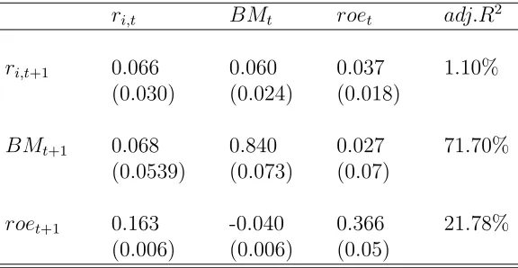
Table 4.6: Firm Level VAR estimates
This table shows the pooled-OLS parameter estimates for a first-order firm-level VAR
model. The model state vector includes the log stock return (r), log book-to-market
(BM), and log profitability (roe). All three variables are market adjusted, r by
sub-tracting CRSP value weighted returns and BM and roe by removing the respective year-specific cross-section mean. Standard errors (in parentheses) take into account clustering in each cross-section. The sample period for the dependent variables is 1965 to 2006, 58373 firm-years.
ri,t BMt roet adj.R2
ri,t+1 0.066 0.060 0.037 1.10%
(0.030) (0.024) (0.018)
BMt+1 0.068 0.840 0.027 71.70%
(0.0539) (0.073) (0.07)
roet+1 0.163 -0.040 0.366 21.78%
(0.006) (0.006) (0.05)
0.1M Et)/M Et), where BEt−1 is book equity for the fiscal year ending in calendar
year t-1, andM Et is the market equity at the end of May of year t. Log profitability
is also transformed and, hence, defined as log(1 +N It/(0.9BEt−1+ 0.1M Et)), where
N Itis the firm’s net income in year t. This firm-level VAR can be estimated through
pooled regressions.
Parameter estimates and errors generate market-adjusted cash flow and discount
rate news. Campbell et al. (2009) observe that one can use pooled regressions when
working with an unbalanced panel, where the average number of firms is much greater
than the number of annual observations. Conditioning on survival could bias
esti-mates. Therefore, it is assumed that the VAR transition matrix is equal for all firms.
in line with the literature. I make use of the coefficient matrix to recover firms’ cash
flow and discount rate news4
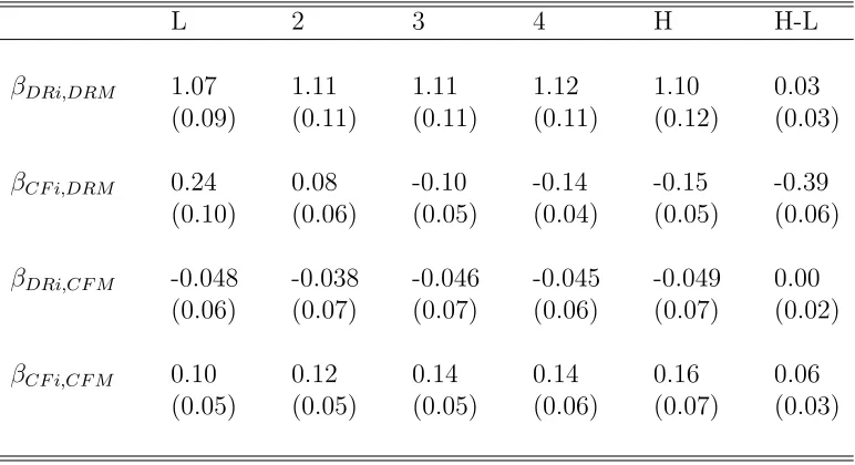
Table 4.7 show that the high (low) betas of low leverage stocks with the market
discount rate (cash-flow) shocks are determined by the properties of their cash flows.
That is, the cross-sectional differences in sensitivities among leverage portfolios are
determined by firms’ cash flow exposures to market innovations. The sensitivity of
discount rate innovations to market discount rate innovations is equally important
for all firms, and its magnitude is essentially the same for all portfolios.
These findings capture an important effect usually not examined in studies of
capital structure decisions. Generally, papers pay attention to the permanent impacts
on cash flows. Here, the short-run impact on cash flows seems to be relatively more
important for firms.
Indeed, the cash flow sensitivity to market cash flow news, what literature usually
calls cash flow risk, is monotonically increasing in leverage and its difference between
the two extreme portfolios is statistically significant. However, these betas are low
and not so economically different of each other. This sensitivity has been argued to
capture permanent effects on cash flows. On the other hand, what is striking is the
magnitude and high difference between the cash flow sensitivity to market discount
rate news. In fact, this beta for low leverage firms is 0.24 and for high leverage firms
is -0.15.
4The persistence of the VAR explanatory variables may cause bias in the estimates of
Table 4.7: Four Beta Decomposition
This table reports the firm-level news components of the discount-rate and cash flow betas measured for book leverage-sorted portfolios in Table II, panel A . They are
βCF i,CF M =
Cov(Ni,CFt+1,NM,CFt+1)
V ar(rM,t+1) , βCF i,DRM =
Cov(Ni,CFt+1,−NM,DRt+1)
V ar(rM,t+1) , βDRi,CF M =
Cov(−Ni,DRt+1,NM,CFt+1)
V ar(rM,t+1) , βDRi,DRM =
Cov(−Ni,DRt+1,−NM,DRt+1)
V ar(rM,t+1) . To construct portfolio
news terms, firm-level Ni,DR and Ni,CF are first extracted from the market-adjusted
firm-level panel VAR, then the corresponding market-wide news terms are added back, and finally the resulting firm-level news terms are value-weighted, as suggested by Campbell et al. (2009). The portfolio i=L is the extreme low leverage portfolio and i=H is the extreme high leverage portfolio. H-L represents the difference be-tween extreme high and low leverage portfolios. Standard errors are in parentheses, estimated using the Newey-West Method with five lags.
L 2 3 4 H H-L
βDRi,DRM 1.07 1.11 1.11 1.12 1.10 0.03
(0.09) (0.11) (0.11) (0.11) (0.12) (0.03)
βCF i,DRM 0.24 0.08 -0.10 -0.14 -0.15 -0.39
(0.10) (0.06) (0.05) (0.04) (0.05) (0.06)
βDRi,CF M -0.048 -0.038 -0.046 -0.045 -0.049 0.00
(0.06) (0.07) (0.07) (0.06) (0.07) (0.02)
βCF i,CF M 0.10 0.12 0.14 0.14 0.16 0.06
Since it is considered that firms manage their capital structures to maximize
share-holder wealth, it is possible that these sensitivities are related to the determinants
of leverage. That is, the results suggest that firms react to these risks to set their
capital structure. For example, a manager could consider financial flexibility as an
important factor influencing his decisions, and the degree of the impact of a short-run
shock in the firm’s cash flow can be fundamental to determine the correct level of
leverage in the balance sheet. In Chapter 5, I take a first step to understand this
claim by analyzing potential determinants of these betas.
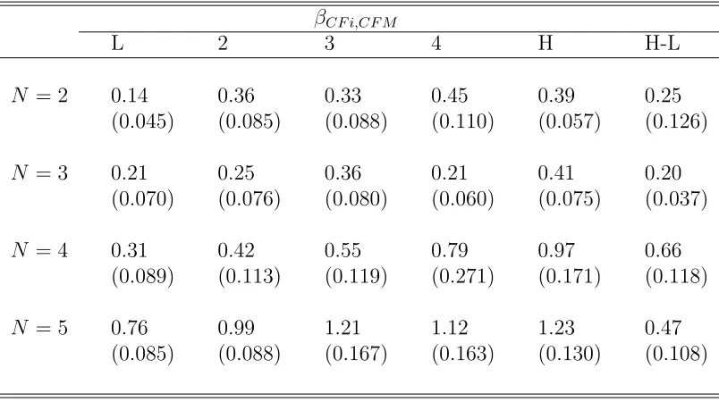
As shown in tables 4.8 and 4.9, both alternative implementations give the same
pattern in betas as obtained through the VAR approach. More important, the
long-run risk implementation, which is based on the cash-flow predictability, provides the
same patterns in cash-flow betas. The magnitudes are somewhat different, basically
due to both the choice of measures to proxy for cash flow and discount rate news and
the different horizons used. However, these findings confirm the effect of short and
long run shocks on firms’cash flow innovations, and reinforce the positive (negative)
relation between firms’cash flow innovations and market cash flow (discount rate)
Table 4.8: Long Run Risk Implementation
This table reports the firm-level news components of the discount-rate and cash flow betas measured for book leverage-sorted portfolios. The sensitivities of portfolios’ cash flow innovation to market cash flow news is given by the slope of the following regression:
N X
j=1
ρjgi,t+j,j+1 =α+βCF i,CF M N X
j=1
ρjgM,t+j,j+1+
The portfolio i=L is the extreme low leverage portfolio and i=H is the extreme high leverage portfolio. H-L represents the difference between extreme high and low lever-age portfolios. Standard errors (in parentheses) are estimated using the Newey-West Method with five lags.
βCF i,CF M
L 2 3 4 H H-L
N = 2 0.14 0.36 0.33 0.45 0.39 0.25
(0.045) (0.085) (0.088) (0.110) (0.057) (0.126)
N = 3 0.21 0.25 0.36 0.21 0.41 0.20
(0.070) (0.076) (0.080) (0.060) (0.075) (0.037)
N = 4 0.31 0.42 0.55 0.79 0.97 0.66
(0.089) (0.113) (0.119) (0.271) (0.171) (0.118)
N = 5 0.76 0.99 1.21 1.12 1.23 0.47
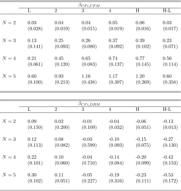
Table 4.9: Direct Proxies Implementation
This table reports the firm-level news components of the discount-rate and cash flow betas measured for book leverage-sorted portfolios. Portfolio level cash-flow news are the following:
Ni,CF,t+1= N
X
j=1
ρj−1roei,t,t+j
whereroei,t,t+j is the log of real profitability for portfolio i, sorted in year t, and measured in year t+j. Discount-rate news at the market level are:
−NM,DR,t+1= N
X
j=1
[ρj−1∆t+jln(P/E)M]
The portfolio i=L is the extreme low leverage portfolio and i=H is the extreme high leverage portfolio. H-L represents the difference between extreme high and low leverage portfolios. Standard errors (in parentheses) are estimated using the Newey-West Method with five lags.
βCF i,CF M
L 2 3 4 H H-L
N = 2 0.03 0.04 0.04 0.05 0.06 0.03 (0.028) (0.019) (0.015) (0.019) (0.016) (0.017)
N = 3 0.13 0.25 0.26 0.37 0.39 0.23 (0.141) (0.093) (0.080) (0.092) (0.102) (0.071)
N = 4 0.21 0.45 0.65 0.74 0.77 0.56 (0.061) (0.120) (0.083) (0.137) (0.145) (0.114)
N = 5 0.60 0.93 1.16 1.17 1.20 0.60 (0.100) (0.213) (0.438) (0.397) (0.269) (0.358)
βCF i,DRM
L 2 3 4 H H-L
N = 2 0.09 0.02 -0.01 -0.04 -0.06 -0.13
(0.150) (0.200) (0.109) (0.032) (0.051) (0.013)
N = 3 0.12 0.08 -0.03 -0.10 -0.15 -0.27
(0.113) (0.082) (0.599) (0.093) (0.075) (0.130)
N = 4 0.22 0.10 -0.04 -0.14 -0.20 -0.42
(0.101) (0.060) (0.710) (0.084) (0.099) (0.153)
N = 5 0.30 0.11 -0.05 -0.19 -0.23 -0.53
Chapter 5
Determinants of Risk Exposures
and Capital Structure
We noted there is a relevant heterogeneity in betas between firms’ capital structures,
which seems to be related to temporary and permanent systematic shocks affecting
firms’ cash flows. Moreover, the importance of these shocks is different for firms with
different book leverages. The next step is to investigate what determines these betas.
Since financial leverage seems to be an output of an optimal decision, it is natural to
associate these betas with variables used to explain the cross sectional heterogeneity
of firms’ capital structures.
In a related study, Gorbenko and Strebulaev (2009) also argue that temporary
and permanent idiosyncratic shocks to firms’ cash-flows have different impacts on
corporate financial policies. They build a theoretical model with potential predictions
in line with the empirical observations about financial conservatism and low leverage
phenomena.
Frank and Goyal (2007b) examine an extensive list of factors which could
con-ceivably explain why heterogeneity exists between firms’ capital structures. They
conclude that only profitability, firm size, market-to-book, median industry leverage,
coefficients are statistically significant in a predictive regression, where the dependent
variable is leverage. However, they together only explain about 25% of the total
vari-ation. What is interesting is that accounting measures of risk, market conditions and
macroeconomic variables are not significant.
Indeed, what is generally considered in capital structure theory is the volatility
(idiosyncratic) risk of cash flows. Trade-off theory argues that firms with more volatile
cash flows face higher expected costs of financial distress and should use less debt.
More volatile cash flows reduce the probability that tax shields will be fully utilized.
Thus higher risk should result in less debt. Pecking order theory predicts that firms
with volatile stocks suffer more from adverse selection. Hence ”riskier” firms have
higher leverage.
Here, I depart from this view and analyze how systematic risk is associated with
capital structure decisions by investigating the relation between variables successfully
used as leverage predictors and cash-flow betas.
I use a parsimonious list of factors considered to have some influence on corporate
leverage, analyzing some of the variables proposed by Frank and Goyal (2007b) and
including capital expenditures as an alternative proxy for growth, and probability
of default to be extensively used as a direct proxy related to financial distress risk.
Then, the final set of variables is composed of profitability (ROA), unlevered z-score,
tangibility, capital expenditures (capex), firm size, and book-to-market.
Although this choice relies fundamentally on the implications of the main theories
of capital structure decisions, I do not specifically test a particular theory. Instead
of predicting leverage directly, I investigate whether book leverage is associated with
two sources of cash-flow risks, and use cross-sectional firm-level regressions to identify
given by extant theories seem uncontroversial, there is significant disagreement in
some cases. For example, trade-off theory predicts that profitable firms use more
debt given their lower expected costs of financial distress. In a dynamic tradeoff
model, leverage appears to be negatively related to profitability. For the pecking
order theory more profitable firms will become less leveraged over time.
Therefore, I consider the effects both on the entire sample and on the two extreme
low and high leverage portfolios to capture any asymmetric effect of these variables
on risk sensitivities. This investigation has two purposes. First, it allows studying the
effect of well documented leverage predictors on betas. Second, it helps in inferring
the existence of any unobserved factor related to leverage not captured by the existing
predictors.
Although the subject of this study is not to make an extensive analysis of the
determinants of leverage, the fact that leverage is clearly associated with betas seems
to be informative about capital structure decisions. If the variables expected to
explain it are not completely related to these betas, and betas have a clear relation
to financial leverage, we can argue that there is something missing. In fact, Lemmon,
Roberts, and Zender (2008) acknowledge the importance of an unobserved factor
(firm fixed effect) which explains much of the heterogeneity in leverage.
I check how these factors responds to market shocks. Specifically, I estimate the
following equations1:
(Ni,CF,t)×(NCF M,t) =Xi,t−1B +ui,t (5.1)
(Ni,CF,t)×(−NDRM,t) =Xi,t−1B +ui,t (5.2)
1Campbell et al. (2009) explore a similar regression and relate the characteristics of each stock
Equations (5.1) and (5.2) link the components of firms’ risks to predictors of each
firm’s leverage. The estimation technique is as follows. First, I cross-sectionally
de-mean both firms’ cash flow innovations and independent variables. Next, I normalize
the independent variables to have an unit variance. After estimating the regressions,
I divide the coefficients by market variance. The results presented in Table 5.1
rep-resent the effect on betas of a one-standard deviation change in the independent
variable.
The first two columns in table 5.1 show that all variables, but book-to-market,
predict cash-flow cash-flow beta, and all variables, but capital expenditures and log
assets, predict cash-flow discount-rate beta. That is, variations in book-to-market are
solely associated with short-term sensitivities of cash flows and variations in capital
expenditures and firms’ assets are solely associated with long-term sensitivities of
cash flows.
Some aspects stand out in this table. Positive changes in firm’s profitability
decreases its cash flow sensitivity to market cash flow news (permanent), but increases
significantly its sensitivity to market discount rate news (transitory). As cash flows
becomes larger, the importance of temporary shocks will be much higher, even though
permanent shocks have either little or zero effect on cash flows.
Specifically, as firms become more profitable, permanent shocks to their cash flows
are attenuated. Actually, the sensitivity of cash flow innovations to market cash flow
news is low, but negative. It seems to indicate that more profits signal good future
prospects, and that these firms become more diversified. A similar interpretation
could be applied when we look at firm size (log assets). For both extreme portfolios,
larger firms are less sensitive to permanent shocks only.