Fluid-Structure Interaction models in pressurized
fluid-filled pipes: a review
David Ferr`as1, Pedro A. Manso2, Anton J. Schleiss2, and D´ıdia I.C. Covas3
1Department of Environmental Engineering and Water Technology, IHE Delft
Institute for Water Education (The Netherlands)
2Laboratory of Hydraulic Constructions (LCH), ´Ecole Polytechnique F´ed´erale de
Lausanne (Switzerland)
3CERIS, Instituto Superior T´ecnico, Universidade de Lisboa (Portugal)
Abstract
The present review paper aims at collecting and discussing the re-search work, numerical and experimental, carried out in the field of Fluid-Structure Interaction (FSI) in one-dimensional (1D) pres-surized transient flow in the time-domain approach. Background theory and basic definitions are provided for the proper understand-ing of the assessed literature. A novel frame of reference is pro-posed for the classification of FSI models based on pipe degrees-of-freedom. Numerical research is organized according to this classifi-cation, while an extensive review on experimental research is pre-sented by institution. Engineering applications of FSI models are described and historical accidents and post-accident analyses docu-mented.
Keywords: hydraulic transients, water-hammer, fluid-structure interaction, degrees-of-freedom, junction coupling, Poisson coupling, friction coupling, Bourdon coupling.
1
Notation
Af fluid cross-sectional area (m2) p fluid pressure (Pa)
af pressure wave speed (ms−1) r radius of the pipe-wall (m) Ap pipe-wall cross-sectional area (m2) R rotational velocity (rad s−1) an acoustic speed of thei-DOF (ms−1) Rc bend radius of curvature (m)
D pipe inner diameter (m) t time (s)
E pipe-wall Young’s modulus (Pa) U pipe-wall velocity (ms−1) e pipe-wall thickness (m) V fluid mean velocity (ms−1) G shear modulus (Pa) W pipe-wall radial velocity (ms−1) I second moment of area (m4) ν Poisson’s ratio (–)
J polar second moment of area (m4) ρf fluid density (kgm−3) K bulk modulus of compressibility (Pa) ρp pipe density (kgm−3)
L pipe length (m) σ pipe-wall stress (Pa)
M moment (N m) strain (–)
1
1
Introduction
2
The first scientific contributions to the field of Fluid-Structure Interaction (FSI) in
tran-3
sient pipe flow took place in the 19th century when authors like Korteweg (1878) or
4
Helmholtz (1882) realized about the need of considering both fluid compressibility and
5
pipe-wall distensibility as interacting mechanisms. Classical water-hammer theory is also
6
based on this principle. Since then, many researchers have added their contributions in a
7
step-wise manner, building up and shaping the theory of hydraulic transients in pipe flow.
8
FSI models deal with the original principle of considering water-hammer waves as a
9
result of the relation between fluid and pipe deformations. Skalak (1955) presented a
10
milestone PhD thesis entitled‘An extension of the theory of water-hammer’. The basis of
11
one-dimensional (1D) FSI was established, pipe vibration modes were described and the
12
basic formulation for straight pipes was presented. Skalak’s work triggered the FSI research
13
on the two-way coupling between fluid dynamics and structural mechanics. Contributions
14
by Wilkinson (1977), Walker & Phillips (1977), Valentin et al. (1979), Wiggert et al.
15
(1985a), Wiggert(1986), Joung & Shin (1987), B¨urmann & Thielen(1988a), Wiggert &
16
Tijsseling (2001) and Tijsseling (2003) developed and completed the theory for all the
17
basic degrees-of-freedom (DOF) of pipe-systems.
18
Some historical reviews on hydraulic transients in pipe flow are given byWood(1970),
19
Thorley (1976), Anderson (1976), Tijsseling & Anderson (2007), Tijsseling & Anderson
20
(2008) and Tijsseling & Anderson (2012). The developments in water-hammer research
21
before the 20th century are well summarized by Boulanger(1913). AlsoLambossy (1950)
22
and Stecki & Davis(1986) presented in-depth reviews that served, at that time, as vision
23
papers. More recently,Ghidaouiet al.(2005) presented a complete state-of-the-art review
24
focusing on both historic and most recent research and practice covering most of the
water-25
hammer research topics. Surveys more specific in the field of Fluid-Structure Interaction
are given by Wiggert (1986), Tijsseling (1996), Wiggert & Tijsseling (2001) and, more
27
recently, byLiet al.(2015). The aim of the current review is to report the most significant
28
contributions carried out in water-hammer research related to Fluid-Structure Interaction
29
in 1D hydraulic transients modelling, giving emphasis on the time-domain analyses and
30
focusing on the most recent research. A novel classification of FSI models based on
pipe-31
degrees-of-freedom is presented.
32
The paper starts with the basic definitions and background theory that frame the
33
research of FSI in water-hammer modelling. Numerical and experimental research is
doc-34
umented following the physically-based classification of pipe degrees-of-freedom. Finally,
35
insights of engineering applications of Fluid-Structure Interaction developments in pipe
36
flow are pointed out.
37
2
Definitions and basic concepts
38
2.1
Fluid-Structure Interaction
39
In the present review, Fluid-Structure Interaction in pipe systems is defined as the transfer
40
of momentum and forces in both ways, between the pipe-wall and the contained fluid
41
during unsteady flow (Wiggert,1986). Hence, FSI in pipe flow involves, at least, transient
42
responses of two different physical systems. The interaction arises when the time scales of
43
both system responses are shorter than the time scale of the overall transient event (i.e.
44
time lag between the initial and the final steady state). If the disturbance source is shorter
45
than both system responses, then fast fluid and solid transients simultaneously occur. If
46
their interaction is strong enough, then the description of FSI might be worthwhile in
47
water-hammer analyses and interaction mechanisms have to be taken into account.
48
In a broad sense, Fluid-Structure Interaction embraces any form of energy transfer,
49
one upon another, between the fluid and the structure. In common engineering problems,
50
this transferred energy is typically kinetic and elastic or thermal. The former is termed
51
mechanical Fluid-Structure Interaction and the latter thermal Fluid-Structure Interaction.
52
Heat exchange effects in transient pipe flow are barely significant, processes are assumed
53
adiabatic, and FSI analyses are mainly focused on the momentum exchange between the
54
fluid and the pipe structure.
55
Two different approaches may be followed to account for the momentum transfer into
56
the structure (Giannopapa,2004): considering that the structure moves as a rigid solid or
57
by the propagation of a local excitation/deformation of the solid. In the first, no transient
58
event is considered propagating throughout the solid, the structure element moves as a
59
rigid body and its effect on the fluid is analysed. In the second, the modes of vibration
60
of the structure element are excited and their respective transient states are taken into
61
account and coupled with the fluid transient. The present review is focused only on the
62
second form.
63
FSI analyses may be classified according to the dimensions and the degrees-of-freedom
64
with which the pipe system is allowed to move. Normally, in 1D water-hammer analysis,
65
the classification criterion is based on the modes of vibration of the pipe, which is quite
convenient for frequency-domain approaches. However, for time-domain analyses a
clas-67
sification based on the pipe degrees-of-freedom is more physically intuitive. The latter is
68
the classification criterion used herein.
69
2.2
Degrees-of-freedom in fluid-filled pipes
70
Degrees-of-freedom (DOF) are the number of independent coordinates or parameters that
71
describe the position or configuration of a mechanical system at any time (Sinha,2010).
72
Systems with finite number of degrees-of-freedom are called discrete systems, and those
73
with infinite degrees-of-freedom are called continuous systems. Pipe systems are
contin-74
uous systems, however these can be treated as discrete systems for numerical modelling
75
purposes, with many DOF’s depending on the number of nodes.
76
Pipes are slender elements, therefore a 1D approach assuming that the fluid pressure
77
propagates axially during hydraulic transients is reasonable. However, transient pressures
78
transmit forces over the pipe wall that make the pipe system move in a 3D space. The
79
basic degrees-of-freedom for a rigid body in a 3D space are three for translation (i.e.
80
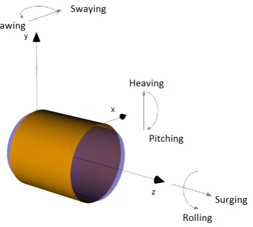
heaving, swaying and surging) and three for rotation (i.e. pitching, yawing and rolling).
81
An infinitesimal control volume of a pipe-segment (like in Fig. 1) will have the referred
82
six basic degrees-of-freedom. The pipe-wall control-volume is a hollow cylinder, therefore
83
axisymmetric vibration due to hoop strain must be as well considered, adding another
84
degree-of-freedom. Additionally, the infinitesimal control volume of the 1D contained
85
fluid accounts for another degree-of-freedom. Henceforth, in the present 1D FSI analysis,
86
eight degrees-of-freedom compose the infinitesimal control volume of a pipe.
87
For each degree-of-freedom, momentum and mass conservation laws are applied, giving
88
as result a set of 16 partial differential equations (cf. Eqs. 1 to16), with time and space
89
coordinates as independent variables, governing two basic dependent variables related
90
with the loading and the movement in each degree-of-freedom (i.e., load and deformation
91
relation). Depending on the pipe geometry, axial, shear, bending and torsional forces and
92
displacements alternate throughout the pipe. A schematic of such displacements is shown
93
in Fig. 1.
Fig. 1: Spatial reference system and signs convention in a straight pipe element
FSI models in 1D water-hammer analyses can be classified according to the pipe
95
degrees-of-freedom as follows:
96
• 1-DOF (fluid surging): only the axial fluid transient event is described.
97
• 2-DOF (breathing): radial inertia of the fluid and the pipe are taken into account.
98
• 3-DOF (solid surging): refers to the axial movement of the pipe.
99
• 4-DOF (swaying): includes the effect of horizontal displacement of the pipe.
100
• 5-DOF (heaving): includes the effect of vertical displacement of the pipe.
101
• 6-DOF (yawing): includes the rotation of the pipe in the xzc plane.
102
• 7-DOF (pitching): includes the rotation of the pipe in thecyz plane. 103
• 8-DOF (rolling): includes the rotation of the pipe on the cxy plane. 104
2.3
Fundamental formulae
105
The equations of the system (Eqs. 1 to 16) presented hereby correspond to the basic
106
momentum and continuity conservation equations of a pipe-system with eight
degrees-of-107
freedom, like in the control volume depicted in Fig. 1. Thin-wall assumption is adopted.
108
Eqs.1 to6 and their associate characteristic equations can be found inWalker & Phillips
109
(1977); Eqs. 7 to16inWiggert et al. (1987). The symbols are declared in the Notation.
1-DOF (fluid surging): ∂V
∂t + 1 ρf
∂p
∂z = 0 (1)
1 K
∂p ∂t +
∂V ∂z =−
2
rW (2)
2-DOF (breathing):
ρpre+ρfr 2
2
∂W
∂t =rp−e σθ (3)
∂σθ ∂t −Eν
∂Uz ∂z =E
W
r (4)
3-DOF (solid surging): ∂Uz
∂t − 1 ρp
∂σz
∂z = 0 (5)
1 E
∂σz ∂t −
∂Uz ∂z =ν
W
r (6)
4-DOF (swaying):
−
ρp+ Af Apρf
∂Ux ∂t +
∂σx
∂z = 0 (7)
∂σx ∂t −G
∂Ux
∂z =−GRy (8)
5-DOF (heaving):
−
ρp+Af Ap
ρf
∂Uy ∂t +
∂σy
∂z = 0 (9)
∂σy ∂t −G
∂Uy
6-DOF (yawing):
−ρpIp ∂Ry
∂t + ∂My
∂z =−σxAp (11)
∂My ∂t −EIp
∂Ry
∂z = 0 (12)
7-DOF (pitching):
−ρpIp∂Rx ∂t +
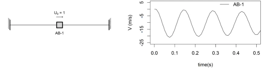
∂Mx
∂z =σyAp (13)
∂Mx ∂t −EIp
∂Rx
∂z = 0 (14)
8-DOF (rolling):
−ρpJ ∂Rz
∂t + ∂Mz
∂z = 0 (15)
∂Mz
∂t −GJ
∂Rz
∂z = 0 (16)
All the degrees-of-freedom are distinguished in the previous system of equations, hence
111
the analysis of wave celerities can be reduced to the essential (uncoupled) wave propagating
112
speeds in each degree-of-freedom. The following formulae (Eqs. 17 to 21) define the
113
uncoupled wave celerities for each wave type considered (note that the sub-index refers to
114
the DOF):
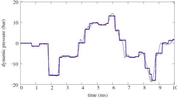
115
a1=
s
K ρf
(17)
116
a3 =
s
E
ρp (18)
117
a4,5 =
s
GAp
ρpAp+ρfAf (19)
118
a6,7 =
s
EIp ρpIp+ρfIf
(20)
119
a8 =
s
G ρp
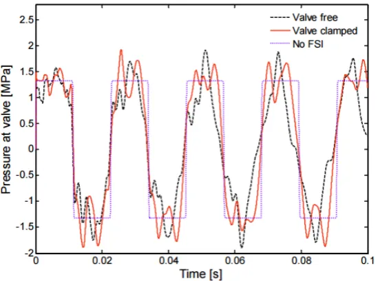
(21)
Notice that, due to the pipe axisymmetry, shear and bending wave celerities are equal
120
in both planes (i.e. a4 =a5 and a6=a7). Due to the dispersive nature of a 2-DOF wave
propagating along the pipe-wall, no formula for a2 is provided (Tijsseling & Anderson,
122
2012).
123
The advantage of considering the system of Eqs. 1 to 16 is that there is no need of
124
considering the abstract concept of elastic wave celerity from classic water-hammer theory.
125
An in-depth critical analysis of the different interpretations of wave speed in both time
126
and frequency-domains is given by Tijsseling & Vardy(2015).
127
2.4
Coupling mechanisms and modelling approaches
128
Pipe systems subjected to water-hammer transients can be regarded as
free-damped-129
deterministic vibrating systems with multiple modes of vibration, coupled or uncoupled,
130
according to the degrees-of-freedom of the conduit and exposed to skin friction, dry friction
131
and structural/hysteretic damping. Although not included in Eqs. 1to16, these damping
132
mechanisms convert hydraulic transients into non-periodic and non-linear phenomena that
133
are difficult to analyse.
134
The different degrees-of-freedom of a pipe system may interact one upon another.
135
There are three basic kinds of coupling mechanisms (Tijsseling,1996): (i)Poisson coupling
136
describes the interaction between the axial motion of the pipe-wall and the pressure in
137
the fluid occurring by means of the Poisson effect; (ii) friction coupling arises from the
138
shear stress between the pipe-wall and the fluid; (iii) and junction coupling results from
139
unbalanced local forces and by changes in the fluid momentum that occur in pipe bends,
140
T-junctions or cross-section changes.
141
In time-domain analyses, the Method of Characteristics (MOC), the Finite Element
142
Method (FEM), the Finite Difference Method (FDM) or the Finite Volume Method (FVM)
143
are discretization methods used to solve the governing differential equations. Either a
144
single or combined (hybrid) numerical method can be used for the description of the
145
different degrees-of-freedom of the pipe. The method of characteristics (MOC) and the
146
finite-element method (FEM), or a combination of both, are the most common numerical
147
methods used for solving the one-dimensional basic equations (Tijsseling, 1996). One
148
single integrating approach, such as MOC-MOC or FEM-FEM, is convenient as all the
149
information flows into the same numerical scheme (Wiggert & Tijsseling, 2001). Other
150
combinations are not that common in one-dimensional analyses; FVM is rather used for
151
3D simulations.
152
A different coupling approach consists of setting up an interaction between two different
153
computer codes, one specific for the fluid and another for the structure. In each time-step
154
output information is transferred in both directions. There are contributions proposing
155
methodologies to carry out this data transfer, such asWare & Williamson(1982). However,
156
the main challenge of this approach is the requirement of a considerable computational
157
effort and data transfer (Belytschkoet al.,1986).
158
A-Moneim & Chang(1978) coupled FDM code for the fluid and a FEM for the
struc-159
ture with the goal to simulate an interesting experimental research carried out at the
Stan-160
ford Research Institute (SRI). Other authors who tried to simulate the same validating
161
experiments are Romanderet al. (1980) and Kulak(1982,1985) who coupled FEM-FEM
software. Also Erath et al. (1998, 1999) used a FDM code for the fluid with a FEM for
163
the structure with the goal to simulate field measurements from a pump shut-down and a
164
closing valve in the nuclear power plant KRB II (Gundremmingen, Germany). Bietenbeck
165
et al. (1985) andMueller (1987) applied a MOC-FEM coupling aiming at describing the
166
response of an experimental facility located at the Karlsruhe Nuclear Research Centre
167
(KfK–Kernforschungszentrum Karlsruhe).
168
InCasadeiet al.(2001) FEM and FVM are compared for the fluid domain simulation
169
and coupling techniques are proposed. In Sim˜ao et al. (2015a,b) the traditional MOC
170
approach for the fluid is compared with a CFD k−model, coupled with a FEM model
171
for the structure.
172
3
Numerical and experimental research
173
3.1
Introduction
174
A review of the numerical and experimental research of 1D FSI in the time-domain is
175
presented hereby. Table 1 summarizes and describes the main FSI models according to
176
their DOF’s and lists some of the most relevant contributions that enabled the
theoret-177
ical development, implementation, application and validation of numerical models using
178
adapted versions of the fundamental equations presented in subsection 2.3. Details of
179
these research contributions are provided in the following subsections.
Tab. 1: Summary table of main 1D FSI models in hydraulic transients research.
DOF Description Main contributions
1 Only the fluid transient is described. Equations solved: 1,2
Menabrea(1858);Korteweg(1878);
Von Kries(1883);Frizell(1898);
Allievi(1902);Joukowsky(1904);
Halliwell(1963)
1,3 Solid surging is coupled with the fluid. Equations solved: 1,2,5, 6
Schwarz(1978);Wiggert(1983);
Kojima & Shinada(1988);
B¨urmann & Thielen (1988c);
Lavooij & Tijsseling(1991);
Zhanget al. (1994);Vardy et al.(1996);
Liet al.(2003);Tijsseling(2003);
Gale & Tiselj(2005);
Loh & Tijsseling(2014);
Ferraset al.(2017b)
1,2,3
Fluid, breathing and solid surging interact. Equations solved:
1,2,3,4,5, 6
Walker & Phillips(1977);
Schwarz(1978);
Kellneret al.(1983);
Gormanet al.(2000);
Tijsseling(2007)
1,3 and 4,6 or 5,7
Fluid and solid surging, and either swaying and yawing or heaving and pitching are taken into account. Equations solved: 1,2,5, 6
and7,8,11,12or9,10,13,14
Regetz(1960);
Wood & Chao(1971);
A-Moneim & Chang(1979);
Hu & Phillips(1981);
Tijsselinget al.(1994,1996);
Vardyet al.(1996);
Tijsseling & Heinsbroek(1999);
Gale & Tiselj(2006);
Sim˜aoet al.(2015b)
1,3,4,5,6,7,8
Fluid and solid surging, swaying, heaving, yawing, pitching and rolling are coupled. Equations solved:
1,2,5,6,7, 8,9,10,11,12,
13,14,15,16
Weijde(1985);
Tijsseling & Lavooij(1990);
Lavooij & Tijsseling(1989,1991);
Kruisbrink(1990);
Bettinaliet al.(1991);
Heinsbroek(1997)
3.2
One degree-of-freedom models
181
The classic water-hammer model (two-equation model) is a sophisticated version of the
182
basic 1-DOF system (Eqs. 1 and 2), where the right-hand-side term of the continuity
183
equation is adapted in order to account for the pipe-wall distensibility. Although the
184
bulk modulus of compressibility and a finite acoustic wave speed are considered in the
185
fluid, in terms of density variation the fluid is assumed to be incompressible and pressure
186
changes are related to velocity changes by embedding fluid compressibility and pipe-wall
187
distensibility into the wave celerity value, which is regarded as a constant parameter and
188
can be either experimentally or numerically determined. Research works such as Young
(1808), Weber (1866), Resal (1876), Moens (1878), Korteweg (1878), Von Kries (1883)
190
or Halliwell(1963) contributed to the development of wave celerity formulae. The latest
191
presented correcting factors to account for axial FSI.
192
The fundamental equations of classic water-hammer theory (i.e. mass and momentum
193
conservation) can be derived from Navier-Stokes equations (Ghidaoui,2004) or by directly
194
applying the Reynolds Transport Theorem (Chaudhry,2014) to a control volume of the
195
pipe. From an FSI standpoint, these fundamental equations can be also reached from the
196
system of equations presented in Section2, as the classical theory considers a combination
197
of the first two degrees-of-freedom. The fundamental momentum conservation equation is
198
directly the one presented in 1-DOF (Eq.1). For mass conservation (continuity equation),
199
the cross-sectional area of the control volume is assumed to vary and this variation is
200
related to the fluid inner pressure by applying a quasi-static assumption in the 2-DOF.
201
This derivation is described in AppendixB.
202
The system of PDE’s (Eq. 22 and Eq. 23) represents the fundamental conservation
203
equations of classic frictionless water-hammer theory.
204
∂V ∂t +
1 ρf
∂p
∂z = 0 (22)
205
∂V ∂z +
1 ρfah
∂p
∂t = 0 (23)
Usually the system of mass conservation and momentum equations is solved by means
206
of the Method of Characteristics (MOC), which is the most popular and extensively used
207
method by researchers and engineers thanks to its easy programming, computational
ef-208
ficiency and accuracy of the results (Vardy & Tijsseling, 2015). Over all methods MOC
209
stays the closest to the physics of the problem.
210
3.3
Two degree-of-freedom models
211
The historical development of four-equation models can be traced back from Korteweg
212
(1878) who already pointed out the need of considering axial stress waves. Gromeka
213
(1883) and Lamb (1898), qualitatively, took into account pipe axial inertia and Poisson
214
coupling in their analyses. Skalak(1955), who extended Lamb’s work, presented the four
215
basic fundamental equations and introduced the concept of precursor waves. Thorley
216
(1969) was the first to experimentally observe precursor waves, which are, at the same
217
time, the evidence of the Poisson coupling effect. B¨urmann(1979),Thielen & B¨urmann
218
(1980) and B¨urmann & Thielen(1988b) used the simplified version of Skalak’s equations
219
which represent the well-known four-equation system for axial FSI. Skalak’s work was
220
revisited and analysed in Tijsselinget al. (2008).
221
For the description of pressure waves in pipe systems, two or four-equation models
222
are sufficient (Tijsseling,1996). Four-equation models consider the combination of classic
223
theory with the 3-DOF equations. Hence, four fundamental equations, two for the fluid
224
and two for the pipe axial movement, are to be solved. The right-hand-side terms of
225
the continuity equations of the 1-DOF and 3-DOF systems must be adapted in order to
describe the Poisson coupling in terms of the dependent variables of the four-equation
227
model (i.e., respectively, axial stress of the pipe-wall and fluid pressure). This derivation
228
is explained in Appendix Cfrom which Eqs. 25 and 27are obtained.
229 ∂V ∂t + 1 ρf ∂p
∂z = 0 (24)
230
∂V ∂z +
1 ρfa2h
∂p ∂t = 2ν E ∂σz ∂t (25) 231 ∂Uz ∂t − 1 ρp ∂σz
∂z = 0 (26)
232
∂Uz ∂z −
1 ρpa23
∂σz ∂t =−
rν eE ∂p ∂t (27) E 233
Several numerical methods can be used to solve the above system of equations, either
234
integrating both the fluid and the structure in the same numerical scheme (e.g.,
MOC-235
MOC) or by a combination between different schemes (e.g.,MOC-FEM).
236
In B¨urmann (1979) and B¨urmann & Thielen (1988b) the four-equation system was
237
solved using MOC procedure for the first time. B¨urmann(1975,1979) and B¨urmann &
238
Thielen (1988c) presented a series of tests carried out on a vertical pipe line located in
239
a subterranean salt cavern. In B¨urmann et al. (1985, 1986b, 1987) measurements were
240
shown from a water-main bridge, and inB¨urmannet al.(1986a) andB¨urmann & Thielen
241
(1988a) from a loading line between tanks and ships. These measurements were used to
242
develop and validate the four-equation model and to understand FSI mechanisms.
243
In Vardy & Alsarraj (1989) the Method of Characteristics for both the fluid and
244
the structure (i.e., MOC-MOC) was shown to have useful advantages. This approach
245
was supported by experimental evidence from Vardy & Fan (1986,1987,1989) andFan
246
(1989), who carried out measurements in which FSI effects were particularly well isolated
247
by means of suspended pipe rigs that were excited by the impact of a solid rod. In
248
combination with their numerical developments, they showed how FSI coupling changes
249
the natural vibrating frequencies, which cannot be predicted by uncoupled approaches.
250
Schwarz(1978) used a FDM scheme in his four-equation model as a simplified version
251
of a six-equation model which was solved by MOC. Ellis (1980) modelled fluid and axial
252
stress waves in conduits by means of MOC, taking into account only junction coupling
253
(ignoring Poisson coupling). Kojima & Shinada(1988) also used a FDM approach which
254
was validated by tests on a thin-walled straight pipe for Poisson coupling as well as junction
255
coupling at a closed-free pipe end. Ferr`aset al.(2016a) derived an explicit Joukowsky-like
256
expression from the four-equation system aiming at estimating maximum pressures during
257
water-hammer with FSI.
258
Wiggertet al.(1985a),Elansary & Contractor(1990,1994),Elansaryet al.(1994) and
259
Budny et al.(1991) explained how to solve the four-equation system considering Poisson
260
coupling. They presented the characteristic equations after MOC transformation and how
261
to integrate them within the same characteristic grid using time-line interpolations as
explained by Goldberg (1983). The MOC transformation that allows hyperbolic partial
263
differential equation systems to be converted to a set of ordinary differential equations
264
was based on Forsytheet al.(1960). Zhanget al.(1994) used a FEM scheme for both the
265
fluid and the structure. InBouabdallah & Massouh(1997) andGhodhbani & Hadj-Ta¨ıeb
266
(2013), time interpolation and wave adjustment methods are compared for MOC-MOC
267
solutions. Wiggert (1983) used a hybrid MOC-FEM approach, MOC for the fluid and
268
FEM for the structure, and experimental data was used for model verification. A FVM
269
approach was presented in Gale & Tiselj (2005) to solve the four-equation model, which
270
was successfully verified using the Delft Hydraulics Benchmark Problem A (Tijsseling &
271
Lavooij,1990;Lavooij & Tijsseling,1991). InLavooij & Tijsseling(1991) both approaches
272
MOC-MOC and MOC-FEM are compared, concluding that for straight pipe problems the
273
MOC procedure is more accurate and efficient. Ferras et al. (2017a) used MOC-MOC
274
coupling to simulate a kind of FSI which was experimentally observed in pipe coils by
275
Ferr`aset al. (2014,2016a).
276
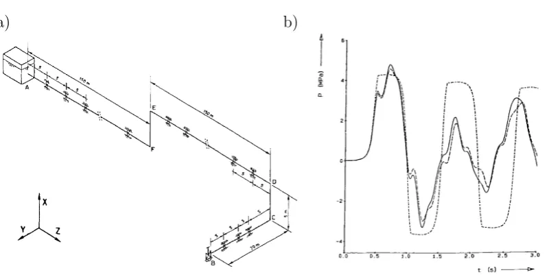
The Delft Hydraulics Benchmark Problem A (20 m long, steel pipe, 0.4 m diameter)
277
is a good test case for the verification of four-equation numerical codes (v.i. Fig.2). InLi
278
et al.(2003),Tijsseling(2003) andTijsseling(2009), a theoretical development of an exact
279
solution of the four-equation system by means of a recursion was presented. The drawback
280
of the method is its exponential computational effort for longer simulation periods.
Re-281
cently, in Loh & Tijsseling (2014), the computation for the exact solution was upgraded
282
in order to increase computational efficiency and applicability. The analysis suggested
283
to keep the scope of exact solutions to generate test cases and to benchmark solutions
284
for more conventional numerical methods. Also, in Xu & Jiao (2017), the efficiency is
285
improved by using a hybrid cubic time-line interpolation scheme.
286
It is important to highlight that numerical outputs, such as the one presented inv.i.
287
Fig.2, show how FSI phenomena can cause pressure surges higher than the ones expected
288
from classical theory. Tijsseling(1997) has demonstrated the Poisson coupling beat, which
289
is a phenomenon that arises from resonance between 1-DOF and 3-DOF. Poisson coupling
290
beat was already numerically observed byWiggert(1986). So far, there is no experimental
291
evidence about it, as damping mechanisms tend to hide the oscillating resonance between
292
the pipe-wall and the fluid vibrations.
293
More recently,Ferraset al.(2017b) numerically observed the Liebau effect in pipe flow
294
using a four-equation model which was adapted to describe the inertia of thrust blocks.
295
The Liebau effect is rather an object of study in the field of physiological flows and is
296
defined as the occurrence of valveless pumping through the application of a periodic force
297
at a place which lies asymmetric with respect to the system configuration (Borzi & Propst,
298
2003). Ferras et al. (2017b) claimed that the Liebau effect in pipe flow may be induced
299
by Poisson coupling and should be object of further research (v.i. Fig. 3).
Fig. 2: Four-equation code verified by means of the Delft Hydraulics Benchmark Problem A (Ferr`as,2016).
Fig. 3: Numerical evidence of Liebau effect depicted in Ferras et al.(2017b).
3.4
Three degree-of-freedom models
301
Six-equation models aim at describing the 1,2,3-DOF’s. As in the four-equation model,
302
similar numerical schemes can be used for solving the six-equation system. However, the
303
right-hand-sides of the three continuity equations are not expressed in differential terms.
304
A first or second-order approximation can be applied for integrating these equations.
305
Walker & Phillips(1977) were the first proposing and solving by MOC the six-equation
306
model. These authors have compared results from the frequency and time domains and
307
carried out their validation using experimental data collected from a water-filled copper
308
pipe excited by hammering the pipe-end.
With a similar MOC numerical schemeSchwarz(1978) solved the equations and
com-310
pared them to a four-equation model solved by FDM; the effect of Poisson coupling in
311
each case was also analysed. Kellneret al.(1983) extended the work ofWalker & Phillips
312
(1977) by proposing an added fluid mass term and solving the equations by a MOC-FEM
313
approach. Gorman et al. (2000) used a MOC-FDM scheme in their numerical analysis,
314
the effect of initial axial tensional stress was included in their derivation.
315
From the six-equation system, Tijsseling (2007) derived a four-equation model which
316
included correction terms and factors accounting for the pipe-wall thickness (v.i. Fig.4).
317
The model was validated with exact solutions in the time-domain (Liet al.,2003;
Tijssel-318
ing,2003). The authors concluded that, in the low-frequency range, a transient description
319
of the 2-DOF is only important for very thick pipes (r/e <2).
320
Fig. 4: Comparison of transient pressures considering thick-wall theory (thick solid blue line), thin-wall theory (thin broken red line) and experimental data (thin solid black line) (Tijsseling,2007),e/r= 0.15.
3.5
Four degree-of-freedom models
321
According to the classification proposed in Subsection2.2, eight-equation models solve the
322
system of equations for either 1,3,4,6-DOF’s or 1,3,5,7-DOF’s. These kind of models are
323
used to describe in-plane axial, torsional and flexural pipe displacements, respectively, in
324
the xzc or cyz planes. Radial deformation is nested in the celerity of the 1-DOF as in the
325
classic water-hammer theory. Poisson coupling may be included such that the system of
326
equations to be solved becomes composed of Eqs. 24,25,26and27(i.e. the four-equation
327
model) together with Eqs. 7, 8, 11 and 12 or Eqs. 9, 10,13 and 14. The 4,5,6,7-DOF’s
328
are only coupled by means of junction coupling.
329
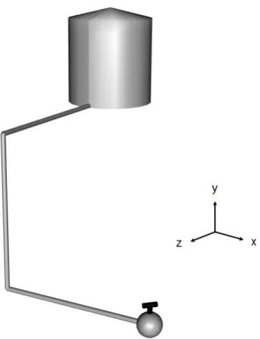
Pipe systems like the one depicted in Fig. 5 can be described by 4-DOF models. In
330
this pipe scheme, a water-hammer wave generated by the valve manoeuvre would induce
331
not only transient pressures but axial stress, shear stress and bending waves in the pipe
332
wall, hence exciting the 1,3,4,6-DOF’s.
Fig. 5: Reservoir-pipe-valve system with a 90◦ elbow at the mid-length pipe section.
Valentinet al.(1979) presented the eight-equation model for curved pipes for
1,3,4,6-334
DOF’s. Hu & Phillips (1981) solved the same equations using MOC and validated their
335
results against new experimental data. Radial inertia was included by Joung & Shin
336
(1987) who solved a nine-equation model. Tijsselinget al. (1994,1996) and Tijsseling &
337
Heinsbroek (1999) used a MOC-MOC scheme in combination with cavitation, which was
338
modelled by means of a lumped parameter model. InGale & Tiselj(2006) a FVM method
339
was used to solve the eight-equation model, which was tested for different set-ups (v.i.
340
Fig. 6). In this analysis, Gale & Tiselj (2005) highlighted that a two-phase flow model is
341
needed for simulations of more universal FSI problems occurring in pipelines.
342
Fig. 6: Numerical output fromGale & Tiselj(2006) considering a free moving valve (black dashed line), anchored (red solid line) and compared with the classic water-hammer model output (purple doted line).
A compilation of sixteen experiments dedicated to systems with a single elbow
pipes) was presented in Tijsseling (2016), eight experiments focused on the
frequency-344
domain approach and eight on the domain. The experiments based on the
time-345
domain approach are presented in Table 2.
346
Tab. 2: Main time-domain experiments carried out for single-elbow pipes.
Reference Experimental setup Transient test
Swaffield(1968–1969)
45o−180o, hor. mitre,
hor. curved bends 0.85< Rc/D <5.0,
rigid (2 jacks)
valve closure: 2 - 5 ms initial flow vel.: 0.6 - 2.4 m/s
Wood & Chao(1971) 30
o−150o, hor. mitre,
rigid and free
valve closure: 2 ms initial flow vel.: 2 - 3 m/s
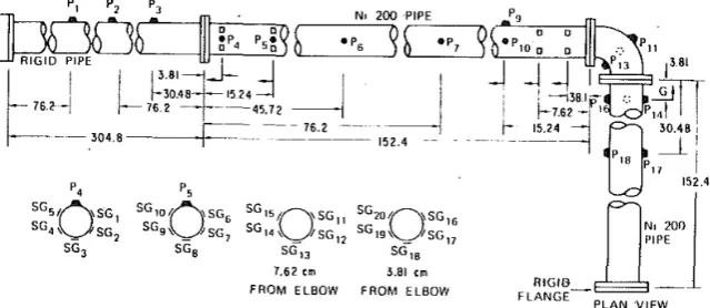
A-Moneim & Chang(1979)
hor. 114.3 mm, D= 70.6 mm, Rc/D= 1.6, rigid
gun: 150 bar pulse 3
Hu & Phillips(1981) Rc/D= 6 pellet impact 0.2 m/s Otwell(1984)
Wiggertet al. (1985b) hor. Rc/D= 0.8
valve closure: 4 ms initial flow vel.: 1.2 m/s
Tijsselinget al.(1996)
Tijsseling & Vaugrante(2001) hor. 0.88 kg rod impact 0.15 m/s
Steens & Pan(2008) hor. Rc/D= 2.2 impact hammer pulse 1 - 2 ms Altstadtet al.(2008) vert. elbowRc/D= 1.5
valve opening: 20 - 200 ms initial flow vel.: 2 - 17 m/s
Swaffield(1968–1969) tried to experimentally prove that a pressure wave reflects
par-347
tially when passing through a rigidly supported elbow. This work generated in-depth
348
discussion pointing out the importance of considering FSI even for rigid supports
as-349
suming that the movement of anchorages is nearly impossible to avoid. This idea was
350
supported by Wood & Chao (1971) who stated that pipelines are never anchored
suffi-351
ciently to eliminate motion due to a water-hammer surge. In A-Moneim & Chang (1979)
352
a complete pipe rig was used (v.i. 7), nonetheless they experimented difficulties in getting
353
rid off undesired FSI effects, emphasizing the importance of properly testing experimental
354
setups preventing such phenomena. Finally, Wiggert et al. (1985b) verified that there is
355
no pressure wave reflection from an immobile elbow but that there is due to the elbow
356
movement. InAltstadtet al. (2008) these findings were confirmed once more.
Fig. 7: Experimental pipe rig used in A-Moneim & Chang (1979).
A pipe system with multiple elbows, bends and junctions can be described by
eight-358
equation models if these are located in the very same plane. This is the case for the
359
experiment carried out in the University of Guanajuato, Mexico, in collaboration with IST,
360
Portugal. Sim˜ao et al. (2015c,b) collected data from a pipe rig assembled by concentric
361
elbows of 90◦.The apparatus was equipped with pressure transducers and accelerometers.
362
Water-hammer events were generated by a downstream valve manoeuvre. The aim of the
363
experimental data collection was the validation of a numerical model which coupled CFD
364
software for the fluid with FEM software for the structure. The model was compared
365
also with a modified MOC approach which included damping coefficients to account for
366
structural damping. The work highlighted the importance of integrated analyses including
367
the description of both fluid and structure behaviours.
368
3.6
Seven degree-of-freedom models
369
The fourteen-equation model includes all the degrees-of-freedom presented in Section 2
370
except the 2-DOF corresponding to the radial inertia of the pipe-wall, which is nested in
371
the celerity of the 1-DOF like in the classic water-hammer theory. Hence, the system to
372
be solved is composed of Eqs. 24,25,26 and 27 (i.e. the four-equation model) together
373
with Eqs. 7,8,9,10,11,12,13,14,15and 16. Pipe systems like the one depicted in Fig.
374
8 can be described by 7-DOF models, where all the related DOF’s would be excited by a
375
water-hammer wave generated at the downstream valve.
376
Wilkinson(1977) introduced the fourteen-equation model in the time-domain, which
377
was finally implemented by Wiggertet al. (1985a,1987,1985b) and Wiggert(1986) with
378
MOC approach, both in the fluid and in the structure. Experimental measurements from
379
Wiggert et al. (1987), corresponding to a similar set-up as the one depicted in Fig. 8,
380
are shown in Fig. 9. A good fitting with measurements was obtained but the analysis
381
concluded that further model developments were necessary. Lesmezet al.(1990) extended
382
the work using an experimental set-up consisting of a copper pipe containing a U-bend
383
free to move in an in-plane fashion. This method was used also byObradovi´c(1990), who
384
simulated an accident.
Fig. 8: Reservoir-pipe-valve system with two out-of-plane 90◦ elbows.
Fig. 9: Experimental pressure measurements next to the downstream valve and at a bend Wiggertet al. (1987).
Weijde(1985) carried out experiments in a PVC pipe containing a U-shaped section
386
at the laboratory of Delft Hydraulics, The Netherlands. He concluded that classic
water-387
hammer theory was not accurate enough to describe the behaviour of the pipe-rig and,
388
consequently, the FLUSTRIN project was launched. A complex and large-scale apparatus
389
(Fig. 10) held by suspension wires and specially designed for FSI tests was assembled at
Delft Hydraulics laboratory and used for the development and verification of the
FLUS-391
TRIN code, which is based on a MOC-FEM approach (Tijsseling & Lavooij,1990;Lavooij
392
& Tijsseling,1989). In this frameworkKruisbrink & Heinsbroek(1992) andHeinsbroek &
393
Kruisbrink(1993) carried out a series of numerical benchmark tests. Coupled and
uncou-394
pled Poisson effect solutions were compared for the Delft Hydraulics Benchmark Problem
395
F (Lavooij,1987), which is a good approach for verifying fourteen-equation model
imple-396
mentations (v.i. Fig. 11). Experimental measurements were used in this comparison and
397
a guideline was provided suggesting when FSI is important. The same computer code was
398
used byKruisbrink(1990),Lavooij & Tijsseling(1991) andHeinsbroek(1997) with similar
399
purposes of comparing with other modelling assumptions and using experimental tests for
400
validation. Heinsbroek(1997) suggested that for four-equation modelling an MOC-MOC
401
approach is more convenient, while for higher degrees-of-freedom an MOC-FEM scheme is
402
preferable as higher grid resolution is required. Bettinali et al. (1991) presented a similar
403
MOC-FEM code with differences in the implementation of the Poisson coupling
mecha-404
nism. Kochupillaiet al.(2005) developed a model using a velocity based FEM formulation
405
which was validated with benchmark problems. Time-domain solutions can be also
ob-406
tained from frequency-domain analyses, however, Hatfield & Wiggert (1983) concluded
407
that the time-domain solutions derived from frequency-domain results are difficult and
408
impractical.
409
a) b)
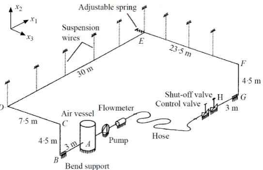
Fig. 11: Set-up of the Delft Hydraulics Benchmark Problem F (a); and numerical output (b) for: Poisson and junction coupling (solid line), only junction coupling (dashed line) and for classic water-hammer model (dash-dotted line) (Tijsseling & Lavooij, 1990).
3.7
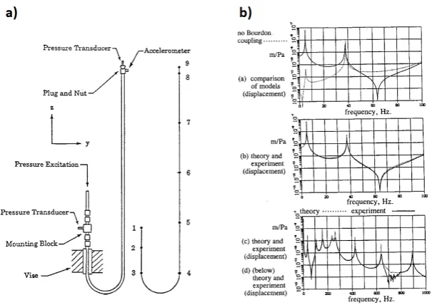
Other FSI mechanisms
410
In curved pipes of non-circular cross-section, an additional coupling mechanism, called
411
Bourdon coupling, affects the pipe behaviour. This mechanism consists of the change of
412
ovality of the pipe cross-section in function of the internal pressure loading. In Davidson
413
& Samsury(1969,1972) Fluid-Structure Interaction was analysed, respectively, in straight
414
and curved pipes. InClark & Reissner(1950) andReissneret al.(1952) the Bourdon tube
415
deformation mechanism is explained and a methodology based on the Boltzmann
super-416
position principle to describe stress-strain states is presented. Bathe & Almeida (1980,
417
1982) studied Bourdon phenomena by means of a FEM approach. The Bourdon effect was
418
first dynamically coupled with the fluid response in Tentarelli (1990). The work was
ex-419
tended in Brown & Tentarelli (2001) andTentarelli & Brown (2001), where experimental
420
measurements were used for validation of the numerical output in the frequency domain
421
(v.i. Fig.12). Budny et al.(1990) and Fan(1989) gave as well experimental evidence of
422
Bourdon coupling.
Fig. 12: Experimental set-up (a) and output in the frequency-domain (b) for Bourdon coupling analysis (Brown & Tentarelli,2001).
Other FSI mechanisms, not that common in regular engineering practices, are the
424
buckling and flutter induced by centrifugal and Coriolis forces. Authors that have
con-425
tributed on this matter are: Housner(1952),Gregory & Pa¨ıdoussis (1966), Pa¨ıdoussis &
426
Issid (1974) and Pa¨ıdoussis & Laithier(1976). Experimental research focused on
describ-427
ing the buckling and flutter effects in pipe systems was conducted inGregory & Pa¨ıdoussis
428
(1966) and Jendrzejczyk & Chen (1985).Pa¨ıdoussis (2016) gives an encyclopaedic
treat-429
ment of the subject.
430
4
Engineering applications
431
4.1
FSI consideration in codes and standards
432
Table 3 refers to the Codes and Standards belonging to those engineering fields that
433
frequently require water-hammer analyses. Other Standards and Guidelines have been
434
reviewed by Leslie & Vardy (2001). However, none of the Standards directly consider
435
any kind of FSI coupling. Several industrial cases of FSI generated by internal flows are
436
analysed in Moussou et al.(2004). The paper highlights the complexity of FSI problems
437
and the need for guidelines and rules in international Codes and Standards.
Tab. 3: Codes and Standards in industries where water-hammer analyses are frequent.
Industry Application International standards
Hydropower energy penstocks
ASME-B31.3 DIN-19704-1 ASCE MOP 79 CECT-1979
Nuclear/Thermal energy cooling systems ASME-BPV NS-G-1.9
Oil/Gas transportation oil/gas mains
ASME-B31.2 ASME-B31.4 ISO-13628
Water distribution water pipes ANSI/ASSE-1010 PDI-WH 201
Aerospace fuel pipes ISO/FDIS-8575
NASA-STD-8719
4.2
Anchor and support forces
439
Fluid-Structure Interaction and specially the behaviour of pipe supports have a direct
440
applicability in above-ground or non-buried pipe systems, such as hydropower systems,
441
long oil and gas pipes, cooling systems of nuclear, thermal plants or any fluid distribution
442
system in industrial compounds. However, only few authors investigated anchor and
443
support behaviour in the context of water-hammer theory. Frequently, studies are based on
444
qualitative discussions focused on post-accident analyses and mitigation measures
case-by-445
case oriented. An example is Almeida & Pinto (1986) where recommendations for design
446
criteria, operating rules and post-accident analyses were given. Also Hamilton & Taylor
447
(1996a,b) and Locher et al. (2000) presented qualitative discussions of the performance
448
of different industrial piping systems, giving insights of pipe supports behaviour. The
449
latter highlighted the case-by-case dependency of Fluid-Structure Interaction and the high
450
computational demand of including anchor analyses, stating that the scope of such studies
451
should be justifiable only for very critical systems, such as in nuclear power plants.
452
B¨urmann & Thielen(1988b) collected data from a firewater facility pipeline and carried
453
out numerical analyses by means of MOC. Heinsbroek & Tijsseling (1994) studied the
454
effect of support rigidity of pipe systems and discussed for what rigidity of the supports
455
FSI becomes a dominant effect. In their analysis they applied both classic water-hammer
456
theory and a MOC-FEM approach by means of the FLUSTRIN code (Lavooij & Tijsseling,
457
1989;Kruisbrink & Heinsbroek,1992). The simulated facility corresponded to the one from
458
Delft Hydraulics laboratory.
459
Tijsseling & Vardy(1996a) studied the effect of a pipe-rack considering the dry friction
460
occurring between the rack and the pipe-wall. Recommendations were given in order to
461
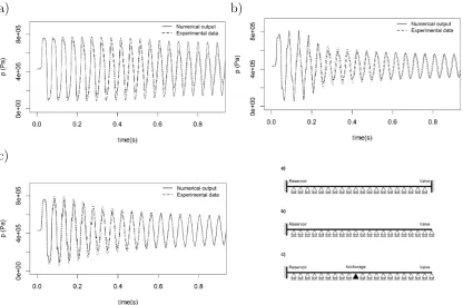
assess when dry friction must be considered. Following this line Ferras et al. (2017b);
462
Ferr`aset al. (2016a,b) carried out experimental and numerical work based on a straight
copper pipe which allowed a broad variety of anchoring configurations. In Ferras et al.
464
(2017b) a robust and accurate MOC-MOC code to simulate anchoring blocks taking into
465
account their inertia and dry friction is presented. The blocks were nested in the numerical
466
scheme as internal conditions and junction coupling was considered. Fig. 13 depicts the
467
model output vs. experimental measurements for different anchoring set-ups.
468
a) b)
c)
Fig. 13: Validation of the numerical model developed inFerraset al.(2017b) for: anchored pipe ends (a); released downstream end (b); and released downstream end but anchored midstream (c).
Different anchoring conditions were assessed in Sim˜ao et al. (2015c) using CFD
soft-469
ware, which was validated by means of experimental data. The analysis pointed out the
470
need of CFD simulations for the proper description of pipe supports behaviour. In
Zan-471
ganeh et al. (2015) the aim was the simulation of hydraulic transients in a straight pipe
472
anchored with axial supports using a MOC-FEM approach. Both pipe-wall and supports
473
had a viscoelastic behaviour. The study concluded that the viscoelastic supports
sig-474
nificantly reduce displacements and stresses in the pipe and eliminate the high frequency
475
fluctuations produced due to FSI. InWu & Shih(2001) andYanget al.(2004) a multi-span
476
pipe system, with middle rigid constraints was analysed in the frequency-domain using
477
the transfer matrix method, concluding that the middle rigid constraints have a much
478
larger effect than the Poisson coupling. These types of multi-span pipes with middle rigid
479
constraints set-ups are common in engineering practices and, so far, only a limited
ber of investigations has been carried out addressing this issue, especially in time-domain
481
analyses.
482
4.3
Vibration damping and noise reduction
483
Pipe vibration may induce audible noise and FSI analyses are required for the
assess-484
ment of such noise. Moser et al. (1986) investigated the vibrating modes that produce
485
sound. Kwong & Edge (1996, 1998) carried out experimental analyses and developed a
486
technique to reduce noise generation by the specific positioning of pipe clamps. De Jong
487
(1994) suggested that for the full description of sound generation in pipe-systems, seven
488
degrees-of-freedom are required. This statement was verified in Janssens et al. (1999).
489
InChen (2012) a pump-induced fluid-borne noise investigation is carried out by means of
490
a distributed-parameter transfer-matrix model in the frequency-domain. It was claimed
491
that the method could be used as well for structure-born noise as long as Fluid-Structure
492
Interaction was taken into account.
493
Tijsseling & Vardy (1996b) carried out experimental water-hammer tests on a steel
494
pipe containing a short segment of ABS. MOC was successfully used to reproduce the
495
experiments and they concluded that the vibration could be adapted and modified in
496
function of the segment material and geometry. Hachem & Schleiss(2012) reached a similar
497
conclusion in an aluminium pipe set-up with a short segment of PVC. The analysis was
498
carried out in the frequency-domain. Related with the previous subsection, Koo & Park
499
(1998) proposed a methodology to reduce vibrations by the installation of intermediate
500
supports.
501
4.4
Earthquake engineering
502
Water-hammer waves can be produced by earthquake excitation on a pipe system.
Fluid-503
Structure Interaction or soil-pipe interaction may be one of the potential damaging factors
504
during earthquakes, specially for relatively low pressure and large diameter pipelines (Young
505
& Hunter,1979). The Fukushima Daiichi nuclear disaster in Japan is a prominent example
506
of this (Lo Frano & Forasassi, 2012; Mitsume et al., 2014). Some authors have studied
507
this kind of transients coupled with FSI. Hara (1988) analysed a Z-shaped piping
sys-508
tem subjected to a one-directional seismic excitation. A numerical analysis of a 3D pipe
509
system was carried out in Hatfield & Wiggert (1990). It was found that assuming the
510
piping to be rigid produced an upper-bound estimate of pressure, but assuming the liquid
511
to be incompressible resulted in underestimating the displacement of the piping.
Cou-512
pled and uncoupled analyses applied to a single straight pipe were compared in Bettinali
513
et al. (1991), who also concluded that coupled analyses accurately predicted lower wave
514
amplitudes.
4.5
Aerospace engineering
516
Strong fluid transients occur in the filling up process of propulsion feedlines of satellites and
517
launchers. In the experimental works of Regetz (1960), Bladeet al. (1962),A-Moneim &
518
Chang (1978) andA-Moneim & Chang(1979) different configurations of rocket fuel-filled
519
pipe rigs were tested. An overview of the main concerns experienced in the aerospace
com-520
munity with respect to fluid-hammer is reported by Steelant (2015). The study remarks
521
the need of detailed investigation of Fluid-Structure Interaction in combination with
ther-522
mal heat transfer during fluid-hammer waves in satellites or launchers. Bombardieriet al.
523
(2014) also highlight the importance of FSI in the filling of pipelines during the start up
524
of the propulsion systems of spacecrafts, claiming that more experimental research should
525
be focused on this line.
526
4.6
Biomechanics
527
The disciplines of hydraulic transients and physiological flows share a good basis of the
528
classic water-hammer theory as long as the assumptions of liquids with relatively low
com-529
pressibility contained in thin-walled elastic cylindrical tubes are considered. Studies such
530
as Lambossy (1950), McDonald (1974), Nakoryakov et al. (1976), Anderson & Johnson
531
(1990), Sherwin et al. (2003), Van de Vosse & Stergiopulos (2011), Nichols et al. (2011)
532
and Alastrueyet al.(2012) focused on adapting classic water-hammer to the main factors
533
that affect physiological flows. For instance, inAnderson & Johnson(1990), the Korteweg
534
formula for wave celerity computation was reviewed in order to include pipe cross-section
535
ovality effects. The study concluded that even for a low ovality of the pipe cross-section
536
there may be significant reductions of the wave velocity due to bending-induced changes in
537
the tube cross-section. The analysis carried out byAnderson & Johnson(1990) serves also
538
in the field of hydraulic transients for pipe bends and coils where the pipe cross-section
539
becomes elliptic.
540
Nowadays, computational-fluid-dynamics (CFD) tools are used to model the
complex-541
ity of haemodynamics. Not just the pipe-wall viscoelasticity and the elliptic pipe
cross-542
section, but the inner fluid defies as well classic water-hammer theory assumptions as blood
543
is a non-Newtonian fluid, presenting shear-thinning, viscoelasticity and thixotropy.
Wa-544
thenet al. (2009) presents a review of modern modelling approaches for haemodynamical
545
flows. InJanelaet al.(2010) a comparison of different physiological assumptions is carried
546
out by means of a FEM-FEM approach. Newtonian and non-Newtonian assumptions are
547
considered with Fluid-Structure Interaction, highlighting their differences and the
impor-548
tance of good modelling criteria. More specific to blood flow diseases diagnoses, Sim˜ao
549
et al. (2016a) also used CFD tools, including FSI, for modelling a vein blockage induced
550
by a deep venous thrombosis and the occurrence of reverse flow in human veins.
551
4.7
Accidents and post-accident analyses
552
FSI may generate overpressures higher than that predicted by Joukowsky’s formula and
553
not only caused by water-hammer waves, but also by turbulence-induced vibrations,
cavitation-induced vibrations or vortex shedding with lock-in. These phenomena are
555
poorly understood (Moussou et al., 2004) and are rarely taken explicitly into
consider-556
ation in engineering designs, leading to accidents and service disruptions of important
557
infrastructure with large social relevance (e.g. industrial compounds, water and
wastew-558
ater treatment plants, thermal plants, nuclear power plants, hydropower plants).
559
Jaeger et al. (1948) reviewed a number of the most serious accidents due to
water-560
hammer in pressure conduits until WWII. Many of the failures described were related to
561
vibration, resonance and auto-oscillation (Bergant et al., 2006). Table 4 summarizes a
562
selection of accidents caused by strong hydraulic transients found in the literature, noting
563
that the majority of incidents and accidents remains ‘unpublished’.
564
Normally, accidents in hydraulic facilities are associated not only to a single
phe-565
nomenon but to a sequence of events that make the system collapse. Although not all the
566
accidents listed in Table 4 were caused directly by FSI, in many cases FSI is involved in
567
this sequence of events and its understanding is crucial in post-accident analyses, such as
568
reported inAlmeida & Pinto(1986),Wanget al.(1989),Obradovi´c(1990) andSim˜aoet al.
569
(2016b). Leishear (2017) investigated water-hammer related accidents in nuclear power
570
plants, where water-hammer waves compress flammable gasses to their autoignition
tem-571
peratures in piping systems. In this paper several examples of incidents and accidents are
572
analysed enhancing the understanding of nuclear power plant explosions.
Tab. 4: Selection of historical accidents in pressurized pipe systems mentioned in the lit-erature.
Location Facility Description and citations
Oigawa,
Japan Penstock
A water-hammer wave, caused by a fast valve-closure, split the penstock open and produced the pipe collapse upstream.
Bonin(1960). Big Creek,
U.S.A. Penstock
Burst turbine inlet valve caused by a fast closure.
Trenkle(1979). Azambuja,
Portugal Pump station
Collapse of water column separation causing the burst of the pump casing.
Chaudhry(2014) L¨utschinen,
Switzerland Penstock
Penstock failure during draining due to the buckling produced by a frozen vent at the upstream end.
Chaudhry(2014). Arequipa,
Peru Penstock
The clogging of the control system of a valve resulted in buckling and the failure of the welding seams of the penstock due to fatigue.
Chaudhry(2014) Ok,
Papua New Guinea Power house
The draft tube access doors were damaged and the power house flooded due to column
separation in the system.
Chaudhry(2014). Lisbon,
Portugal Water main
Rupture of concrete support blocks during the slow closure of an isolation valve installed in a large suction pipe.
Almeida & Ramos(2010);Sim˜aoet al.(2016b). New York,
U.S.A. Steam pipe
Condensation-induced water-hammer caused the rupture of the steam pipe.
Vecchioet al.(2015) Lapino,
Poland Penstock
Burst of the penstock caused by a rapid cut-off and low quality of the facility.
Adamkowski(2001). Chernobyl,
Ukraine Nuclear reactor
Fuel pin failure, fuel-coolant interaction and Fluid-Structure Interaction were involved in the failure of the nuclear reactor.
Wanget al.(1989). New York,
U.S.A Nuclear reactor
Circumferential weld failure in one of the feedwater lines due to a steam generator water-hammer.
5
Conclusions
574
Not considering pipe-wall movement during water-hammer events is going against the
575
essence of water-hammer research. As shown in Appendix B, the classic water-hammer
576
equations assume a quasi-steady circumferential deformation of the pipe-wall. The
infor-577
mation of this quasi-steady behaviour of the piping structure affecting the pressure wave
578
is, in the classic approach, enclosed in the water-hammer wave celerity, which may be
even-579
tually affected, as well, if other pipe degree-of-freedoms are considered. Jumping from this
580
quasi-steady assumption of the pipe structure to an unsteady one is what makes the trade
581
between the fluid and the structure dynamic; Fluid-Structure Interaction arises and the
582
classic water-hammer theory becomes invalid. Even in very well controlled conditions of
583
hydraulic laboratories, undesired FSI phenomena are frequent. An important challenge
584
of experimental research in FSI is the setting up of the right design to fit the research
585
purpose. Validation of the test rig itself is, therefore, crucial.
586
Fluid-Structure Interaction is a case-dependent problem; there is no general solution
587
or numerical model capable of describing and simulating any pipe setup. The technical
588
challenge in the scope of 1D FSI is not resolving the fundamental equations, but assuming
589
the appropriate coupling between the different pipe degrees-of-freedom without ending up
590
in expensive computations. This case-dependency feature and the lack of user-friendly
591
tools is what makes FSI problems difficult to tackle in engineering practice. Additionally,
592
there is a general consuetudinary thinking that classical approaches remain on the
conser-593
vative side. Though, in this review, it has been shown how authors demonstrated, both
594
numerically and experimentally, that FSI may generate overpressures higher than ones
595
estimated by the classical solutions. Moreover, there is no engineering code or standard
596
specifying when FSI has to be considered. All these factors pinpoint that the physics of
597
FSI phenomena are not fully understood in common engineering practices and this involves
598
the potential risk of underrated designs.
599
Acknowledgements
600
This research is supported by the Portuguese Foundation for Science
601
and Technology (Funda¸c˜ao para a Ciˆencia e a Tecnologia) through the
602
project ref. PTDC/ECM/112868/2009 “Friction and mechanical energy
603
dissipation in pressurized transient flows: conceptual and experimental
604
analysis”, the PhD grant ref. SFRH/BD/51932/2012 also issued by
605
FCT under IST-EPFL joint PhD initiative and by the Swiss Competence
606
Center for Energy and Research-Supply of Electricity (SCCER-SoE).
References
608
A-Moneim, M. & Chang, Y.(1978). Comparison of Icepel code predictions with straight 609
flexible pipe experiments. Nuclear Engineering and Design 49(1), 187–196.
610
A-Moneim, M. & Chang, Y.(1979). Comparison of Icepel predictions with single-elbow 611
flexible piping system experiment. Journal of Pressure Vessel Technology 101(2), 142–
612
148.
613
Adamkowski, A. (2001). Case study: Lapino powerplant penstock failure. Journal of 614
Hydraulic Engineering 127(7), 547–555.
615
Alastruey, J., Parker, K. H. & Sherwin, S. J. (2012). Arterial pulse wave haemo-616
dynamics. In: 11th International Conference on Pressure Surges. Virtual PiE Led t/a
617
BHR Group.
618
Allievi, L. (1902). Teoria generale del moto perturbato dell’acqua nei tubi in pressione 619
(colpo d’ariete). Translated into English by EE Halmos (1925). American Society of
620
Civil Engineers .
621
Almeida, A. & Pinto, A.(1986). A special case of transient forces on pipeline supports 622
due to water hammer effects. In: Proceedings of the 5th International Conference on
623
Pressure Surges, Hanover, Germany, vol. 2224.
624
Almeida, A. & Ramos, H. (2010). Water supply operation: diagnosis and reliabil-625
ity analysis in a Lisbon pumping system. Journal of Water Supply: Research and
626
Technology-Aqua 59(1), 66–78.
627
Altstadt, E., Carl, H., Prasser, H. & WeiB, R.(2008). Fluid-Structure Interaction 628
during artificially induced water hammers in a tube with a bend – Experiments and
629
analyses. Multiphase Science and Technology 20(3–4), 213–238.
630
Anderson, A.(1976). Menabreas note on waterhammer: 1858.Journal of the Hydraulics 631
Division 102(1), 29–39.
632
Anderson, A. & Johnson, G. (1990). Effect of tube ovalling on pressure wave
propa-633
gation speed. Proceedings of the Institution of Mechanical Engineers, Part H: Journal
634
of Engineering in Medicine 204(4), 245–251.
635
Barez, F., Goldsmith, W. & Sackman, J. (1979). Longitudinal waves in liquid-filled 636
tubes I: Theory. International Journal of Mechanical Sciences 21(4), 213–221.
637
Bathe, K. & Almeida, C. (1980). A simple and effective pipe elbow element-linear 638
analysis. Journal of Applied Mechanics 47(1), 93–100.
639
Bathe, K. & Almeida, C.(1982). A simple and effective pipe elbow element-interaction 640
effects. Journal of Applied Mechanics 49(1), 165–171.
Belytschko, T., Karabin, M. & Lin, J. (1986). Fluid-Structure Interaction in wa-642
terhammer response of flexible piping. Journal of Pressure Vessel Technology 108(3),
643
249–255.
644
Bergant, A., Simpson, A. R. & Tijsseling, A. S. (2006). Water hammer with 645
column separation: a review of research in the twentieth century. Journal of Fluids and
646
Structures 22(2), 135–171.
647
Bettinali, F., Molinaro, P., Ciccotelli, M. & Micelotta, A. (1991). Transient 648
analysis in piping networks including Fluid-Structure Interaction and cavitation effects.
649
Transactions SMiRT 11, 565–570.
650
Bietenbeck, F., Petruschke, W. & Wuennenberg, H.(1985). Piping response due
651
to blowdown significant parameters for a comparison of experimental and analytical
652
results. In: Transactions of the 8th International Conference on Structural Mechanics
653
in Reactor Technology. Vol. F1 and F2.
654
Blade, R. J., Lewis, W. & Goodykoontz, J. H. (1962). Study of a sinusoidally 655
perturbed flow in a line including a 90 degree elbow with flexible supports. National
656
Aeronautics and Space Administration (NASA), Lewis Research Center, Cleveland,
657
Ohio.
658
Bombardieri, C., Traudt, T. & Manfletti, C.(2014). Experimental and numerical 659
analysis of water hammer during the filling process of pipelines. In: Space Propulsion
660
Conference, Cologne, Germany.
661
Bonin, C. (1960). Water-hammer damage to Oigawa power station. Journal of Engi-662
neering for Power 82(2), 111–116.
663
Borzi, A. & Propst, G. (2003). Numerical investigation of the Liebau phenomenon. 664
Zeitschrift f¨ur angewandte Mathematik und Physik ZAMP 54(6), 1050–1072.
665
Bouabdallah, S. & Massouh, F. (1997). Fluid-Structure Interaction in hydraulic 666
networks. American Society of Mechanical Engineers. Aerospace Division Newsletter
667
AD-53-2, 543–548.
668
Boulanger, A. (1913). Etude sur la propagation des on