Article
1
Thermal and Electrical parameter identification of a
2
Proton Exchange Membrane fuel cell using genetic
3
algorithm
4
H. Eduardo Ariza 1, Antonio Correcher 2, Carlos Sánchez 3, Ángel Navarro-Pérez4 and Emilio
5
García5
6
1 Corporación Universitaria Comfacauca; [email protected]
7
2 Universitat Politècnica de València; [email protected]
8
3 Universitat Politècnica de València; [email protected]
9
4 Universitat Politècnica de València; [email protected]
10
5 Universitat Politècnica de València; [email protected]
11
12
13
Abstract: PEM fuel cell is a technology successfully used in the production of energy from
14
hydrogen, allowing the use of hydrogen as an energy vector. It is scalable for stationary and
15
mobile applications. However, the technology demands more research. An important research
16
topic is fault diagnosis and condition monitoring to improve the life and the efficiency and to
17
reduce the operation costs of PEMFC devices. Consequently, there is a need of physical
18
models that let deep analysis. These models must be accurate enough to represent the PEMFC
19
behavior and to allow the identification of different internal signals of a PEM fuel cell. This
20
work presents a PEM fuel cell model that uses the output temperature in a closed loop, so it
21
can represent the thermal and the electrical behavior. The model is used to represent a NEXA
22
Ballard 1.2 kW; therefore it is necessary to fit the coefficients to represent the real behavior.
23
Five optimization algorithms were tested to fit the model, three of them were taken from
24
literature and two were proposed. Finally, the model with the parameters identified was
25
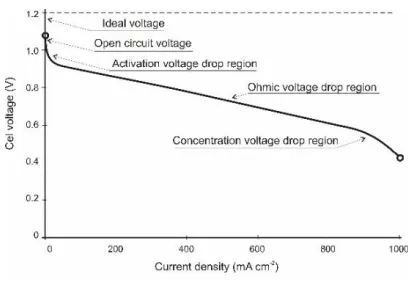
validated with real.
26
Keywords: PEM fuel cell; identification; Genetic algorithm; Model; LabVIEW
27
28
1. Introduction
29
Proton Membrane Exchange Fuel Cell (PEMFC) is an electrochemical device, which is able to
30
convert chemical energy (stored hydrogen) into electrical energy. PEMFC is an interesting power
31
source solution due to its low operation temperature, its high power density, its good response to
32
varying loads, and its easy scale-up [1] . However, the high cost of this technology makes modelling,
33
parametric identification and fault diagnosis necessary research topics to improve the use of PEMFC
34
[2]. PEMFCs have parameters that change from one cell to another because of different reasons:
35
manufacturing materials, physical dimensions, aging, working conditions, etc. Adequate cell
36
identification is necessary to know the internal cell conditions, to define the optimal working point,
37
to estimate the supply power capacity, and to implement condition monitoring techniques or fault
38
diagnosis algorithms. More complete, detailed and accuracy models allow the detection of small
39
variations that can be considered as preludes of possible failures. Detecting these variations could
40
prevent irreparable damages, it will lower replacement costs, and it will improve the reliability of
41
the system.
42
There are some previous works dealing with PEMFC model identification. Each approach
43
includes its own model structure and simplifications. Regarding the identification techniques, they
44
are highly dependent on the PEMFC model and they can be classified into two big subsets: static
45
models and dynamic models.
46
The static model is created to identify the cell polarization curve in specific conditions of
47
pressure and temperature. Hence, the experiment must keep as constants these variables.
48
49
Figure 1 shows a typical cell polarization curve which represents the main cell characteristics.
50
As the current increases the voltage drops in three visible sections: the first voltage drop represents
51
cell activation losses; the second section represents voltage losses by internal resistance, and the
52
third section represents the voltage drop by gas transportation or concentration losses [3].
53
54
55
Figure 1 Typical PEMFC polarization curve
56
In [4] a model based on Neural Networks and used the Levenberg-Marquardt BP algorithm to
57
identify the polarization curve characteristics is proposed. The model inputs were the airflow and
58
the temperature, and the outputs signals were the current and voltage. The model presented good
59
accuracy; however, the system demanded training with high computational cost, and the authors
60
exposed as an alternative the use of other Optimization algorithms (OA).
61
The identification of equations based in the model [5] and using OA is a clear tendency, these
62
models have electrical and thermodynamics equations with around seven coefficients which allow
63
tuning the model. The coefficients are identified using an optimization function which minimizes
64
the error between simulated and real signals. In [6] the current demand is used as input to generate
65
de polarization curve. The identification of the coefficients was performed with an OA called Hybrid
66
Genetic Algorithm (HGA) that avoids the premature convergence of Simple genetic algorithms
67
(SGA). The HGA needs to be fed with parameters closer to ideal values previously identified. In [7] a
68
similar model to the previous one was used to identify the system with a Particle swarm
69
optimization algorithm (PSO) as an algorithm which accepts initial parameters located in a very
70
broad range. In [8] is presented a Grouping-based global harmony search algorithm (GGHS) to
71
surpass the limits of Harmony search algorithm (HS). This work compared the GGHS with versions
72
of HG and PSO, and concluded that the GGHS overcomes the mentioned algorithms. The
73
Grasshopper Optimization Algorithm (GOA) was proposed by [9] to identify the parameters of
74
three different PEMFC, Though, GGHS and GOA require that the initial parameters fall within
75
modification of PSO that makes the algorithm configuration be dynamic to avoid finds fake
77
solutions is proposed. However, this modification increases the computational cost in regarding to a
78
PSO. To overcoming the mentioned problems of PSO, in [11] a Grey Wolf Optimizer is proposed,
79
this algorithm was tested with the classical model and five real different PEMFC. Related to
80
differential evolution (DE) algorithm framework, some author proposed variations to improve the
81
performance of the scaling factor F. in [12] proposed the hybrid adaptive differential evolution
82
algorithm (HADE) and they compared it with PSO and two versions of differential evolutionary
83
algorithms is proposed. The HADE overpasses the performance of the others OA in terms of
84
minimization velocity. The comparison was made using test functions, but the PEMFC model and its
85
optimization function only was carry out whit HADE. Transferred adaptive DE (TRADE) is an DE
86
improve algorithm applied to a PEMFC and SOFC models proposed by [13]. Though, GGHS and
87
GOA require that the initial parameters fall within closer bounds both presents attractive results. On
88
the similar way, [14] proposed a hybridization between Teaching Learning Based Optimization
89
method (TLBO) and DE algorithm, this application lets obtain better results with low computational
90
cost, compared with single TLBO and DE separately. In [15] the quantum-based optimization
91
method (QBOM) applied to the identification of three voltage drop coefficients of a NEXA 1.2 kW
92
PEMFC model is introduced. QBOM showed good accuracy and high minimization velocity in the
93
identification. However it was applied in the identification of three parameters versus the seven
94
parameters identified by previously mentioned works.
95
The above authors demonstrated the usefulness of OAs to parameter identification of PEMFC
96
polarization curves. Moreover, the PEMFC polarization curve only represents the cell operation at
97
one single stack temperature value and a single stable pressure of inlet gasses.
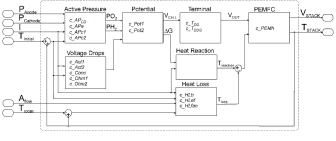
98
In the second main classification are the dynamic PEMFC models. Those models represent
99
better the real behavior of a PEMFC because they show changes in the cell response when there are
100
changes on the load current and other variables and consider the cell as a Multiple-input
101
multiple-output system (MIMO). Each identification technique uses particular excitation inputs
102
(such as steps, ramps or waves) and each one uses the outputs to build or to adjust transfer functions
103
or state space models which include the fuel cell parameters. To facilitate the model identification,
104
some PEMFC models can also be simplified by working with constant temperatures or by using
105
linearization techniques.
106
A dynamic model used to test several control strategies was presented in [16]. This model
107
included inputs such as: inlet molar flow rates of oxygen and hydrogen; inlet temperatures of anode
108
and cathode gas; and inlet coolant flow rate. After the excitation with input steps, the authors
109
developed an empirical identification by monitoring the average power density and the average
110
solid temperature. In [17] the authors used transfer functions to model a PEMFC. This work used the
111
stack current and the cathode oxygen flow rate as inputs and the stack voltage and the cathode total
112
pressure as outputs. The model is able to predict the output signals near to the operation point. In
113
[18], a PEMFC Hammerstein model is presented. The inputs were current, stoichiometric oxygen,
114
and cooling water flow, and the outputs were the partial pressure of O2 and the stack temperature.
115
The identification process used different random steps signals as inputs. In [19] a PEMFC dynamic
116
model that included the polarization curve characteristics and a double layer charge effect is
117
proposed. The model input was a typical current demand of a DC-DC or a DC-AC. In [20] a
118
NARMAX model to represent the MIMO relations and to identify the coefficients satisfying the
119
PEMFC voltage simulation is used. Also a NARMAX model is used by [21] to represent PEM and
120
used a GA to the model identification, however, the model only represents the fuel cell temperature.
121
Buchlozt and Krebs [22] splits the PEMFC model into a dynamic part and a static part. The static
122
model was identified with Neural Networks whereas the dynamic model was developed with a mix
123
of transfer functions and linear state-space models. The model inputs were: current density, oxygen
124
stoichiometry, gas supply pressure, and gasses relative humidity; other values as stoichiometry of
125
oxygen and stack temperature were set to constant. The model output was the sum of the dynamic
126
and the static voltage. The authors exposed that the split model allows to reduce the computational
127
part, the inputs were the current and the cathode pressure. All these works get deeper in the
129
different relationships between input and output signals, so they model cell voltage responses to
130
gasses pressures and current variations. Nevertheless, PEMFC operation produces heat that changes
131
in the cell temperature. The temperature affects the cell performance and features as open circuit
132
voltage, internal gasses pressures, gas humidity, and internal resistances. Therefore, the use of
133
temperature as an input variable will give more accuracy to the model despite de fact that the
134
increment of complexity and nonlinearity.
135
Wang et al. [24] developed a dynamic equations model where the temperature is considered to
136
work in closed loop. The model included the electrochemical and thermal responses and the cell
137
double layer charge effect, and has a good response in steady state and transients. The model
138
characteristics are applicable in fault diagnosis and condition monitoring tasks; thus, this work was
139
developed for a 500 W PEMFC and is not directly usable for other devices.
140
One recent approach [25] used an equivalent electrical circuit model to represent a Nexa Ballard
141
1.2Kw PEMFC. This model simulated both the output voltage and the stack temperature. The model
142
included fourteen electric coefficients and six thermal coefficients. They were identified with an
143
Evolution strategy algorithm (ES). This work showed a model that includes the stack thermal
144
dynamics and they applied GA to the parameter identification, however, the thermal model includes
145
a piecewise heuristic function to link the temperature with the current to adjust the operation of the
146
cooling system of the real cell. This last component and the model based on electrical circuit do not
147
let access to internal signals system. Salim et al. [26] use equations based model which includes the
148
thermal behavior of NEXA 1.2kW PEMFC. The voltage model was developed by a fitting
149
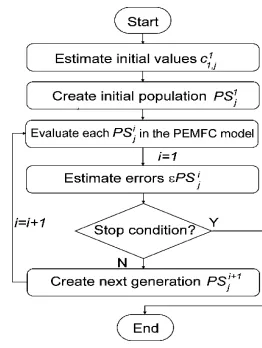
polynomial curve which involves the classical voltage losses. The thermal model was developed
150
using the sensible heat and latent heat. The identification process applies PSO with one independent
151
optimization function for the voltage part and other for the thermal model. The result shows high
152
simulation accuracy. However, the model does not take into account the temperature in a closed
153
loop, neither the cooling system performance of the device.
154
155
Figure 2 Block diagram of Nexa fuel cell balance of plant.
156
The present work is involved in a wider study related with fault diagnosis and condition
157
monitoring of a Nexa Ballard 1.2kW PEMFC installed in the Laboratory of Distributed Energy
158
Resources [27]. Figure 2 shows the block diagram of the complete Nexa system. Hydrogen is
159
supplied from a compressed tank at adequate pressure. Reaction air is supplied by means a
160
compressor and measured by a mass flow meter. Temperature is measured at the air outlet, so this is
161
the stack temperature. The system is cooled by a fan in order to maintain the temperature under the
162
upper limit. Voltage of the complete stack and the last two cells is measured in order to determine
163
when the hydrogen purge valve is opened to eliminate accumulated impurities. Current generated
164
by the fuel cell is measured for two reasons: to open the relay if current exceeds the maximum and to
165
act over the air compressor to maintain the correct stoichiometric relationship. Table 1 shows the
166
manufacturer values of the PEMFC.
167
Table 1 Maximum characteristics of Nexa 1200 fuel cell
169
Power 1200 W
Operating voltage range 22 – 50 V
Current 55 A
Hydrogen consumption 18.5 slpm
Air flow 90 slpm
Temperature 80 oC
Cooling air flow 3600 slpm
170
The overall study requires a model able to represent the device and that uses the maximum
171
amount of measured data. In addition, the identification process must be accurate, fast, and with the
172
lowest computational cost as possible to make the model suitable to be used in real time
173
applications. This paper uses the model presented by [24] to fit the NEXA 1.2kW PEMFC real data.
174
Moreover, several GA are used and they are compared in order to look for the best strategy to fit the
175
model.
176
Section 2 shows the description of the model. Section three shows the adjustment of the
177
equations coefficients to fit the PEMFC Nexa behavior. The results of the identification and the
178
model validation are presented in section four. Finally, we present some conclusions and future
179
works.
180
2. The PEMFC model
181
Materials The model presented in this paper is an extension of the dynamic model
182
presented in [24] where explained the model in detail. This work only presents the key
183
equations and the modifications included. The model was originally created to represent a
184
500W PEMFC and it was implemented with Matlab/Simulink® and Pspice®. However, the
185
Nexa 1.2kW PEMFC software (NexaMon OEM 2.0) gives more information as inlet pressures
186
and cooling system variables that can be taken into account to model the thermal development
187
of the fuel cell. Figure 3 shows PEMFC model, including the in/out put signals.
188
189
Figure 3 PEMFC model
190
The model is grouped into electrical and thermal equation sets. The most remarkable
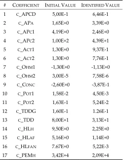
191
variable in the electrical set is the cell potential Ecell(t) which is calculated with the Nernst’s
192
equation. Equation (1) is a simplification of the Nernst’s equation which assumes: a) the Stack
193
keeps under 100º C its temperature; b) the reaction product is in a liquid phase. The equation
194
includes a voltage Ed,cell(t) which represents the electrical effect of gas pressure changes during
195
load transients and classical voltage drops.
196
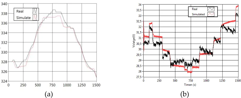
197
E (t) = E (t) + R · T(t)
2 · F · ln[p
∗ (t) · (p∗ (t)) . ] − E
Where T(t) is the cell temperature (K); F is the Faraday constant (96487 coulombs/mol); R is
198
the ideal gas constant (8.3143 J/mol K); E0(t) is the reference potential at standard conditions
199
(298 K, 1 atm); pH2*(t) is the H2 effective partial pressure; pO2*(t) is the O2 partial pressure.
200
Ed,cell(t) is initially modelled in Laplace domain as equation (2) and implemented in time
201
domain equation (3).
202
, = · ( ) · + 1 (2)
, = ·
·
+ ( ) (3)
203
Where I(t) is the current (A); p is the simulation step; d, τ are a delay constants related to
204
PEMFC distribution layers.
205
Regarding the thermal equations set, the thermal loss equation was modified to include the
206
cooling system of Nexa PEMFC. It is identified in the equation (4).
207
208
̇ ( ) = ℎ ( ) · ( ) + ( ) · · · ( ) (4)
Where, hcell is the convective heat transfer coefficient (W/m2·K) of the stack; Ncell is the
209
number of cells in the stack; Acell is the cell area (cm2). The control system of a Nexa includes the
210
operation of a fan and cooling system, providing oxygen inlet and keeping the temperature
211
under a limit to keep operation conditions and avoid membrane damage. Af (t) is a coefficient to
212
adjust the temperature related to the cooling system.
213
The proposed model has been split into functional blocks (Figure 3), so each block can be
214
analyzed separately for fault diagnosis purposes. Each block contains tunable coefficients to
215
reduce the difference between the real and the simulated signals. The blocks and its respective
216
coefficients are described bellow:
217
218
Active pressure block calculates the effective partial pressure in the anode and the cathode
219
side. The block has four parameters
220
c_APCD is a parameter related to the cell current density.
221
c_APa is a parameter related to the distance between the anode channel and the catalyst
222
surface.
223
c_APc1 is a parameter related to the distance between the cathode channel and the catalyst
224
surface.
225
c_APc2 is a parameter that fits the pressure of saturated H2O curve in function of the
226
temperature.
227
228
Voltage drop block represents the voltage losses by activation, internal resistance, and
229
concentration. The coefficients are:
230
c_Act1 is a parameter related to the activation voltage drop that only depends on temperature.
231
c_Act2 is a parameter related to the activation voltage drop, that depends on current and
232
temperature.
233
c_Ohm1 is the parameter related to ohmic losses that depends on current and temperature.
234
c_Ohm2 is a parameter related to ohmic losses that only depends on cur- rent.
235
c_Conc is a parameter related to the voltage concentration drop.
236
237
The potential of the cell are calculated in the Potential Block which includes two coefficients:
238
c_Pot1 is a value that adjusts the internal electric potential of the cell.
239
c_Pot2 is a parameter related to the free Gibbs energy (∆G).
240
The Terminal Block represents the electrical global stack behavior. This block includes the cell
242
potential, the voltage losses, and a voltage drop by fuel and oxidant delays during load transients.
243
The Terminal Block has the following parameters:
244
c_TDD is the gasses delay time constant during load transients.
245
c_TDDG represents a gain that affects the delay by load transients.
246
247
The Heat Loss block represents thermal losses that leave the stack by air convection and energy
248
absorbed by exhaust gasses. The parameters are:
249
c_HLh is a gain that affect the overall heat loss.
250
c_HLaf is the parameter fitting the thermal loss associated to the cathode side. It is included in
251
the stack thermal loss.
252
c_HLfan is a gain associated with the cooling fan system and it is included in the stack thermal
253
loss.
254
255
PEM Block merges the electrical and the thermal equations to represent the global PEMFC
256
performance. This block has one parameter.
257
c_PEMh is related to the total mass of stack and its overall specific heat capacity.
258
259
A complete set of parameters (PS) can be used to simulate the PEMFC. Therefore, the goal of
260
this research will be the search of the set of parameters that minimizes the difference between the
261
PEMFC real outputs and the model outputs. The notation used to define the different elements of
262
the algorithms is presented below:
263
264
PS = {c_APCD, c_APa, c_APc1, c_APc2, c_Act1, c_Act2, c_Ohm1, c_Ohm2,
265
c_Conc, c_Pot1, c_Pot2, c_TDD, c_TDDG, c_HLh, c_HLaf, c_HLfan, c_PEMh}
266
267
A population of parameter sets (an array of parameter sets) will be noted as:
268
269
PS = PS , PS , PS , … , PS
270
Where PSk is the population of kth iteration.
271
272
PS = c ,, c ,, c ,, … , c ,
273
Where PSjk is jth parameter set of the kth population and the ith model parameter will be noted as
274
c ki,j. For example, c71,2 corresponds with the value of parameter 1 c_APCD in parameter set 2 of the
275
7th population.
276
The model was programmed and tested with initial coefficients taken from [24] and from the
277
device manufacturer manual. This PEMFC model was simulated using real inputs signals. Figure 4
278
shows the predicted voltage and temperature as well as the real values. Therefore, despite the fact
279
that there is a significant difference, the model seems to be suitable to represent the system dynamics
280
after a suitable parameter fitting. The MSE obtained with the initial coefficients represent a challenge
281
in the identification process because huge starting errors make it difficult to find the optimal
282
parameter set.
283
(a)
(b)
Figure 4 Model test using the initial parameters: (a) stack temperature; (b) output voltage
285
286
3. Parameter identification
287
288
shows the identification process. The process begins with the generation of a randomized
289
population.
290
291
292
Figure 5 Global identification process algorithm
293
This population is created from an initial PS11 as indicated in equation (5)
294
295
= = 1: , = ,
≥ 1: , = , · · + ,
(5)
296
Where z is a random number in the range [-1, 1] and vd is a value to generate initial dispersion1.
297
Each PSk is simulated with real inputs and its corresponding error is shown in equation (6).
298
299
= +
2 (6)
300
Where εV is the output voltage error, and εT is the stack temperature error calculates as:
301
302
= · 100 (7)
303
304
= · 100 (8)
Where RMSEV and RMSET stand for the root mean square error between real and simulated
305
output voltage signals and stack temperature signals respectively. FSV and FST stand for the device
306
full scales related to the output voltage signal and stack temperature signal respectively.
307
308
= · ( ) ( ) (9)
309
Where n is the data length; OutR (t) and OutS (t) are the real and simulated output signal values
310
at time t, respectively. So, the goal is to minimize .
311
Each is evaluated in the PEMFC model to obtain each error . There is a minimum
312
error at each iteration. The optimization process ends when the stop condition is met. The
313
stop condition can be specified as a threshold for or as a maximum number of iterations. If
314
the stop condition is not fulfilled, the OA creates a new population . This new population is
315
evaluated again.
316
Each OA uses a particular policy to create the new population form the previous evaluated
317
population. The goal is to converge to the optimal solution in the minimum number of steps. In
318
order to perform this operation, OAs include random components to search for the global best
319
solution which include values of dispersion to spread or to focus the offspring near a possible
320
solution for each iteration.
321
Previous works dealing with PEMFC parameters identification have tested PSO [7],[26], HADE
322
[12] and EA [25]. HADE is an evolution in parameter identification that overpasses the PSO results
323
and EA was tested to identify the thermal component of a PMFC. This paper tests the previous three
324
algorithms and includes two new proposals to solve some difficulties found in the model
325
identification.
326
One important feature of PSO is its ability to gradually focus the search around the minimum.
327
However, if the algorithm falls around a local minimum, PSO losses the ability to found other
328
possible solutions with better results. This paper proposes the introduction of periodic perturbations
329
inside the population in order to force PSO reactivation. The perturbation will consist of a new
330
population based on the best global solution.
331
= , , , , , , … , , (10)
, = ( · · ) + (11)
Where CiGBest is de i coefficient belonging to the global best solution until iteration k-1, z is a
332
random number in the range [-1; 1], and n is a perturbation value. This proposal is named PSOp
333
because the use of perturbations.
334
The PEMFC model identification uses seventeen parameters that must be evaluated so the
335
process has a considerable computational demand. Therefore, in order to simplify the
336
identification process, another GA called Scout genetic algorithm (ScGA) is proposed. RGA is a
337
minimalist GA that creates new populations based on the overall best solution found. The progeny is
338
split into two groups the offspring and the scouts.
339
= = · (1 − ) = ·
(12)
Where j is the population size and Sn is a value in the range [0; 1] which represents the
341
percent of scouts in the population. The offspring population is calculated as:
342
= · · + (13)
Where PSjGBest is the coefficient set achieving the best solution until iteration k, zj is a random
343
number in the range [-1; 1] which modifies all values in one set, and vos is the spread value of
344
offspring which modifies the whole coefficient set.
345
The scout population is:
346
= , , , , , , … , ,( . ) (14)
Where each , is calculated as:
347
, = ( · · ) + (15)
Where ci GBest is the coefficient i of the global best solution until iteration k. zi is a random
348
number in the range [-1; 1] which affect only the ith coefficient, and vSc is the spread scout value.
349
350
4. Results
351
The identification process was carried out with the five OA explained in the previous section:
352
PSO, HADE and EA as previous approaches; PSOp and ScGA as proposed new approaches. For all
353
OAs, the population size (j) was set to 100 individuals starting from the same initial PS1·.The initial
354
population dispersion (vd) was set to 0.5 to create enough diversity. The maximum iteration number
355
(k) was set to 200 in order to give the same opportunity to each OA.
356
Figure 6shows the global best error reached by each OA. The figure shows fast responses
357
for all the algorithms. However, HADE, EA, and PSO early became stuck in high errors. PSOp
358
and ScGA reached lowest errors.
359
360
Figure 6 Optimization algorithms behaviours (Global best result)
361
Table 2 shows that ScGA is the best option to identify the PEMFC model regarding the
362
precision, velocity and computational cost. In the second place, the PSOp is the most accuracy
363
algorithm, but its computational cost and velocity are not the best. The EA shows middle-level of
364
precision and good computational time that places it in the third position. PSO presents the known
365
phenomena of getting stuck around fake local minimal. Finally, HADE is placed in the last position.
366
The optimization velocity of HADE, EA, and PSOp algorithms indicates that an increment in
367
the iteration’s number could give better results if the simulation time is despicable in the parameter
368
identification process.
369
Table 2 OA Comparison
371
Criteria/algorithm PSO PSOp HADE EA ScGA
Precision (%) Value 7,96 2,68 10,9 5,95 3,08 Score 2,97 1 4,07 2,22 1,15
Optimization velocity (iteration) Value 42 190 194 193 63 Score 1 4,52 4,62 4,60 1,50
Computational time (ms) Value 18,9 19,1 22,8 11,6 10,8 Score 1,75 1,77 2,11 1,07 1 Total score 5.72 7.29 10.80 7.89 3.65
372
Table 3 shows the found values in the identification process, these values were used to validate
373
the model identified.
374
Table 3 Initial and identified coefficients
376
# COEFFICIENT INITIAL VALUE IDENTIFIED VALUE
1 C_APCD 5,00E-1 6,46E-1
2 C_APA 1,65E+0 3,39E+0
3 C_APC1 4,19E+0 2,46E+0
4 C_APC2 1,00E+2 4,39E+1
5 C_ACT1 1,30E+0 9,37E-1
6 C_ACT2 1,30E+0 7,76E-1
7 C_OHM1 -1,30E+0 -1,13E+0
8 C_OHM2 3,00E-5 7,58E-6
9 C_CONC -2,60E+0 -3,87E-1
10 C_POT1 1,58E-2 4,50E-3
11 C_POT2 1,63E-1 5,24E-2
12 C_TDDG 1,60E-1 1.26E-1
13 C_TDD 8,00E+1 3,13E+1
14 C_HLH 9,50E+0 2,25E+0
15 C_HLAF 5,16E+0 1,14E+0
16 C_HLFAN 7.67E+0 5,22E-3
17 C_PEMH 3,42E+4 2,09E+4
377
To validate the model, it was configured with the identified parameters and tested against
378
two real data files under different load profiles. Figure 7 shows the current load profiles which
379
force different dynamical PEMFC behaviors. The current p rofi le s are loaded in the model
380
with the other inputs signals.
381
382
(a)
(b)
Figure 7 Current load profiles used in de Validation. (a) Profile 1; (b) Profiles 2.
383
Figure 8 shows the model validation performed with the current profile 1. In the stack
384
temperature graphic (left) the simulated plot is ahead, but close following real plot. The output
385
voltage graphic shows that the simulated voltage follows the real data, but has slow response
386
respect to the changes of load.
387
(a)
(b)
Figure 8 Simulation with the identified parameters using the profile of current 1. (a) stack
389
temperature; (b) output voltage.
390
(a)
(b)
Figure 9: Simulation with the identified parameters using the profile of current 2. Left, stack
391
temperature; right, output voltage.
392
Figure 9 shows the profile 2 validation. Both graphics confirm the behavior above mentioned.
393
However, it is remarkable that the temperature simulated cannot decrease in the first section of the
394
profile.
395
Table 4 shows the errors achieved in the signals of voltage, temperature and the mean of
396
voltage-temperature using de equations (7) and (8)Error! Reference source not found.respectively.
397
Table 4 Simulation Results
398
Current Profile εV (%) εT (%) ε(%)
1 2,21 1,97 2,09
2 2,75 2,22 2,48
5. Conclusions
399
This paper presents a non-linear model able to represent the real performance of a PEMFC,
400
which includes not only the electrical behavior but also the thermal behavior. The model has been fit
401
to represent a real NEXA 1.2kW PEMFC behavior with the aid of GA. The initial coefficients
402
extracted from other papers produced an initial error above 30%.
403
This fact created an interesting challenge because the literature about PEMFC parameter fitting
404
identification process starts with values close to the expected target. This research compares five
405
and two more were proposed. It is shown that the proposed PSOp and ScGA are remarkable
407
algorithms because of its good precision and low computational cost.
408
The identified model was tested with real data and it showed good results with overall errors
409
under 3%. Despite the fact that the identification process reaches low errors, the accuracy
410
improvement of the model will be al- ways needed. Therefore, the work related to the model
411
precision must continue focused on analyzing the dynamic model behavior.
412
The PEMFC block model is behaving as a white box model because the internal signals are
413
accessible. It is a useful feature to apply condition monitoring and fault diagnosis techniques. The
414
use of the identified model for the real PEMFC fault diagnosis and condition monitoring will be the
415
next step of the research. The application of this complex and well fit mathematical model will
416
improve the diagnosis power of the standard procedures.
417
6. Acknowledgment
418
This work was carried out with the support of the COLCIENCIAS (Administrative department
419
of science, technology and innovation of Colombia) scholarship program PDBCEx, COLDOC 586,
420
and the support provided by the Corporación Universitaria Comfacauca, Popayán – Colombia.
421
422
References
423
[1] V. Mehta and J. S. Cooper, “Review and analysis of {PEM} fuel cell design and manufacturing,” J. Power
424
Sources, vol. 114, no. 1, pp. 32–53, 2003.
425
[2] Y. Wang, K. S. Chen, J. Mishler, S. C. Cho, and X. C. Adroher, “A review of polymer electrolyte
426
membrane fuel cells: {Technology}, applications, and needs on fundamental research,” Appl. Energy,
427
vol. 88, no. 4, pp. 981–1007, 2011.
428
[3] J. C. Amphlett, R. M. Baumert, R. F. Mann, B. A. Peppley, P. R. Roberge, and T. J. Harris, “Performance
429
Modeling of the Ballard Mark IV Solid Polymer Electrolyte Fuel Cell I . Mechanistic Model
430
Development,” J. Electrochem. Soc., vol. 142, no. 1, pp. 1–8, Jan. 1995.
431
[4] S. Tao, Y. Si-jia, C. Guang-yi, and Z. Xin-jian, “Modelling and control PEMFC using fuzzy neural
432
networks,” J. Zhejiang Univ. Sci. A, vol. 6, no. 10, pp. 1084–1089, Oct. 2005.
433
[5] J. C. Amphlett, R. F. Mann, B. A. Peppley, P. R. Roberge, and A. Rodrigues, “A model predicting
434
transient responses of proton exchange membrane fuel cells,” J. Power Sources, vol. 61, no. 1–2, pp. 183–
435
188, 1996.
436
[6] Z.-J. Mo, X.-J. Zhu, L.-Y. Wei, and G.-Y. Cao, “Parameter optimization for a PEMFC model with a
437
hybrid genetic algorithm,” Int. J. Energy Res., vol. 30, no. 8, pp. 585–597, Jun. 2006.
438
[7] M. Ye, X. Wang, and Y. Xu, “Parameter identification for proton exchange membrane fuel cell model
439
using particle swarm optimization,” Int. J. Hydrogen Energy, vol. 34, no. 2, pp. 981–989, 2009.
440
[8] A. Askarzadeh and A. Rezazadeh, “A grouping-based global harmony search algorithm for modeling
441
of proton exchange membrane fuel cell,” Int. J. Hydrogen Energy, vol. 36, no. 8, pp. 5047–5053, 2011.
442
[9] A. A. El-Fergany, “Electrical characterisation of proton exchange membrane fuel cells stack using
443
grasshopper optimiser,” IET Renew. Power Gener., vol. 12, no. 1, pp. 9–17, 2018.
444
[10] Q. Li, W. Chen, Y. Wang, S. Liu, and J. Jia, “Parameter Identification for PEM Fuel-Cell Mechanism
445
Model Based on Effective Informed Adaptive Particle Swarm Optimization,” IEEE Trans. Ind. Electron.,
446
vol. 58, no. 6, pp. 2410–2419, Jun. 2011.
447
[11] M. Ali, M. A. El-Hameed, and M. A. Farahat, “Effective parameters’ identification for polymer
448
electrolyte membrane fuel cell models using grey wolf optimizer,” Renew. Energy, vol. 111, pp. 455–462,
449
[12] Z. Sun, N. Wang, Y. Bi, and D. Srinivasan, “Parameter identification of {PEMFC} model based on hybrid
451
adaptive differential evolution algorithm,” Energy, vol. 90, pp. 1334–1341, 2015.
452
[13] W. Gong, X. Yan, X. Liu, and Z. Cai, “Parameter extraction of different fuel cell models with transferred
453
adaptive differential evolution,” Energy, vol. 86, pp. 139–151, 2015.
454
[14] O. E. Turgut and M. T. Coban, “Optimal proton exchange membrane fuel cell modelling based on
455
hybrid Teaching Learning Based Optimization – Differential Evolution algorithm,” Ain Shams Eng. J.,
456
vol. 7, no. 1, pp. 347–360, Mar. 2016.
457
[15] A. K. Al-Othman, N. A. Ahmed, F. S. Al-Fares, and M. E. AlSharidah, “Parameter Identification of PEM
458
Fuel Cell Using Quantum-Based Optimization Method,” Arab. J. Sci. Eng., vol. 40, no. 9, pp. 2619–2628,
459
Jun. 2015.
460
[16] R. N. Methekar, V. Prasad, and R. D. Gudi, “Dynamic analysis and linear control strategies for proton
461
exchange membrane fuel cell using a distributed parameter model,” J. Power Sources, vol. 165, no. 1, pp.
462
152–170, 2007.
463
[17] C. Kunusch, A. Husar, P. F. Puleston, M. A. Mayosky, and J. J. Moré, “Linear identification and model
464
adjustment of a PEM fuel cell stack,” Int. J. Hydrogen Energy, vol. 33, no. 13, pp. 3581–3587, Jul. 2008.
465
[18] C.-H. Li, X.-J. Zhu, G.-Y. Cao, S. Sui, and M.-R. Hu, “Identification of the Hammerstein model of a
466
PEMFC stack based on least squares support vector machines,” J. Power Sources, vol. 175, no. 1, pp. 303–
467
316, Jan. 2008.
468
[19] G. Fontes, C. Turpin, and S. Astier, “A Large-Signal and Dynamic Circuit Model of a
469
$hboxH_2/hboxO_2$ PEM Fuel Cell: Description, Parameter Identification, and Exploitation,” IEEE
470
Trans. Ind. Electron., vol. 57, no. 6, pp. 1874–1881, Jun. 2010.
471
[20] S.-J. Cheng and J.-J. Liu, “Nonlinear modeling and identification of proton exchange membrane fuel cell
472
({PEMFC}),” Int. J. Hydrogen Energy, vol. 40, no. 30, pp. 9452–9461, 2015.
473
[21] L. P. Fagundes, H. J. Avelar, F. D. Fagundes, M. J. da Cunha, and F. Vincenzi, “Improvements in
474
identification of fuel cell temperature model,” in 2015 {IEEE} 13th {Brazilian} {Power} {Electronics}
475
{Conference} and 1st {Southern} {Power} {Electronics} {Conference} ({COBEP}/{SPEC}), 2015, pp. 1–5.
476
[22] M. Buchholz and V. Krebs, “Dynamic Modelling of a Polymer Electrolyte Membrane Fuel Cell Stack by
477
Nonlinear System Identification,” Fuel Cells, vol. 7, no. 5, pp. 392–401, Oct. 2007.
478
[23] M. Meiler, O. Schmid, M. Schudy, and E. P. Hofer, “Dynamic fuel cell stack model for real-time
479
simulation based on system identification,” J. Power Sources, vol. 176, no. 2, pp. 523–528, 2008.
480
[24] C. Wang, M. H. Nehrir, and S. R. Shaw, “Dynamic Models and Model Validation for PEM Fuel Cells
481
Using Electrical Circuits,” IEEE Trans. Energy Convers., vol. 20, no. 2, pp. 442–451, Jun. 2005.
482
[25] C. Restrepo, T. Konjedic, A. Garces, J. Calvente, and R. Giral, “Identification of a Proton-Exchange
483
Membrane Fuel Cell #x2019;s Model Parameters by Means of an Evolution Strategy,” IEEE Trans. Ind.
484
Informatics, vol. 11, no. 2, pp. 548–559, Apr. 2015.
485
[26] R. Salim, M. Nabag, H. Noura, and A. Fardoun, “The parameter identification of the Nexa 1.2 kW
486
PEMFC’s model using particle swarm optimization,” Renew. Energy, vol. 82, pp. 26–34, Oct. 2015.
487
[27] A. Pérez-Navarro et al., “Experimental verification of hybrid renewable systems as feasible energy
488
sources,” Renew. Energy, vol. 86, 2016.
489