Specific and Complete Local Integration of Patterns in
Bayesian Networks
Martin Biehl1,2*, Takashi Ikegami3and Daniel Polani2
1 Araya, 2F Mori 15 Building, 2-8-10 Toranomon, Minato-ku, Tokyo 105-0001, Japan
2 Department of Computer Science, University of Hertfordshire, Hatfield AL10 9AB, United Kingdom
3 Department of General Systems Studies, University of Tokyo, 3-8-1 Komaba, Meguro-ku, Tokyo 153-8902,
Japan
* Correspondence: [email protected]
Abstract: We present a first formal analysis of specific and complete local integration. Complete local integration was previously proposed as a criterion for detecting entities or wholes in distributed dynamical systems. Such entities in turn were conceived to form the basis of a theory of emergence of agents within dynamical systems. Here, we give a more thorough account of the underlying formal measures. The main contribution is the disintegration theorem which reveals a special role of completely locally integrated patterns (what we callι-entities) within the trajectories they occur in. Apart from proving this theorem we introduce the disintegration hierarchy and its refinement-free version as a way to structure the patterns in a trajectory. Furthermore we construct the least upper bound and provide a candidate for the greatest lower bound of specific local integration. Finally, we calculate theι-entities in small example systems as a first sanity check and find thatι-entities largely fulfil simple expectations.
Contents
1 Introduction 3
2 Notation and background 7
3 Patterns, entities, specific, and complete local integration 8
3.1 Patterns. . . 9
3.2 Motivation of complete local integration as an entity criterion . . . 10
3.3 Specific local integration . . . 12
3.3.1 General and deterministic case . . . 12
3.3.2 Upper bounds. . . 13
3.3.3 Negative SLI . . . 13
3.4 Complete local integration . . . 14
3.5 Disintegration . . . 15
4 Examples 17 4.1 Set of independent random variables. . . 17
4.2 Two constant and independent binary random variables:MC= . . . 17
4.2.1 Definition . . . 17
4.2.2 Trajectories . . . 18
4.2.3 Partitions of trajectories . . . 18
4.2.4 SLI values of the partitions . . . 19
4.2.5 Disintegration hierarchy . . . 19
4.2.6 Completely integrated patterns . . . 23
4.3 Two random variables with small interactions . . . 25
4.3.1 Definition . . . 25
4.3.2 Trajectories . . . 26
4.3.3 SLI values of the partitions . . . 26
4.3.4 Completely integrated patterns . . . 26
5 Discussion 29 6 Conclusions 34 A Kronecker delta 35 B Bayesian networks 36 B.1 Deterministic Bayesian networks . . . 37
B.2 Proof of Theorem 2 . . . 39
C Proof of Theorem 1 39 D Bounds 40 D.1 Proof of Theorem 3 . . . 41
1. Introduction
This paper presents a formal measure and a corresponding criterion we developed in order to capture the notion ofwholesorentitieswithin Bayesian networks in general and multivariate Markov chains in particular. The main focus of this paper is to establish some formal properties of this criterion.
The main intuition behind wholes or entities is that combinations of some events/phenomena in space(-time) can be considered as more of asingleor coherent “thing” than combinations of other events in space(-time). For example the two halves of a soap bubble1together seem to form more of a single thing than one half of a floating soap bubble together with a piece of rock on the ground. Similarly, the soap bubble at timet1and the “same” soap bubble att2seem more like temporal parts of thesamething than the soap bubble att1and the piece of rock at t2. We are trying to formally define and quantify what it is that makes some spatially and temporally extended combinations of parts entities but not others.
We envisage spatiotemporal entities as a way to establish not only the problem ofspatial identity but also that oftemporal identity (also called identity over time [1]). In other words, in addition to determining which events in “space” (e.g. which values of different degrees of freedom) belong to the same structure spatiotemporal entities should allow the identification of the structure at a time t2that is the future (or past ift2< t1) of a structure at timet1. Given a notion of identity over time, it becomes possible to capture which things persist and in what way they persist. Without a notion of identity over time, it seems persistence is not defined. The problem is how to decide whether something persisted fromt1tot2if we cannot tell what att2would count as the future of the original thing.
In everyday experience problems concerning identity over time are not of great concern. Humans routinely and unconsciously connect perceived events to spatially and temporally extended entities. Nonetheless, the problem has been known since ancient times, in particular with respect to artefacts that exchange their parts over time. A famous example is the Ship of Theseus which has all of its planks exchanged over time. This leads to the question whether it is still the same ship. From the point of view of physics and chemistry living organisms also exchange their parts (e.g. the constituting atoms or molecules) over time. In the long term we hope our theory can help to understand identity over time for these cases. For the moment, we are particularly interested in identity over time in formal settings like cellular automata, multivariate Markov chains, and more generally dynamical Bayesian networks. In these cases a formal notion of spatiotemporal entities (i.e. one defining spatial and temporal identity) would allow us to investigate persistence of entities/individuals formally. The persistence (and disappearance) of individuals are in turn fundamental to Darwinian evolution [2,3]. This suggests that spatiotemporal entities may be important for the understanding of the emergence of Darwinian evolution in dynamical systems.
Another area in which a formal solution to the problem of identity over time (and thereby entities2) might become important is a theory of intelligent agents that are space-time embedded as described by Orseau and Ring [4]. Agents are examples of entities fulfilling further properties e.g. exhibition of actions, and goal-directedness [cmp. e.g. 5]. Using the formalism of reinforcement learning Legg and Hutter [6] proposes a definition of intelligence. Orseau and Ring [4] argue that this definition is insufficient. They dismiss the usual assumption that the environment of the reinforcement agent cannot overwrite the agents memory (which in this case is seen as the memory/tape of a Turing machine). They conclude that in the most realistic case there only ever is one memory that the agent’s (and the environment’s) data is embedded in. They note that the difference between agent and environment then disappears. Furthermore, that the policy of the agent
1 The authors thank Eric Smith for pointing out the example of a soap bubble.
cannot be freely chosen anymore, only the initial condition. In order to measure intelligence according to Legg and Hutter [6] we must be able to define reward functions. This seems difficult without the capability to distinguish the agent according to some criterion. Towards the end of their publication Orseau and Ring [4] propose to define a “heart” pattern and use the duration of its existence as a reward. This seems a too specific approach to us since it basically defines identity over time (of the heart pattern) as invariance. In more general settings a pattern that maintains a more general criterion of identity over time would be desirable. Ideally, this criterion would also not need a specifically designed heart pattern. Another advantage would be that reward functions different from lifetime could be used if the agent were identifiable. An entity criterion in the sense of this paper would be a step in this direction.
The purpose of this contribution is to establish some formal properties of the authors’ previously published criterion for entities [7] in (finite3) Bayesian networks. While the previous work was more conceptual, the present one represents a first formal investigation. We introduce basic notions like patterns more rigorously and clearly distinguish them from subsets of trajectories. Then we recall our criterion forι-entities i.e positivecomplete local integration (CLI) and the measure that it is constructed from i.e.specific local integration(SLI). In order to get a better feel for the behaviour of SLI we constructively prove the least upper bound and give a candidate for a lower bound of SLI (and thereby CLI). The main contribution, however, is thedisintegration theorem. This theorem relates the SLI of an entire space-time trajectory to the complete local integration of parts of this trajectory. This provides a new perspective on theι-entities fulfilling the CLI criterion, revealing them as distinct structures within trajectories of dynamics induced by Bayesian networks and related systems like cellular automata and multivariate Markov chains. This is a significant step forward since previous motivations of the CLI criterion were based exclusively on intuition. The disintegration theorem is based on the newly defined disintegration hierarchy and its refinement-free version. The disintegration hierarchy orders partitions of entire trajectories according to their SLI values. Its refinement-free discards the partitions of the disintegration hierarchy that have a refining partition with a lower or equal SLI. According to the disintegration theorem blocks of partitions in the refinement-free disintegration hierarchy areι-entities. Finally, we show the disintegration hierarchies and resultingι-entities for simple example systems. These provide the first “sanity checks” for the CLI criterion. In the previous work [7] only a crude approximation of CLI was computed.
Apart from the study of formal concepts of identity, the disintegration theorem might is also of interest for researchers studying multi-information [8,9]. Since the latter is just the expectation value of specific local information.
As of now, there are few attempts at definitions of spatiotemporally extended entities in Bayesian networks or related systems like cellular automata. However, formally our measure is very closely related to others in the literature. Furthermore, there are publication which can be interpreted as alternative definitions of spatiotemporally extended entities.
From a formal perspective our measures are a combination of existing concepts. We start with an arbitrary set of random variables (in our case usually a time-unrolled Bayesian network). First note that multi-information can be slightly generalised from splitting a set of random variables into all its singleton subsets to splitting it into an arbitrary partitionπ [as done e.g. for the similar stochastic interaction in 10]. Then we can apply the method of localising information theoretical measures described by Lizier [11] to such a π-multi-information. This results in specific local integration (SLI), called specific because of the partition dependence and local because of the localisation of the multi-information. Finally, combine this with the weakest-link approach of finding the partition such that some measure of integration takes its minimum. This has been proposed for bipartitions [12] and arbitrary partitions [13] in the context of integrated information theory [14]. The result of this
combination is thecompletelocal integration (CLI). To our knowledge CLI has been proposed for the first time by us in [7]. The latter publication does not include any of the formal or numerical results in the present paper.
Conceptually, our work is most closely related to Beer [15]. The notion of spatiotemporal patterns used there to capture blocks, blinkers, and gliders is equivalent to thepatternswe define more formally here. In this work there is also a non-formally stated criterion for identity over time and entities.
The construction of the entities proceeds roughly as follows. First the maps from the Moore neighbourhood to the next state of a cell are classified into five classes oflocal processes. Then these are used to reveal the dynamical structure in the transitions from one time-slice (or temporal part) of a pattern to the next. The used example patterns are the famous block, blinker, and glider and they are considered including their temporal extension. Using both the processes and the spatial patterns/values/components (the black and white values of cells are called components) networks characterising the organisation of the spatiotemporally extended patterns are constructed. These can then be investigated for theirorganisational closure. Organisational closure occurs if the same process-component relations reoccur at a later time. Boundaries of the spatiotemporal patterns are identified by determining the cells around the pattern that have to be fixed to get reoccurence of the organisation.
Beermentions that the current version of this method of identifying entities has its limitations. If the closure is perturbed or delayed and then recovered the entity still looses its identity according to this definition. Two possible alternatives are also suggested. The first is to define thepotential for closureas enough for the ascription of identity. This is questioned as well since a sequence of perturbations can take the entity further and further away from its “defining” organisation and make it hard to still speak of a defining organisation at all. The second alternative is to define that the persistence of any organisational closure indicates identity. It is suggested that this would allow blinkers to transform to gliders.
We note that using the entity criterion we propose does not need similar choices to be made since it is not based on the reocurrence of any organisation. Later time-slices ofι-entities need no organisational (or any other) similarity to earlier ones. Another, possibly only small, advantage is that our criterion is formalised and reasonably simply to state. Whether this is possible for the organisational closure based entities remains to be seen.
every other part more probable, in the extreme case this means that every part determines that every other part of the pattern also occurs.
At the most basic level the intuition behind entities is that some spatiotemporal patterns are different from others. This also underlies spatiotemporal filtering. We here discuss work that is similar on this most basic level and then indicate howι-entities essentially differ due to their explicit treatment of identity over time.
Defining (and usually finding) more important spatiotemporal patterns or structures (also called coherent structures) has a long history in the theory of cellular automata and distributed dynamical systems. As Shaliziet al.[18] have argued most of the earlier definitions and methods [19–22] require previous knowledge about the patterns being looked for. They are therefore not suitable for a general definition of entities. More recent definitions based on information theory [18,23,24] do not have this limitation anymore.
Applying any one of the definitions (or associated methods) proposed by [18,23,24] to the time-evolution (what we call atrajectory) of a cellular automaton assigns each cell or group of cells4 A(j,t) indexed by j at each time t a value that measures a property of the cells A(j,t) . The result is then a “filtered” time evolution of the cells (or groups of cells) in the cellular automaton where each cell j at time t now takes its value of the measured property. These filtered time evolutions then highlight according spatiotemporally extended structures. These are often gliders and domains. However, these methods make no claim about the identity over time of the revealed patterns. This means that there is no criterion given that tells us which cells and their values at timet1and which cells and their values at timet2are part of the same entity or object. For isolated gliders this may not seem like a problem but whenever gliders collide it is not clear whether they both loose their identity and become a new thing (or no thing) or whether one of them survived the collision and maybe just changed direction. Spatiotemporal filtering provides no answers to these questions. Our approach can provide these answers by returning not only sequences of spatial structures but spatiotemporal entities which explicitly determine identity over time. Whether the answers are the “right ones” and in which sense remains an open question however.
We note here that the approach of Friston [25] using Markov blankets of the non-time-unrolled dynamics has the same shortcoming as the spatiotemporal filters. For each timestep it returns a partition of all degrees of freedom5into internal, sensory, active, and external degrees. However, it does not provide a way to resolve identity over time. Since only a single Markov blanket is defined in Friston [25] ambiguities due to multiple colliding Markov blankets are ruled out. This limitation to single Markov can only be temporary if the approach is ever to describe more than a single organism. At that point ambiguous situations will occur and won’t be resolved by the Markov blanket only.
Among the research related to integrated information theory (IIT) there are some approaches that lead to spatiotemporal coarse-grainings of multivariate systems like the ones we are also interested in. The resulting “grains” are spatially and temporally extended and so could be interpreted as spatiotemporal entities. The goal of these approaches, however, is not to define entities. They are more directly aimed at establishing the optimal spatiotemporal scale to describe the dynamics of a system. The earliest such work seems to be Balduzzi [26]. More recently Hoelet al.[2728] proposed approaches with similar aims but somewhat different formalism. While Hoelet al.[27] produces a trajectory independent coarse-graining and therefore cannot describe entities that occupy one set of random variables in one trajectory and another (possibly partly intersecting) set of random variables in another trajectory, Balduzzi [26] and Hoelet al.[28] lead to trajectory dependent coarse-grainings. Compared to our approach it is notable that the spatiotemporal grains are determined by their
4 The group of cellsA
(j,t)might be the past light-cone of the cell at(j,t)as in the case of local statistical complexity [18]. This makes no difference to the following argument however as the result is still just a (discrete) value at(j,t).
interactions with other grains. In our case the entities are determined first and foremost by their internal relations. One of the main consequences of this is that the occurrence of an entity does not only depend on the occurrence of the entity’s pattern itself but also on the spatiotemporal context in which this pattern occurs. In other words a pattern can be an entity in one trajectory and not an entity in another even if it occurs in both. In our conception a pattern is an entity in all trajectories it occurs in. This is related to the philosophical discussion about identity across possible worlds [29].
Some parallels can be drawn between the present work and Balduzzi [26] especially if we take into account the disintegration theorem. Given a trajectory (entire time-evolution) of the system in both cases a partition is sought which fulfills a particular trajectory-wide optimality criterion. Also in both cases, each block of the trajectory-wide partition fulfills a condition with respect to its own partitions. For our conditions the disintegration theorem exposes the direct connection between the trajectory-wide and the block-specific conditions. Such a connection is not known for other approaches. The main reason for this might be the simpler formal expression of CLI and SLI compared to the IIT approaches.
In how far our approach and the IIT approaches lead to coinciding or contradicting results is beyond the scope of this paper and constitutes future work.
We also note that it is uncertain whether formal definitions of entities are needed, for example every combination of events could be an entity (this is what is called “unrestricted mereological composition” in philosophy) so no further criterion for entities is needed. The only thing required for a formalisation of unrestricted mereological composition is a formal definition of all events and all their combinations. In the present work this would correspond to the set of all patterns.
In conclusion, this paper further characterises the measures of specific and complete local integration. In particular it reveals a special role ofι-entities within trajectories via the disintegration hierarchy. More precisely, ι-entities are blocks in the finest partitions of a trajectory that achieve a particular value of SLI. Since this allows further interpretations ofι-entities (see Section5) we hope this can lead to an entirely formal justification of the CLI criterion.
2. Notation and background
In this section we briefly introduce our notation for sets of random variables6and their partition lattices.
In general we use the convention that upper-case lettersX,Y,Zare random variables, lower-case lettersx,y,zare specific values/outcomes of random variables, and calligraphic lettersX,Y,Z are state spaces that random variables take values in. Furthermore:
Definition 1. Let{Xi}i∈Vbe a set of random variables with totally ordered finite index set V and state spaces
{Xi}i∈V respectively. Then for A,B⊆V define:
1. XA := (Xi)i∈Aas the joint random variable composed of the random variables indexed by A, where A is
ordered according to the total order of V, 2. XA :=∏i∈AXias the state space of XA,
3. xA:= (xi)i∈A ∈ XAas a value of XA,
4. pA : XA → [0, 1] as the probability distribution (or more precisely probability mass function) of XA
which is the joint probability distribution over the random variables indexed by A. If A = {i}i.e. a singleton set, we drop the parentheses and just write pA= pi,
5. pA,B:XA× XB→[0, 1]as the probability distribution overXA× XB. Note that in general for arbitrary
A,B⊆V, xA∈ XA, and yB∈ XBthis can be rewritten as a distribution over the intersection of A and
B and the respective complements. The variables in the intersection have to coincide:
pA,B(xA,yB):=pA\B,A∩B,B\A,A∩B(xA\B,xA∩B,yB\A,yA∩B) (1)
=δxA∩B(yA∩B)pA\B,A∩B,B\A(xA\B,xA∩B,yB\A). (2)
Hereδis the Kronecker delta (see AppendixA). If A∩B=∅and C= A∪B we also write pC(xA,yB)
to keep expressions shorter.
6. pB|A : XA× XB → [0, 1] with(xA,xB) 7→ pB|A(xB|xA)as the conditional probability distribution
over XBgiven XA:
pB|A(yB|xA):=
pA,B(xA,yB)
pA(xA) . (3)
We also just write pB(xB|xA)if it is clear from context what variables we are conditioning on.
If we are given pV we can obtain every pA through marginalisation. In the notation of Definition1this is formally written:
pA(xA) =
∑
¯
xV\A∈XV\A
pA,V\A(xA, ¯xV\A) (4)
=
∑
¯
xV\A∈XV\A
pV(xA, ¯xV\A). (5)
Next we define the partition lattice of a set of random variables. Partition lattices occur as a structure of the set of possible ways to split an object/pattern into parts. Subsets of the partition lattices play an important role in the disintegration theorem.
Definition 2(Partition lattice of a set of random variables). Let{Xi}i∈Vbe a set of random variables.
1. Then its partition latticeL(V)is the set of partitions of V partially ordered by refinement. 2. For two partitionsπ,ρ∈L(V)we writeπCρifπrefinesρ. andπC:ρifπcovers7ρ.
3. We write0for the zero element of a partially ordered set (including lattices) and1for the unit element. 4. Given a partitionπ∈L(V)and a subset A⊆V we define the restricted partitionπ|Aofπto A via:
π|A:={b∩A:b∈π}. (6)
For some background on partition lattices see e.g. Grätzer [30]. For our purpose it is important to note that the partitions of sets of random variables or Bayesian networks we are investigating are partitions of the index setVof these and not partitions of their state spacesXV.
3. Patterns, entities, specific, and complete local integration
This section contains the formal part of this contribution.
First we introducepatterns. Patterns are the main structures of interest in this publication. The measures of specific local integration and complete local integration, which we use in our criterion forι-entities, quantify notions of “oneness” of patterns. We give a brief motivation and show that patterns are different from the subsets of trajectories of a set of random variables.
X1,0 X1,1 X1,2 X1,3
X2,0 X2,1 X2,2 X2,3
X3,0 X3,1 X3,2 X3,3
X4,0 X4,1 X4,2 X4,3
X5,0 X5,1 X5,2 X5,3
degr
ees
of
fr
eedom
(DOFs)
→
time→
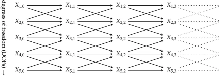
Figure 1.First time steps of a Bayesian network representing a multivariate dynamical system (or multivariate Markov chain){Xi}i∈V. Here we used V = J×T with J indicating spatial degrees of freedom and T the temporal extension. Then each node is indexed by a tuple(j,t)as shown. The shown edges are just an example, any two nodes within the same or subsequent columns can be connected as long as the target of the edge is not on the left of its origin.
Then we motivate briefly the use of specific and complete local integration (SLI and CLI) for an entity criterion on patterns. We then turn to more formal aspects of SLI and CLI. We first prove an upper bound for SLI and construct a candidate for a lower bound. We then go on to define the disintegration hierarchy and its refinement-free version. These structures are then used to prove the main result, thedisintegration theorem. This relates the SLI of a whole trajectories of a Bayesian network to the CLI of parts of these trajectories and vice versa.
3.1. Patterns
This section introduces the notion of patterns. These form the basic candidate structures for entities.
The structures we are trying to capture by entities should be analogous to spatially and temporally extended objects we encounter in everyday life (e.g. soap bubbles, living organisms). These objects seem to occur in the single history of the universe that also contains us. The purpose of patterns is then to capture arbitrary structures that occur within single trajectories or histories of a multivariate discrete dynamical system (see Fig. 1 for an example of a Bayesian network of such a system). Unlike entities, which we conceive of as special patterns that fulfil further criteria, patterns are formed by any combination of events at arbitrary times and positions. As an example we might think of a Game of Life cellular automaton. The time evolutions over multiple steps of the cells attributed to a glider or a block [see15, for a principled way to attribute cells to these] should be patterns but also arbitrary choices of subsets of cells (and their values) possibly extending over multiple timesteps together.
In the more general context of (finite) Bayesian networks there may be no interpretation of time or space. Nonetheless, we can define that a trajectory in this case fixes every random variable to a particular value. We then define patterns (and trajectories) formally in the following way.
Definition 3(Patterns and trajectories). Let{Xi}i∈V be set of random variables with index set V and state
spaces{Xi}i∈Vrespectively.
1. A pattern at A⊆V is an assignment
where xA ∈ XA. If there is no danger of confusion we also just write xAfor the pattern XA=xAat A.
2. Patterns XV =xVat V which fix the complete set{Xi}i∈Vof random variables are calledtrajectories.
3. A pattern xAis said to occur in trajectoryx¯V ∈ XVifx¯A =xA.
4. Each pattern xAuniquely defines a set of trajectoriesT(xA)via
T(xA) ={x¯V ∈ XV : ¯xA=xA}, (8)
i.e. the set of trajectories that xAoccurs in. Remarks:
• Note that for every xA ∈ XA we can form a pattern XA = xA so the set of all patterns is
S
A⊆VXA.
• Our notion of patterns is similar to “patterns” as defined in Ceccherini-Silberstein and Coornaert [31] and to “cylinders” as defined in Busicet al.[32]. However the notions there are explicitly restricted to single time-slices of (probabilistic) cellular automata. Our notion of patterns purposely lifts this restriction. Our notion is inspired by the usage of the term spatiotemporal pattern in Beer [153334] and we suggest that it formalises this notion.
The set of subsets ofXV defined by patterns and the set of all subsets 2XV (i.e. the power set) of
XV of a set of random variables{Xi}i∈Vare not equal. Formally:
[
B∈V
{T(xB)⊆ XV:xB∈ XB} 6=2XV. (9)
While patterns define subsets ofXV not every subset ofXVis defined (or captured) by a pattern. To see this we next show how to construct a subset ofXV that is not a pattern. First we define some extra terminology.
Definition 4. Let{Xi}i∈Vbe set of random variables with index set V and state spaces{Xi}i∈Vrespectively.
For a subsetD ⊆ XVthe setDAof all patterns at A that occur in one of the trajectories inDis defined as
DA:={xA∈ XA :∃x¯V ∈ XV, ¯xA =xA}. (10)
With this we get the following theorem which establishes the difference between the subsets of
XV captured by patterns and general subsets.
Theorem 1. Given a set of random variables{Xi}i∈V, a subsetD ∈ XV cannot be represented by a pattern
of{Xi}i∈V if and only if there exists A⊆V withDA ⊂ XA(proper subset) and|DA| >1, i.e. if neither all
patterns at A are possible nor a unique pattern at A is specified byD. Proof. See AppendixC.
3.2. Motivation of complete local integration as an entity criterion
We proposed to use patterns as the candidate structures for entities since patterns comprise arbitrary structures that occur within single trajectories of multivariate systems. Here we heuristically motivate our choice of using positive complete local integration as a criterion to select entities among patterns. In general such a criterion would give us, for any Bayesian network {Xi}i∈V a subset E({Xi}i∈V)⊆SA⊆VXAof the patterns.
same identity we also define entities by finding all parts that share identity with some given part. For the moment, let us decompose (as is often done8) the problem of identity into two parts
1. spatial identity and 2. temporal identity.
Our solution will make no distinction between these two aspects in the end. We note here that conceiving of entities (or objects) as composite of spatial and temporal parts as we do in this thesis is referred to as four-dimensionalism or perdurantism in philosophical discussions [see e.g. 35]. The opposing view holds that entities are spatial only and endure over time. This view is called endurantism. Here we will not go into the details of this discussion.
The main intuition behind complete local integration is that every part of an entity should make every other part more probable.
This seems to hold for example for the spatial identity of living organisms. Parts of living organisms rarely exist without the rest of the living organisms also existing. For example it is rare that an arm exists without a corresponding rest of a human body existing compared to an arm and the rest of a human body existing. The body (without arm) seems to make the existence of the arm more probable and vice versa. Similar relations between parts seem to hold for all living organisms but also for some non-living structures. The best example of a non-living structure we know of for which this is obvious are soap bubbles. Half soap bubbles (or thirds, quarters,...) only ever exist for split seconds whereas entire soap bubbles can persist for up to minutes. Any part of a soap bubble seems to make the existence of the rest more probable. Similarly, parts of hurricanes or tornadoes are rare. So what about spatial parts of structures that are not so entity-like? Does the existence of an arm make things more probable that are not parts of the corresponding body? For example does the arm make the existence of some piece of rock more probable? Maybe to a small degree as without the existence of any rocks in the universe humans are probably impossible. However, this effect is much smaller than the increase of probability of the existence of the rest of the body due to the arm.
These arguments concerned the spatial identity problem. However, for temporal identity similar arguments hold. The existence of a living organism at one point in time makes it more probable that there is a living organism (in the vicinity) at a subsequent (and preceding) point in time. If we look at structures that are not entity-like with respect to the temporal dimension we find a different situation. An arm at some instance of time does not make the existence of a rock at a subsequent instance much more probable. It does make the existence of a human body at a subsequent instance much more probable. So the human body at the second instance seems to be more like a future part of the arm than the rock. Switching now to patterns in sets of random variables we can easily formalise such intuitions. We required that for an entity every part of the structure, which is now a pattern xO, makes every other part more probable. A part of a pattern is a patternxbwithb ⊂O. If we require that every part of a pattern makes every other part more probable then we can write thatxOis an entity if:
min b⊂O
pO\b(xO\b|xb)
pO\b(xO\b)
>1. (11)
This is equivalent to
min b⊂O
pO(xO)
pO\b(xO\b)pb(xb)
>1. (12)
If we writeL2(O)for the set of all bipartitions ofOwe can rewrite this further as
min π∈L2(O)
pO(xO)
∏b∈πpb(xb)
>1. (13)
We can interpret this form as requiring that for every possible partitionπ ∈ L2(O)into two parts xb1,xb2 the probability of the whole patternxO = (xb1,xb2)is bigger than its probability would be if
the two parts were independent. To see this, note that if the two partsxb1,xb2 were independent we
would have
pO(xO) =:pb1,b2(xb1,xb2) =pb1(xb1)pb2(xb2). (14)
Which would give us
pO(xO)
∏b∈πpb(xb)
=1 (15)
for this partition.
From this point of view the choice of bipartitions only seems arbitrary. For example, the existence a partitionξinto three parts such that
pO(xO) =
∏
c∈ξpc(xc) (16)
seems to suggest that the patternxO is not an entity but instead composite of three parts. We can therefore generalise Eq. (13) to include all partitions L(O) (see Definition 2) ofO except the unit partition1O. Then we would say thatxOis an entity if
min π∈L(O)\1O
pO(xO)
∏b∈πpb(xb)
>1. (17)
This measure already results in the same entities as the measure we propose.
However, in order to connect with information theory, log-likelihoods, and related literature we formally introduce the logarithm into this equation.
Anticipating the definition of CLI in Definition8we then define theι-entities.
Definition 5(ι-entity). Given a multivariate Markov chain{Xi}i∈Va pattern xOis aι-entity if min
π∈L(O)\1O
miπ(xO)>0. (18)
Theι-entity-setEι({Xi}i∈V)is then defined as follows.
Definition 6(ci-entity-set). Given a multivariate Markov chain{Xi}i∈Vtheι-entity-set is the entity-set Eι({Xi}i∈V):={xO∈
[
A⊆V
XA:ι(xO)>0}. (19)
In the next sections we look at more formal properties of expressions that occur in these definitions.
3.3. Specific local integration
This section introduces the specific local integration (SLI). It also proves its upper bounds constructively and constructs an example of negative SLI.
3.3.1. General and deterministic case
Definition 7(Specific local integration (SLI)). Given a Bayesian network{X}i∈V and a pattern xO the
specific local integrationmiπ(xO)of xOwith respect to a partitionπof O⊆V is defined as
miπ(xO):=log
pO(xO)
∏b∈πpb(xb)
In this paper we use the convention thatlog00 :=0.
Theorem 2 (Deterministic specific local integration). Given a deterministic Bayesian network (DefinitionB.5), a uniform initial distribution over XV0(V0is the set of nodes without parents), and a pattern
xOwith O⊆V the SLI of xOwith respect to partitionπcan be expressed more specifically: Let N(xO)refer
to the number of trajectories in which xOoccurs. Then
miπ(xO) = (|π| −1)log|XV0| −log
∏b∈πN(xb)
N(xO)
. (21)
Proof. See AppendixB.2.
3.3.2. Upper bounds
In this section we present the upper bounds of SLI. These are of general interest, constructive proofs which may serve to familiarise the reader with the measure of SLI are given in AppendixD.
We first show constructively that if we can choose the Bayesian network and the pattern then SLI can be arbitrary large. This construction sets the probabilities of all blocks equal to the probability of the pattern. In the subsequent theorem we show that this property in general gives the upper bound of SLI if the cardinality of the partition is fixed. This leads directly tho the upper bound if the cardinality of the partition is not fixed in the next theorem. Finally we give the expressions of the bounds in the deterministic case for convenient reference.
Theorem 3(Upper bound of SLI). For any Bayesian network{X}i∈Vand pattern xOwith fixed pO(xO) =
q
1. The tight upper bound of the SLI with respect to any partitionπwith|π|=n fixed is max
{{Xi}i∈V:∃xO,pO(xO)=q} max
{π:|π|=n}miπ(xO)≤ −(n−1)logq. (22) 2. The upper bound is achieved if and only if for all b∈πwe have
pb(xb) =pO(xO) =q. (23)
3. The upper bound is achieved if and only if for all b∈πwe have that xOoccurs if and only if xboccurs. Proof. See AppendixD.1
Remarks:
• Note that this is the least upper bound for Bayesian networks in general. For a specific Bayesian network there might be no pattern that achieves this bound.
• The least upper bound of SLI increases with the improbability of the pattern and the number of parts that it is split into. IfpO(xO)→0 then we can have miπ(xO)→∞.
• Using this least upper bound it is easy to see the least upper bound for the SLI of a patternxO across all partitions|π|. We just have to note that|π| ≤ |O|.
3.3.3. Negative SLI
This section shows that SLI of a pattern xO with respect to partition π can be negative
Theorem 4. For any given probability q < 1and cardinality |π| = n > 1 of a partitionπ there exists a
pattern xOin a Bayesian network{Xi}i∈V such that q= pO(xO)and miπ(xO) =log
q
1−1−nqn
<0. (24)
Proof. See AppendixD.2
Remarks:
• The achieved value in Eq. (24) is also our best candidate for a greatest lower bound of SLI for givenpO(xO)and|π|. However, we have not been able to prove this yet.
• The construction equidistributes the probability 1−q(left to be distributed after the probability qof the whole pattern occurring is chosen) to the patterns ¯xO that arealmostthe same as the patternxO. These are almost the same in a precise sense: They differ in exactly one of the blocks ofπi.e. they differ by as little as can possibly be resolved/revealed by the partitionπ.
• An interpretation of the construction is that patterns which either occur as a whole or (with uniform probability) missing exactly one part always have negative SLI.
3.4. Complete local integration
We now define complete local integration (CLI) which forms the criterion distinguishing arbitrary patterns fromι-entities. SLI is defined with respect to a particular partition and a pattern
xA may have high SLI with respect to one partition but negative SLI with respect to another (see Section4). Therefore SLI seems to be ill suited to define entities since then the property of being an entity would depend on how we decide to split it into parts. In order to deal with this problem we follow Tononi and Sporns [12], Balduzzi and Tononi [13], Tononi [36] who have encountered similar problems with another measure of integration. The idea is to find the partition with respect to which the pattern is least integrated and use the SLI with respect to this as the value of CLI. In other words the CLI is the SLI ofxOwith respect to the partition thatdisintegrates xOthe most.
Definition 8((Complete) local integration). Given a Bayesian network{Xi}i∈V and a pattern xOof this
network the complete local integration ι(xO) of xO is the minimum SLI over the non-unit partitionsπ ∈ L(O)\1O:
ι(xO):= min
π∈L(O)\1O
miπ(xO). (25)
We call a pattern xOcompletely locally integrated ifι(xO)>0. Remarks:
• The reason for excluding the unit partition1OofL(O)(where1O={O}see Definition2) is that with respect to it every pattern has mi1O(xO) =0.
• Looking for a partition that minimises a measure of integration is known as the weakest link approach[37] to dealing with multiple partitions. We note here that this is not the only approach that is being discussed. Another approach is to look at weighted averages of all integrations. For a further discussion of this point in the case of the expected value of SLI see Ay [37] and references therein. An analysis of which approach is best suited for the local integration measure presented here is beyond the scope of this paper.
3.5. Disintegration
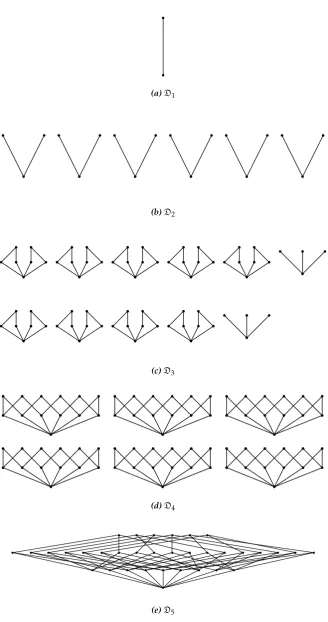
In this section we define the disintegration hierarchy and its refinement-free version. We then prove the disintegration theorem which is the main formal result of this paper. It exposes a connection between partitions minimising the SLI of a trajectory and the CLI of the blocks of such partitions. More precisely for a given trajectory the blocks of thefinestpartitions among those leading to a particular value of SLI consist only of completely locally integrated blocks. Conversely each completely locally integrated pattern is a block in such a finest partition leading to a particular value of SLI. The theorem therefore reveals the special role of patterns with positive CLI for the SLI of an entire trajectory of the system. For our purposes this theorem allows further interpretations of the measure of CLI which will be discussed in Section5.
Definition 9(Disintegration hierarchy). Given a Bayesian network{Xi}i∈Vand a trajectory xV ∈ XV, the
disintegration hierarchy of xVis the setD(xV) ={D1,D2,D3, ...}of sets of partitions of xVwith:
1.
D1(xV):=arg min
π∈L(V)
miπ(xV) (26)
2. and for i >1:
Di(xV):= arg min
π∈L(V)\D≺i(xV)
miπ(xV). (27)
whereD≺i(xV):=Sj<iDj(xV). We callDi(xV)the i-th disintegration level. Remark:
• Note that arg min returns all partitions that achieve the minimum SLI if there is more than one. • Since the Bayesian networks we use are finite, the partition lattice L(V) is finite, the set of
attained SLI values is finite, and the number|D|of disintegration levels is finite.
• In most cases the Bayesian network contains some symmetries among their mechanisms which cause multiple partitions to attain the same SLI value.
• For each trajectoryxVthe disintegration hierarchyDthen partitions the elements ofL(V)into subsetsDi(xV)of equal SLI. The levels of the hierarchy have increasing SLI.
Definition 10. LetL(V)be the lattice of partitions of set V and letEbe a subset ofL(V). Then for every elementπ∈L(V)we can define the set
ECπ:={ξ∈E:ξCπ}. (28)
That isECπis the set of partitions inEthat are refinements ofπ.
Definition 11 (Refinement-free disintegration hierarchy). Given a Bayesian network {Xi}i∈V, a
trajectory xV ∈ XV, and its disintegration hierarchyD(xV)the refinement-free disintegration hierarchy of
xVis the setDJ(xV) ={DJ1,DJ2,DJ3, ...}of sets of partitions of xVwith:
1.
DJ1(xV):={π∈D1(xV):D1(xV)Cπ=∅}, (29) 2. and for i >1:
DJi (xV):={π∈Di(xV):D≺i(xV)Cπ=∅} (30) Remark:
partition that occurs in the refinement-free disintegration hierarchy at thei-th level is a finest partition that achieves such a low level of SLI or such a high level of disintegration.
• As we will see below, the blocks of the partitions in the refinement-free disintegration hierarchy are the main reason for defining the refinement-free disintegration hierarchy.
Theorem 5(Disintegration theorem). Let{Xi}i∈Vbe a Bayesian network, xV ∈ XV one of its trajectories,
andDJ(xV)the associated refinement-free disintegration hierarchy.
1. Then for everyDJi (xV) ∈DJ(xV)we find for every b ∈ πwithπ ∈ DJi (xV)that there are only the
following possibilities:
(a) b is a singleton, i.e. b={i}for some i∈V, or (b) xbis completely locally integrated, i.e.ι(xb)>0.
2. Conversely, for any completely locally integrated pattern xA, there is a partitionπA∈L(V)and a level DJ
iA(xV)∈DJ(xV)such that A∈πAandπA ∈DJiA(xV).
Proof. ad1 We prove the theorem by contradiction. For this assume that there is blockbin a partition π∈DJi (xV)which is neither a singleton nor completely integrated. Letπ∈DJi (xV)andb∈π. Assumebis not a singleton i.e. there existi6=j∈Vsuch thati∈bandj∈b. Also assume thatb is not completely integrated i.e. there exists a partitionξofbwithξ6=1bsuch that miξ(xb)≤0. Note that a singleton cannot be completely locally integrated as it does not allow for a non-unit partition. So together the two assumptions implypb(xb)≤∏d∈ξpd(xd)with|ξ|>1. But then
miπ(xV) =log
pV(xV)
pb(xb)∏c∈π\bpc(xc) (31)
≥log pV(xV)
∏d∈ξpd(xd)∏c∈π\bpc(xc)
(32)
We treat the cases of “>” and “=” separately. First, let
miπ(xV) =log
pV(xV)
∏d∈ξpd(xd)∏c∈π\bpc(xc)
. (33)
Then we can defineρ:= (π\b)∪ξsuch that
1. miρ(xV) =miπ(xV)which implies thatρ∈Di(xV)becauseπ∈Di(xV), and 2. ρCπwhich contradictsπ ∈DJi (xV).
Second, let
miπ(xV)>log
pV(xV)
∏d∈ξpd(xd)∏c∈π\bpc(xc). (34) Then we can defineρ:= (π\b)∪ξsuch that
miρ(xV)<miπ(xV), (35) which contradicts miπ(xV)∈DJi (xV).
ad2 LetπA :={A} ∪ {{j}}j∈V\A. SinceπAis a partition ofVit is an element of some disintegration level DiA. Then partition πA is also an element of the refinement-free disintegration level DJ
letξ∈L(V),ξ 6=πAandξ CπAsinceπAonly contains singletons apart fromAthe partition ξmust split the blockAinto multiple blocksc∈ξ|A. Sinceι(xA)>0 we know that
miξ|A(xA) =log pA
(xA)
∏c∈ξ|A pc(xc)
>0 (36)
so that∏c∈ξ|Apc(xc)< pA(xA)and
miξ(xV) =log
pV(xV)
∏c∈ξ|Apc(xc)∏i∈V\Api(xi)
(37)
>log pV(xV) pA(xA)∏i∈V\Api(xi)
(38)
=miπA(xV). (39) Thereforeξis on a disintegration levelDk(xV)withk> iA, but this is true for any refinement ofπAsoD≺iA(xV)CπA =∅andπ
A∈DJ
iA(xV).
4. Examples
In this section we investigate the structure of integrated and completely locally integrated spatiotemporal patterns as it is revealed by the disintegration hierarchy. First we take a quick look at the trivial case of a set of independent random variables. Then we look at two very simple multivariate Markov chains. We use the disintegration theorem (Theorem5) to extract the completely locally integrated spatiotemporal patterns.
4.1. Set of independent random variables
Let us first look at a set{Xi}i∈V of independently and identically distributed random variables. For each trajectoryxV ∈ XVwe can then calculate SLI with respect to a partitionπ∈L(V). For every
A⊆Vand everyxA ∈ XAwe havepA(xA) =∏i∈Api(xi). Then we find for everyπ∈L(V):
miπ(xV) =0. (40)
This shows that the disintegration hierarchy for eachxV ∈ XV contains only a single disintegration levelD(xV) = {D1}withD1 =L(V). The finest partition ofL(V)is its zero element0which then constitutes the only element of the refinement-free disintegration levelDJ1 ={0}. Recall that the zero element of a partition lattice only consists of singleton sets as blocks. The set of completely locally integrated patterns i.e. the set ofι-entities in a given trajectoryxVis then the set{xi:i∈V}.
Next we will look at more structured systems.
4.2. Two constant and independent binary random variables: MC=
4.2.1. Definition
Define the time- and space-homogeneous multivariate Markov chain MC= with Bayesian network{Xj,t}j∈{1,2},t∈{0,1,2}and
•
pa(j,t) =
(
∅ ift=0,
{(j,t−1)} else, (41)
•
pj,t(xj,t|xj,t−1) =δxj,t−1(xj,t) = (
1 ifxj,t=xj,t−1,
X1,1 X1,2 X1,3
X2,1 X2,2 X2,3
Figure 2.Bayesian network of MC=. There is no interaction between the two processes.
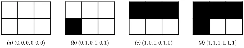
(a)(0, 0, 0, 0, 0, 0) (b)(0, 1, 0, 1, 0, 1) (c)(1, 0, 1, 0, 1, 0) (d)(1, 1, 1, 1, 1, 1)
Figure 3.Visualisation of the four possible trajectories of MC=. In each trajectory the time index increases from left to right. There are two rows corresponding to the two random variables at each time step and three columns corresponding to the three time-steps we are considering here.
•
pj,0(xj,0) =1/4. (43)
The Bayesian network can be seen in Fig.2.
4.2.2. Trajectories
In order to get the disintegration hierarchyD(xV)we have to choose a trajectoryxVand calculate the SLI of each partitionπ ∈ L(V). There are only four different trajectories possible inMC= and they are:
xV= (x1,0,x2,0,x1,1,x2,1,x1,2,x2,2) =
(0, 0, 0, 0, 0, 0) ifx1,0=0,x2,0=0;
(0, 1, 0, 1, 0, 1) ifx1,0=0,x2,0=1;
(1, 0, 1, 0, 1, 0) ifx1,0=1,x2,0=0;
(1, 1, 1, 1, 1, 1) ifx1,0=1,x2,0=1.
(44)
Each of these trajectories has probabilitypV(xV) = 1/4 and all other trajectories havepV(xV) = 0. We call the four trajectories thepossible trajectories. We visualise the possible trajectories as a grid with each cell corresponding to one variable. The spatial indices are constant across rows and time-slices Vtcorrespond to the columns. A white cell indicates a 0 and a black cell indicates a 1. This results in the grids of Fig.3.
4.2.3. Partitions of trajectories
The disintegration hierarchy is composed out of all partitions in the lattice of partitionsL(V). Recall that we are partitioning the entire spatially and temporally extended index set V of the Bayesian network and not only the time-slices. Blocks in the partitions ofL(V)are then, in general, spatiotemporally and not only spatially extended patterns.
0 50 100 150 200 0
1 2 3 4
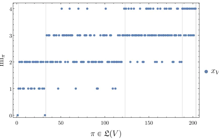
Figure 4. Specific local integrationsmiπ(xV)of any of the four trajectories xVseen in Fig.3with respect to allπ∈L(V). The partitions are ordered according to an enumeration with increasing cardinality|π|(see38,
chap. 4.3.3 for the method). We indicate with vertical lines at what partitions the cardinality|π|increases by
one.
partition). The number of partitions of a set of cardinality|V|into|π|blocks is the Stirling number
S(|V|,|π|). For|V|=6 we find the Stirling numbers:
|π| 1 2 3 4 5 6
S(|V|,|π|) 1 31 90 65 15 1 (45)
It is important to note that the partition lattice L(V) is the same for all trajectories as it is composed out of partitions ofV. On the other hand the values of SLI miπ(xV) with respect to the partitions inL(V)generally depend on the trajectoryxV.
4.2.4. SLI values of the partitions
We can calculate the SLI miπ(xV)of every trajectoryxV with respect to each partitionπ∈L(V) according to Definition7:
miπ(xV):=log pV
(xV)
∏b∈πpb(xb)
. (46)
In the case ofMC=the SLI values with respect to each partition do not depend on the trajectories. For an overview we plotted the values of SLI with respect to each partitionπ ∈ L(V)for any trajectory ofMC=in Fig.4. We can see in Fig.4that the cardinality does not determine the value of SLI. At the same time there seems to be a trend to higher values of SLI with increasing cardinality of the partition. We can also observe that only five different values of SLI are attained by partitions on this trajectory. We will collect these classes of partitions with equal SLI values in the disintegration hierarchy next.
4.2.5. Disintegration hierarchy
0 50 100 150 200 0
1 2 3 4
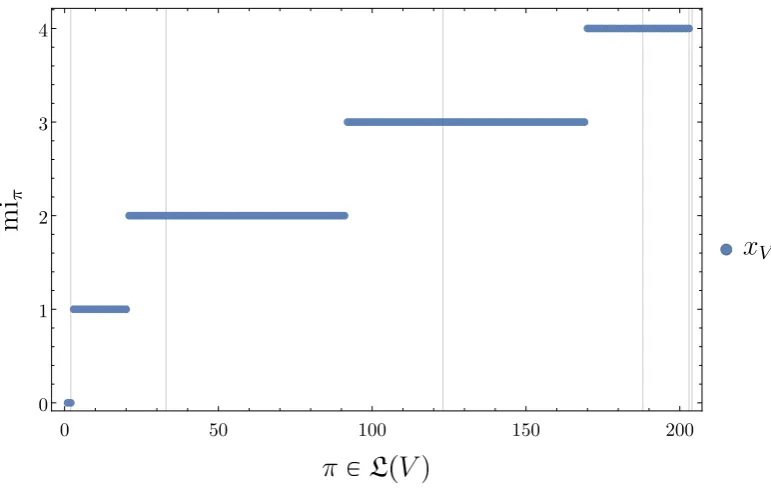
Figure 5.Same as Fig.4but with the partitions sorted according to increasing SLI.
the disintegration levels Di(xV) partially ordered by refinement. If we sort the partitions of any trajectory of MC= according to increasing SLI value we obtain Fig. 5. There we see groups of partitions attaining the SLI values{0, 1, 2, 3, 4}(precisely) these groups are the disintegration levels
{D1(xV),D2(xV),D3(xV),D4(xV),D5(xV)}. The exact numbers of partitions in each of the levels are:
i 1 2 3 4 5
miπ 0 1 2 3 4
|Di| 2 18 71 78 34
(47)
Next we look at the Hasse diagram of each of those disintegration levels (partially ordered by refinement). Since the disintegration levels are subsets of the partition latticeL(V), they are in general not lattices by themselves. The Hasse diagrams visualise the set of partitions in each disintegration level partially ordered by refinementC. Recall that in Hasse diagrams of such posets the partitions are arranged such that ifπ 6= ξandπ C ξthenπ is drawn belowξ. Also, an edge is drawn from partitionπtoξif onecoversthe other e.g. ifπ C:ξ(note the colon indicating the covering relation). The Hasse diagrams are shown in Fig.6. We see immediately that within each disintegration level apart from the first and the last the Hasse diagrams contain multiple connected components.
Furthermore, within a disintegration level the connected components often have the same Hasse diagrams. For example in D2 (Fig. 6b) we find six connected components with three partitions each. The identical refinement structure of the connected components is related to the symmetries of the probability distribution over the trajectories. As it requires further notational overhead and is straightforward we do not describe these symmetry properties formally. In order to see the symmetries, however, we visualise the partitions themselves in the Hasse diagrams in Fig.7.
(a)D1
(b)D2
(c)D3
(d)D4
(e)D5
Figure 7.Hasse diagram ofD2of MC=trajectories. Here we visualise the partitions at each vertex. The blocks of a partition are the cells of equal colour. Note that we can obtain all six disconnected components from one by symmetry operations that are respected by the joint probability distribution pV. For example we can shift each row individually to the left or right since every value is constant in each row. We can also switch top and bottom row since they have the same probability distributions even if1and0are exchanged.
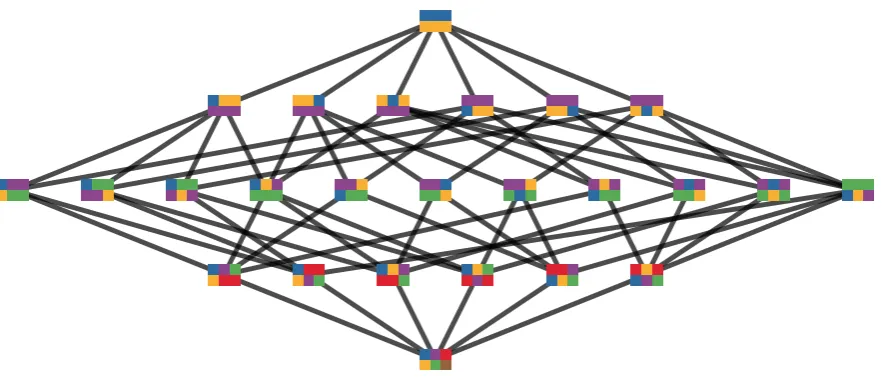
Figure 8. Hasse diagrams of the refinement-free disintegration hierarchyDJ of MC= trajectories. Here we visualise the partitions at each vertex. The blocks of a partition are the cells of equal colour. It turns out that partitions that are on the same horizontal level in this diagram correspond exactly to a level in the refinement-free disintegration hierarchyDJ. The i-th horizontal level starting from the top corresponds toDJi . Take for example the second horizontal level from the top. The partitions on this level are just the minimal elements of the poset
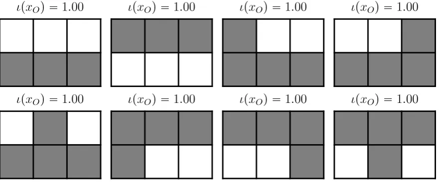
Figure 9.All distinct completely integrated composite patterns (singletons are not shown) on the first possible trajectory of MC=. The value of complete local integration is indicated above each pattern. We display patterns by colouring the cells corresponding to random variables that are not fixed to any value by the pattern in grey. Cells corresponding to random variables that are fixed by the pattern are coloured according to the value i.e. white for0and black for1.
4.2.6. Completely integrated patterns
Having looked at the disintegration hierarchy we now make use of it by extracting the completely (locally9) integrated patterns of the four trajectories of MC=. Recall that due to the disintegration theorem (Theorem 5) we know that all blocks in partitions that occur in the refinement-free disintegration hierarchy are either singletons or correspond to completely integrated patterns. If we look at the refinement-free disintegration hierarchy in Fig.8we see that many blocks occur in multiple partitions and across disintegration levels. We also see that there are multiple blocks that are singletons. If we ignore singletons, which are trivially integrated as they cannot be partitioned, we end up with eight different blocks. Since the disintegration hierarchy is the same for all four possible trajectories these blocks are also the same for each of them (note that this is the case for MC= but not in general as we will see in Section 4.3). However, the patterns that result are different due to the different values within the blocks. We show the eight completely integrated patterns and their complete local integration (Definition8) on the first trajectory in Fig.9and on the second trajectory in Fig.10.
Since the disintegration hierarchies are the same for the four possible trajectories of MC= we get the same refinement-free partitions and therefore the same blocks containing the completely integrated patterns. This is apparent when comparing Figs.9and 10and noting that each pattern occurring on the first trajectory has a corresponding pattern on the second trajectory that differs (if at all) only in the values of the cells it fixes and not in what values it fixes. More visually speaking, for each pattern in Fig.9there is a corresponding pattern in Fig.10leaving the same cells grey.
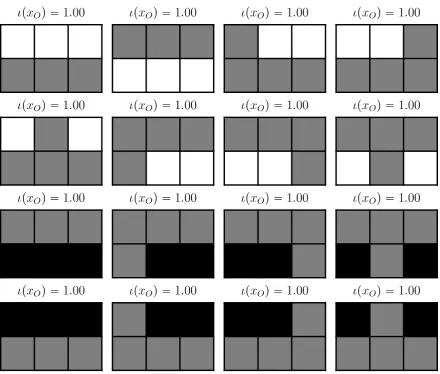
If we are not interested in a particular trajectory we can also look at all different completely integrated patterns on any trajectory. ForMC=these are shown in Fig.11We see that all completely integrated patterns xO have the same value of complete local integration ι(xO) = 1. This can be explained using the deterministic expression for the SLI of Eq. (21) and noting that for MC= if any of the values xj,t is fixed by a pattern then (xj,s)s∈T = xj,T are determined since they must be the
Figure 10.All distinct completely integrated composite patterns on the second possible trajectory of MC=. The value of complete local integration is indicated above each pattern.
same value. This means that the number of trajectoriesN(xj,S)in which any patternxj,SwithS⊆T occurs is eitherN(xj,S) =0, if the pattern is impossible, orN(xj,S) =2 since there are two trajectories compatible with it. Note that all blocksxbin any of the completely integrated pattern and all pattern
xOthemselves are of the formxj,S withS ⊆ T. Let N(xj,S) =: Nand plug this into Eq. (21) for an arbitrary partitionπ:
miπ(xO) = (|π| −1)log|XV0| −log
∏b∈πN(xb)
N(xO) (48)
= (|π| −1)log|XV0| −log
N|π|
N (49)
= (|π| −1)log
|XV0|
N . (50)
To get the complete local integration value we have to minimise this with respect toπwhere|π| ≥2. So for|XV0|=4 andN=2 we getι(xO) =1.
Another observation is that the completely integrated patterns are all limited to one of the two rows. This shows on a simple example that, as we would expect, completely integrated patterns cannot extend from one independent process to another.
4.3. Two random variables with small interactions
In this section we look at a system almost identical to that of Section4.2but with a kind of noise introduced. This allows all trajectories to occur and is designed to test whether the spatiotemporal patterns maintain integration in the face of noise.
4.3.1. Definition
We define the time- and space-homogeneous multivariate Markov chain MCe via the Markov matrixPwith entries
Pf(x1,t+1,x2,t+1),f(x1,t,x2,t)=pJ,t+1(x1,t+1,x2,t+1|x1,t,x2,t) (51) where we define the function f :{0, 1}2→[1 : 4]via
f(0, 0) =1,f(0, 1) =2,f(1, 0) =3,f(1, 1) =4. (52) With this conventionPis
P=
1−3e e e e
e 1−3e e e
e e 1−3e e
e e e 1−3e
(53)
This means that the state of bothrandom variables remains the same with probability 1−3e and transitions into each of the other possible combinations with probabilitye. In the following we set e=1/100. The initial distribution is again the uniform distribution
pj,0(xj,0) =1/4. (54)
X1,1 X1,2 X1,3
X2,1 X2,2 X2,3
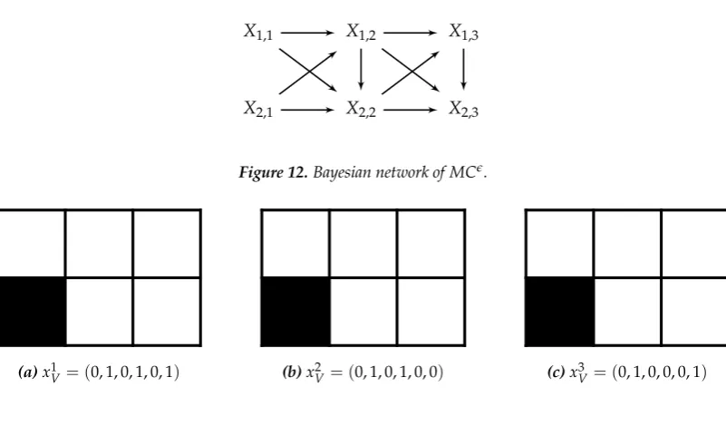
Figure 12.Bayesian network of MCe.
(a)x1
V= (0, 1, 0, 1, 0, 1) (b)x2V= (0, 1, 0, 1, 0, 0) (c)xV3 = (0, 1, 0, 0, 0, 1)
Figure 13. Visualisation of three trajectories of MCe. In each trajectory the time index increases from left to right. There are two rows corresponding to the two random variables at each time step and three columns corresponding to the three time-steps we are considering here. We can see that the first trajectory (ina) makes noe-transitions, the second (inb) makes one from t=2to t=1, and the third (inc) makes two.
4.3.2. Trajectories
In this system all trajectories are possible trajectories. This means there are 26 = 64 possible trajectories, since every one of the six random variables can be in any of its two states. There are three classes of trajectories with equal probability of occurring. The first class with the highest probability of occurring are the four possible trajectories ofMC=. Then there are 24 trajectories that make a single e-transition (i.e. a transition where the next pair is not the same as the current one(x1,t+1,x2,t+1)6=
(x1,t,x2,t), these transitions occur with probabilitye), and 36 trajectories with twoe-transitions. We pick only one trajectory from each class. The representative trajectories are shown in Fig.13 and will be denoted x1V,x2V, and x3V respectively. The probabilities are pV(x1V) = 0.235225,pV(x2V) = 0.0024250,pV(x3V) =0.000025.
4.3.3. SLI values of the partitions
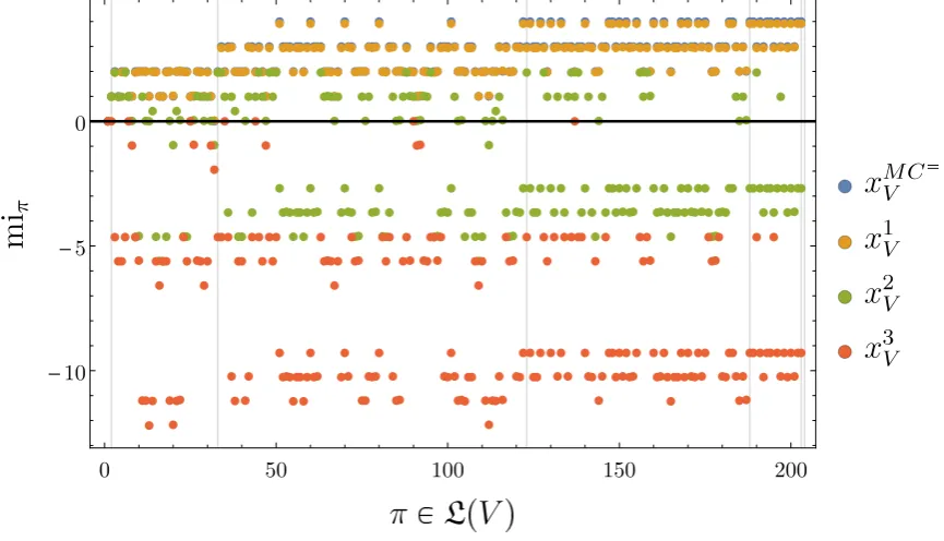
Again we calculate the SLI miπ(xV) of every trajectory xV with respect to each partition π ∈ L(V). In contrast to MC= the SLI values with respect to each partition of MCe do depend on the trajectories. We plot the values of SLI with respect to each partitionπ ∈ L(V)for the three representative trajectories in Fig.14.
It turns out that the SLI values ofx1V are almost the same as those of MC= in Fig.4with small deviations due to the noise. This should be expected asx1Vis also a possible trajectory ofMC=. Also note that trajectoriesx2V,x3V exhibit negative SLI with respect to some partitions. In particular, x3V has non-positive SLI values with respect to any partition. This is due to the low probability of this trajectory compared to its parts. The blocks of any partition have so much higher probability than the entire trajectory that the product of their probabilities is still greater or equal to the trajectory probability.
4.3.4. Completely integrated patterns
In this section we look at the completely integrated patterns for each of the three representative trajectoriesxk
0 50 100 150 200 -10
-5 0
Figure 14. Specific local integrationsmiπ(xV)of one of the four trajectories of MC= (measured w.r.t. the probability distribution of MC=), here denoted xVMC= (this is the same data as in Fig. 4), and the three representative trajectories xk
V,x ∈ {1, 2, 3}of MCe (measured w.r.t. the probability distribution of MCe) seen in Fig.13with respect to allπ∈L(V). The partitions are ordered as in Fig.4with increasing cardinality
|π|. Vertical lines indicate partitions where the cardinality|π|increases by one. Note that the values of xVMC=
Figure 15.All distinct completely integrated composite patterns on the first trajectory x1
Figure 16.All distinct completely integrated composite patterns on the second trajectory x2Vof MCe. The value of complete local integration is indicated above each pattern.
Figure 17.All distinct completely integrated composite patterns on the third trajectory x3Vof MCe. The value of complete local integration is indicated above each pattern.
in Figs.15to17. In contrast to the situation of MC= we now have completely integrated patterns with varying values of complete local integration.
On the first trajectoryx1V we find all the eight patterns that are completely locally integrated in MC=(see Fig.10). These are also more than an order of magnitude more integrated than the rest of the completely integrated patterns. This is also true for the other two trajectories.
5. Discussion
the present state of the computational models and, without approximations, this was out of reach computationally. We will discuss this further below.
In Section 3.3 we defined SLI and gave its expression for deterministic Bayesian networks (including cellular automata) as well. We also established the least upper bound of SLI with respect to a partitionπ of cardinalityn for a pattern xA with probabilityq. This upper bound is achieved if each of the blocks xb in the partition π occur if and only if the whole pattern xO occurs. This is compatible with our interpretation of entities since in this case clearly the occurrence of any part of the pattern leads necessarily to the occurrence of the entire pattern (and not only vice versa).
We also presented a candidate for a greatest lower bound of SLI with respect to a partition of cardinalitynfor a pattern with probabilityq. Whether this is the greatest lower bound or not it shows a case for which SLI is always negative. This happens if either the whole patternxA occurs (with probabilityq) or one of the “almost equal” patterns occurs, each with identical probability. A pattern yAis almost equal toxAwith respect toπin this sense if it only differs at one of the blocksb∈ πi.e. ifyA = (xA\b,zb)wherezb6=xb. This construction makes as many parts as possible (i.e. all but one) occur as many times as possible without the whole pattern occurring. This creates large marginalised probabilities pb(xb) for each part/block which means that their product probability also becomes large.
Beyond these quantitative interpretations an interpretation of the greatest lower bound candidate seems difficult. A more intuitive candidate for the opposite of an integrated pattern seem to be patterns with independent parts i.e. zero SLI but quantitatively these are not on the opposite end of the SLI spectrum. A more satisfying interpretation of the presented candidate is still to be found.
In Section4we investigated SLI and CLI in three simple example sets of random variables. We found that if the random variables are all independently distributed the according entities are just all the possiblexj ∈ Xjof each of the random variables Xj ∈ {Xi}i∈V. This is what we would expect from an entity criterion. There are no entities with any further extent than a single random variable and each value corresponds to a different entity.
For the simple Markov chain MC= composed out of two independent and constant processes we presented the entire disintegration hierarchy and the Hasse diagrams of each disintegration level ordered by refinement. The Hasse diagrams reflected the highly symmetric dynamics of the Markov chain via multiple identical components. We also calculated the completely locally integrated patterns i.e. theι-entities ofMC=.
These included the expected three timestep constant patterns within each of the two independent processes. It also included the two timestep parts of these constant patterns. This may be less expected. It shows that parts of completely integrated patterns can be completely integrated patterns themselves. We note that these “sub-entities (those that are parts of larger entities) are always on a different disintegration level than their “super-entities (the larger entities). We can speculate that the existence of such sub- and super-entities on different disintegration levels may find an interpretation through multicellular organisms or similar structures. However, the overly simplistic examples here only serve as basic models for the potential phenomena, but are still far to simplistic to warrant any concrete interpretation in this direction.