University of Pennsylvania
ScholarlyCommons
Publicly Accessible Penn Dissertations
Summer 8-12-2011
A New Dynamic Duration Model
Fei Chen
University of Pennsylvania, [email protected]
Follow this and additional works at:http://repository.upenn.edu/edissertations Part of theEconometrics Commons
This paper is posted at ScholarlyCommons.http://repository.upenn.edu/edissertations/401
For more information, please [email protected].
Recommended Citation
Chen, Fei, "A New Dynamic Duration Model" (2011).Publicly Accessible Penn Dissertations. 401.
A New Dynamic Duration Model
Abstract
In this dissertation, I propose a new model for the analysis of financial durations. The new model improves upon several limitations of the autoregressive conditional duration (ACD) model considered in Engle and Russell (Econometrica 66(5) (1998) 1127-1162). Instead of adopting the multiplicative error form assumed by the ACD model, I establish a mixture of exponentials representation for durations from general point process theory. Based on the representation, I develop the Markov switching multifractal duration (MSMD) model. I present the geometric ergodicity property of MSMD and show that the MSMD can explain most stylized facts of financial durations, especially the long memory feature. An extensive empirical study shows MSMD compares favorably with ACD both in- and out-of-sample. For long horizon forecasting, MSMD dominates ACD, which confirms that MSMD can explain long range dependence in durations.
Degree Type Dissertation
Degree Name
Doctor of Philosophy (PhD)
Graduate Group Economics
First Advisor Francis X. Diebold
Second Advisor Frank Schorfheide
Third Advisor Kyungchul Song
Keywords
multifractal, duration
A NEW DYNAMIC DURATION MODEL
Fei Chen
A DISSERTATION
in
Economics
Presented to the Faculties of the University of Pennsylvania in Partial
Fulfillment of the Requirements for the Degree of Doctor of Philosophy
2011
Francis X. Diebold, Professor of Economics Supervisor of Dissertation
Dirk Krueger, Professor of Economics Graduate Group Chairperson
Dissertation Committee
Frank Schorfheide, Professor of Economics
A NEW DYNAMIC DURATION MODEL
COPYRIGHT
2011
Acknowledgements
First and foremost, I am indebted to my adviser Frank Diebold for his guidance and
support. He first introduced me to the multifractal volatility models, and opened
the door of multifractal processes for me. He has patiently mentored me through
the last few years of my Ph.D. journey.
I am also very grateful to my my committee members, Frank Schorfheide and
Kyungchul Song, for their encouragement, and valuable suggestions.
I thank all my friends at the University of Pennsylvania, who have made all the
difference. I especially thank Clare Wang, who has made this journey wonderful.
Lastly and most importantly, I would like to thank my parents Dezhen Chen and
ABSTRACT
A NEW DYNAMIC DURATION MODEL
Fei Chen
Francis X. Diebold
In this dissertation, I propose a new model for the analysis of financial durations.
The new model improves upon several limitations of the autoregressive conditional
duration (ACD) model considered in Engle and Russell (Econometrica 66(5) (1998)
1127-1162). Instead of adopting the multiplicative error form assumed by the ACD
model, I establish a mixture of exponentials representation for durations from general
point process theory. Based on the representation, I develop the Markov switching
multifractal duration (MSMD) model. I present the geometric ergodicity property
of MSMD and show that the MSMD can explain most stylized facts of financial
durations, especially the long memory feature. An extensive empirical study shows
MSMD compares favorably with ACD both in- and out-of-sample. For long horizon
forecasting, MSMD dominates ACD, which confirms that MSMD can explain long
Contents
Acknowledgements iii
1 Introduction 1
2 Point Processes and Mixture of Exponentials Representation 6
2.1 Notation and Definition . . . 6
2.2 Random Change of Time . . . 8
2.3 Mixture of Exponentials Representation . . . 9
3 Markov Switching Multifractal Duration 11 4 Model Properties 14 4.1 Geometric Ergodicity . . . 14
4.2 Clustering Effect . . . 15
4.3 Nonlinearity . . . 16
4.4 Overdispersion . . . 16
4.5 Long Memory Feature . . . 16
4.6 Discussion . . . 18
5 Empirical Studies 20 5.1 Data Description . . . 21
5.2 Daily Seasonality . . . 22
5.4 Estimation Method . . . 23
5.5 Model Diagnostics . . . 23
5.6 Estimation Results . . . 24
5.6.1 Overdispersion Test . . . 24
5.6.2 Comparison with ACD . . . 25
List of Tables
1 Twenty Stocks: Symbol and Company Name . . . 29
2 Basic Statistics: Low Trading Group . . . 30
3 Basic Statistics: High Trading Group . . . 31
4 Model Estimation: AA . . . 32
5 ACD Model Estimation: AA . . . 33
6 Model Estimation: ABT . . . 34
7 ACD Model Estimation: ABT . . . 35
8 Model Estimation: AXP . . . 36
9 ACD Model Estimation: AXP . . . 37
10 Model Estimation: BAC . . . 38
11 ACD Model Estimation: BAC . . . 39
12 Model Estimation: CSCO . . . 40
13 ACD Model Estimation: CSCO . . . 41
14 Model Estimation: DELL . . . 42
15 ACD Model Estimation: DELL . . . 43
16 Model Estimation: DOW . . . 44
17 ACD Model Estimation: DOW . . . 45
18 Model Estimation: F . . . 46
19 ACD Model Estimation: F . . . 47
20 Model Estimation: GE . . . 48
22 Model Estimation: IBM . . . 50
23 ACD Model Estimation: IBM . . . 51
24 Model Estimation: INTC . . . 52
25 ACD Model Estimation: INTC . . . 53
26 Model Estimation: JNJ . . . 54
27 ACD Model Estimation: JNJ . . . 55
28 Model Estimation: KO . . . 56
29 ACD Model Estimation: KO . . . 57
30 Model Estimation: MCD . . . 58
31 ACD Model Estimation: MCD . . . 59
32 Model Estimation: MRK . . . 60
33 ACD Model Estimation: MRK . . . 61
34 Model Estimation: MSFT . . . 62
35 ACD Model Estimation: MSFT . . . 63
36 Model Estimation: TXN . . . 64
37 ACD Model Estimation: TXN . . . 65
38 Model Estimation: WFC . . . 66
39 ACD Model Estimation: WFC . . . 67
40 Model Estimation: WMT . . . 68
41 ACD Model Estimation: WMT . . . 69
42 Model Estimation: XRX . . . 70
43 ACD Model Estimation: XRX . . . 71
44 Overdispersion Test Statistics Comparison . . . 72
45 Model Comparison: in Sample Fit . . . 73
46 Model Comparison: BIC . . . 74
47 Model Comparison: out of Sample Forecast . . . 75
48 Model Comparison: in Sample Fit . . . 76
List of Figures
1 An Example of Duration Dynamics . . . 79
2 Clustering Effect at Different Time Scale . . . 80
Chapter 1
Introduction
The last two decades have witnessed a growing interest in theoretical and empirical
modeling of the ultimate high-frequency financial data. A salient feature of these
intra-day tick-by-tick data is that transactions are irregularly spaced in time.
Many empirical studies take these irregular durations as exogenous sampling
schemes and tend to aggregate the data to fixed intervals in accordance with the usual
low-frequency data such as daily, weekly, monthly data. Such temporal aggregation
facilitates empirical analysis, but also causes two problems. First, the aggregation
will lose information and introduce unknown bias from a statistical view. A¨ıt-Sahalia
and Mykland (2003) discusses the effects of sampling randomness and discreteness
when estimating continuous time processes. Second, there is little theory guidance
on how to choose length of the fixed interval. Bandi and Russell (2008) discusses
how to choose the optimal sampling interval when estimating realized volatilities.
More importantly, the irregular duration is an endogenous variable, which has
economic information content. It reflects the speed of information flow on the
finan-cial market, see, e.g., Hasbrouck (1999). Easley and O’Hara (1992) gives a market
microstructure interpretation of intertrade durations. The theoretical model suggests
the dynamics of durations should have clustering effect, i.e., short (long) durations
actual data. Figure 1 gives one example. From the figure, one can see the durations
not only have clustering effect, but also have substantial outliers.
In this dissertation, I propose a new model, the Markov switching multifractal
du-ration (MSMD) model, to analyze these irregular dudu-rations. The MSMD model can
explain most stylized facts of intertrade durations found in empirical studies:
clus-tering effect; overdispersion1, the standard deviation being greater than the mean; long memory, autocorrelations decreasing hyperbolically; strong nonlinearities in the
dynamics. Furthermore the MSMD model predicts there should be clustering effect
at all time scales, and this feature is found in real data.
The first econometric model to explore the information content of intertrade
du-rations is the Autoregressive Conditional Duration (ACD) model proposed by Engle
and Russell (1998). The basic ACD model assumes a multiplicative error form, where
duration is the product of conditional mean and error2. Such a specification has two
components: the dynamics of the mean and the distribution of the error. Engle and
Russell assume a GARCH-type dynamics with iid exponential or iid Weibull errors.
The specification of the basic ACD model is too restrictive. The GARCH-type
dynamics can explain the clustering effect in durations, but can hardly capture other
stylized facts. For example, the standardized durations of the basic ACD model with
exponential error should have equal dispersion, but in practice, they still show excess
dispersion.
Numerous extensions of the basic ACD models have been developed in the
liter-ature. Those include the logarithmic ACD model of Bauwens and Giot (2000), the
Box-Cox and exponential ACD models of Dufour and Engle (2000), the threshold
ACD model of Zhang et al. (2001), the Stochastic Conditional Duration (SCD)
mod-el of Bauwens and Veredas (2004), the stochastic volatility duration (SVD) modmod-el
of Ghysels et al. (2004), the smooth transition ACD model of Meitz and Ter¨asvirta
1Giot (2000) reports that some volume duration series (durations for volume to reach some
threshold) can exhibit underdispersion. All durations between transactions and price changes (quote changes) show overdispersion. In this paper, I don’t consider volume durations.
(2006), the augmented ACD model of Fernandes and Grammig (2006), the
fraction-ally integrated ACD model of Jasiak (1999) and the long memory stochastic duration
model of Deo et al. (2010). None of these extensions can explain both nonlinearity
and long memory at the same time; while the MSMD model can explain nonlinearity
and long memory in one model.
One strand of the extensions is to use more flexible functional forms for the error
distribution, see Lunde (1999), Grammig and Maurer (2000), De Luca and Zuccolotto
(2003), De Luca and Gallo (2004), Drost and Werker (2004), Hujer and Vuletic
(2007), Sun et al. (2008), De Luca and Gallo (2009). The distributions being used
are Gamma distribution, generalized Gamma distribution, Burr distribution, mixed
exponential distribution, etc. On the one hand, these distributions are very flexible
for all practical purposes. On the other hand, the choice of a particular distribution
is arbitrary, and is mostly based on convenience and analytical tractability. But
the error distribution is in fact very important. It not only has direct impacts on
intra-day trading strategies and risk management, but also has serious implications
on models that try to link durations and volatilities, e.g., Ghysels and Jasiak (1998),
Engle (2000), Grammig and Wellner (2002).
The purpose of introducing those flexible distributions is to explain the remaining
excess dispersion and other features found in the standardized durations that can’t
be explained by exponential or Weibull errors. But since the GRACH-type dynamics
can’t explain the long memory and nonlinearity features in the first place, this effort
of using more flexible distributions is mostly in vein. Furthermore, the arbitrarily
chosen error distribution may cause identification problem. Heckman and Singer
(1984) gives an example that two duration models with different error distributions
can have the same statistical properties. Heckman and Walker (1990) argues that
various duration models have one representation in mixture of exponentials form.
Though the example and the argument is for the single spell duration model, it is
models.
Most dynamic duration models are modeling the dynamics of the conditional
mean. The MSMD model adopts a different approach. It focuses on the intensity
process. The trading process is a marked point process (PP) on the time line. A
PP can be represented by a series of durations, but the driving force underlying the
durations is the continuous-time intensity process. Direct modeling of the intensity
process has recently been applied to multivariate financial PPs, e.g., Russell (1999),
Bauwens and Hautsch (2006), Bowsher (2007). I begin with the intensity process
and use a time deformation method to build a link between intensities and
dura-tions. I establish a mixture of exponentials representation for duradura-tions. In this
representation, durations can be written as iid exponential errors divided by mean
intensities. This result has one important implication. If the dynamics of the
in-tensities is suitably specified, the error distribution should be i.i.d. exponential. No
other distribution is needed to capture the overdispersion feature.
I model the mean intensity process as a Markov switching multifractal (MSM)
process, thus develop the MSMD model. The MSM process is first put forth by
Cal-vet and Fisher (2004) and applied to volatility modeling. I apply the MSM process
for intensity process. The MSM process allows regime switches at all frequencies,
thus captures dynamics at different time scales. The low-frequency switches can
capture the long range variations. The intermediate-frequency switches can
cap-ture smooth transition autoregressive dynamics. The high-frequency switches can
generate substantial outliers.
I show that the MSMD model can explain most existing stylized features,
espe-cially the long memory feature. The long memory feature is an important property
of financial time series. A great deal of research interest is attracted to long memory
in volatilities3. Recently, there is a view that long memory in volatilities is from long 3See, among many others, Ding et al. (1993), Bollerslev and Mikkelsen (1996), Baillie et al.
memory in durations, see Deo et al. (2009), Deo et al. (2010). The MSM duration
together with the MSM volatility provide a natural mechanism for the long memory
parameter to spread from duration to volatility.
To validate the MSMD model, I implement an extensive empirical study. Twenty
stocks are randomly selected from the S&P 100 index. I run a horse race between
the MSMD model and ACD model by comparing both in sample fit and out of
sample forecast for all the twenty stocks. The MSMD model compares favorably
with the ACD model both in- and out-of-sample. The MSMD has a higher in-sample
likelihood for all the stocks. Out-of-sample comparison gives analogous result. For
1-step forecast, the performance of the two models is similar. But for forecast at
longer horizons, the MSMD dominates.
The rest parts of this dissertation is organized as follows. In chapter 2, I introduce
notions of PPs and derive the mixture of exponentials representation. Chapter 3
introduces specifications of the MSMD model. In chapter 4, I show properties of the
Chapter 2
Point Processes and Mixture of
Exponentials Representation
The purpose of this chapter is to derive the mixture of exponentials representation
of PPs. To this end, I introduce basic concepts and tools of PPs. There are two
fundamental approaches to characterize PPs. One approach characterizes PPs in
terms of a random measure and the other in terms of a conditional intensity1. I only
introduce the conditional intensity. The conditional intensity is a powerful tool for
evolutionary PPs on the time line, because it introduces martingale-based methods
to PPs.
2.1
Notation and Definition
A simple PP on (0,∞) is a sequence of nonnegative random variables {ti}i∈1,2,...
defined on some probability space (Ω, F, P), satisfying 0 < t1 < t2 <· · ·, where ti is
the instant of the i-th occurrence of an event. Associated with each ti, there could
be some random variables. These variables are called marks of the PP. In a trading
process, the events are financial transactions. The marks could be volume, price,
1Textbook treatments of these two approaches can be found in Br´emaud (1981), Karr (1991),
bid-ask quotes or other variables coming with each transaction2.
A PP may also be represented via its associated counting process N(t), where
N(t) = P
i≥11(ti ≤ t) is the number of events happened till time t. The internal
history {FtN}t≥0 of a PP is given by the σ-algebra generated by the observed past
of the process, namely FN
t = σ(N(s) : 0 ≤ s ≤ t). A history Ft is a more general
σ-algebra which could contain information about some exogenous variables, e.g., the
marks. The internal history is the smallest history, FN
t ⊆ Ft. Obviously N(t) is
Ft-adapted.
Let λ(t) be a scalar, positive Ft-predictable process3. Then λ(t) is called the Ft-conditional intensity ofN(t), if
E[N(s)−N(t)|Ft] =E[
Z s
t
λ(u)du|Ft] (2.1)
holds almost surely for allt,swith 0≤t ≤s4. The definition of conditional intensity given by (2.1) is abstract. A more intuitive understanding of the intensity can be
obtained by letting s↓t in (2.1).
λ(t) = lim
∆t↓0
1
∆tE(N(t+ ∆t)−N(t)|Ft−)
= lim
∆t↓0
1
∆tP(N(t+ ∆t)−N(t) = 1|Ft−) (2.2)
The above equation shows the similarity between conditional intensity and hazard
function. The conditional intensity exists for a very large class of PPs, which contains
not only nonhomogeneous Poisson process, but also many non-Poisson processes.
2By the definition, the trading process is usually not a simple PP. Multiple transactions at the
same second are observed in TAQ database. It is believed that the simultaneous trades executed at the same second come from the same trader who has split a big order block into small blocks. One trade for each second. The thinned trading process is a simple PP
3See appendix A3 of Daley and Vere-Jones (2003) for definition of F
t-predictable. Sufficient
conditions forλ(t) to beFt-predictable areλ(t) is adapted toFt, and the sample paths ofλ(t) are
left continuous with right hand limits.
4For existence of λ(t), see chapter 7 of Daley and Vere-Jones (2003) and chapter 14 of Daley
The compensator of a PP is defined as Λ(t) =R0tλ(s)ds. LetM(t) =N(t)−Λ(t), then the processM(t) is a martingale. One important result of the martingale-based
PP theory is the random change of time theorem.
2.2
Random Change of Time
The random change of time theorem gives a method to transform non-Poisson
pro-cesses to a homogeneous Poisson process.
Theorem 1 Let N(t) be a simple point process on (0,∞), adapted to filtration Ft.
Suppose that N(t) has the Ft-conditional intensity λ(t) that satisfies:
Z ∞
0
λ(t)dt=∞.
For any t ≥0, define the Ft-stopping time τt as the solution to:
Z τt
0
λ(s)ds =t
then the point process N˜(t) =N(τt) is a homogenous Poisson process with intensity λ= 1.
Proof See Theorem T16, p.41, Br´emaud (1981).
The only condition for the theorem to hold is R∞
0 λ(t)dt=∞. That is to say one
can always expect more occurrences of the events in the future. This condition is
satisfied by any trading process.
Though the random change of time is introduced as a pure mathematical method,
it has an intuitive economic interpretation. In an ideal world without information
flow, the trading process is a homogeneous Poisson process, i.e. the trading intensity
is constant. In reality, the randomly arriving information flow distorts the trading
that differs from the calendar or clock time. The random change of time method
gives a functional mapping between the clock time and the economic time, which is
so called time deformation.
Time deformation has been widely used in economic researches, see, e.g. Clark
(1973), Stock (1988), Carr and Wu (2004). The random change of time theorem
gives a subordinator of a Poisson process.
The theorem is well known in the PP literature. But previous researches have
emphasized on using the theorem to construct goodness-of-fit test for the intensity
process, e.g., chaper 7 of Daley and Vere-Jones (2003), Bowsher (2007). I first use
it to establish the mixture of exponentials representation of PPs.
2.3
Mixture of Exponentials Representation
I shall derive the mixture of exponentials representation by using the time
deforma-tion funcdeforma-tion τt.
Let ˜ti and ti denote the time of the ith event in the operational and clock time
respectively. i = ˜ti − t˜i−1 and di = ti −ti−1 are the ith duration in different
time scale. In the operational time scale, the trading process is a homogeneous
Poisson process, so the distribution of the durations is iid exponential. That means
i ∼ i.i.d.Exp(1). By the definition of τt, i = ˜ti −˜ti−1 = Λ(ti−1, ti) =
Rti
ti−1λ(s)ds. Letλi = Λ(ti−1, ti)/di be the mean intensity. Then
di = i λi
(2.3)
This is the mixture of exponentials representation, which is different from the
multiplicative error form of the ACD models. Instead of modeling the conditional
mean, we need to model the mean intensityλi, which is the task of the next chapter.
The random change of time theorem can be applied to the family of ACD models,
the usual goodness-of-fit tests for model selection may not work. The fact that one
model can fit the data well doesn’t rule out the possibility that other model can fit
the data equally well. Additional criteria must be imposed to make model selection.
Chapter 3
Markov Switching Multifractal
Duration
In the last chapter, I establish the mixture of exponentials representation for
dura-tions, i.e., equation (2.3). For a complete duration model, we need to specify the
mean intensity λi. Any specification of λi can be regarded as a type of time
defor-mation. For example, Stock (1988) shows that the ARCH-type dynamics is a type
of time deformation. The type of time deformation I will use is the multifractal.
Mandelbrot (1997) first proposes the multifractal process. Mandelbrot et al.
(1997) compounds a Brownian motion with a multifractal measure thus put forth
the multifractal model of asset returns (MMAR) which can explain the heavy tails
and volatility persistence exhibited by many financial time series. Calvet and Fisher
(2001) develops the Poisson multifractal, a fully stationary version of the multifractal
model. Calvet and Fisher (2004) puts forth the MSM which has a closed form
likelihood. I model the intensity process as a MSM process.
The MSMD model assumes that the intensity has ¯k components. Each
to the intensity through amultiplicative effect1. More precisely, λ
i is specified as
λi =λ
¯
k Y
k=1
Mk,i, (3.1)
where λ is a positive constant. M1,i, M2,i, . . ., M¯k,i are positive intensity
com-ponents. The components are statistically independent with each other at any
time. It is convenient to define the trading intensity state vector at time i as
Mi = (M1,i, M2,i, . . . M¯k,i).
For eachk∈ {1,2,3, ...,¯k}, the dynamics of the componentMk,ifollows a Markov
renew process. At time i, Mk,i is either renewed, namely drawn from a fixed
distri-butionM with probability γk, or remains its previous value Mk,i−1 with probability
1−γk. Whether Mk,i is renewed means whether there is a new shock hitting the
system at time i.
The fixed distribution of M is the same for different components. A draw from
M is the magnitude of a shock. Only positive shocks are allowed, soM has a support
on nonnegative real line, M >0. To prevent the shocks from exploding, M satisfies
E(M) = 1.
The renewal probability γk is specified as
γk = 1−(1−γ1)b
(k−1)
(3.2)
or equivalently
γk= 1−(1−γk¯)b
k−¯k
(3.3)
where γk ∈ (0,1) and b ∈ (1,∞). This specification is introduced in Calvet and
Fisher (2001) in connection with the discretization of a Poisson arrival process. The
value ofγk determines the average lifetime or persistence of aMk,ishock. The larger
1This multiplicative effect could become additive effect by taking logarithm. Then we can take
the γk is, the shorter average lifetime the Mk,i shock will have. Large k component
stands for high frequency shock. Smallk component stands for low frequency shock.
An important feature of this specification is that all shocks, low frequency or high
frequency, have stochastic lifetime.
Equations (2.3), (3.1) and (3.3) plus specification for M define a stochastic
Chapter 4
Model Properties
In this chapter, I show the MSMD model can explain most stylized features of
financial durations: overdispersion, nonlinearity, long memory. The MSMD also
predicts there should be clustering effect at all time scale. This property is confirmed
by using counts data. One statistical property of the MSMD model, the geometric
ergodicity property is presented.
4.1
Geometric Ergodicity
For duration models, important properties are stationarity, ergodicity and finite
higher-order moments. The strict stationarity of the MSM duration is obvious since
each intensity component is independent and stationary. The existence of finite
higher-order moments depends on the moment properties of M. For example, if M
is set to have a binomial distribution, which I will do in the empirical study, then
every finite moment of di exists. I now show the ergodic property.
Proposition 2 The MSM duration {di} is geometrically ergodic.
Proof From the definition, di is a hidden Markov model with the intensity vector
Mi as the Markov chain. By Proposition 4 of Carrasco and Chen (2002), It is enough
Let the support of M be S. Mi is a Markov chain on S
¯
k. Since each component
Mk,i is independent, we need to show Mk,i is geometrically ergodic.
First we show Mk,i is ϕ-irreducible T-chain. Take ϕ as Lebesgue measure µLeb
onS. TheµLeb-irreducibility is immediate from the assumption of positive densities
for M. The transition kernel of Mk,i is P(x, A) = γk R
AdF + (1 −γk)1x(A). Let
T(x, A) =γk R
AdF, then T(x, A) is a nontrivial continuous component of P(x, A),
by Proposition 6.2.4 of Meyn and Tweedie (1993), Mk,i is a T-chain.
This implies that all compact sets in S are petite. We can choose any compact
set C in S with positive probability measure as a test set. It is easy to check that
Mk,i satisfies conditional (ii) of Proposition 15.0.1 of Meyn and Tweedie (1993), so
that Mk,i is geometrically ergodic.
4.2
Clustering Effect
The clustering effect is suggested by some market microstructure models, e.g.,
Ad-mati and Pfleiderer (1988), Easley and O’Hara (1992). Those models usually assume
there are two groups of traders, informed and uninformed. The informed traders will
trade only when informational events happen, thus generate the clustering effect.
And the clustering effect is found in empirical studies, see Engle and Russell (1998).
The MSMD model can not only explain the clustering effect, i.e., when the highest
frequency intensity component draws a large value, short durations will happen
together. But also it predicts there are clustering effects at all time scales. This is
because every component can cause clustering effect at certain time scale.
I show one example of the clustering effects in Figure 2. I draw four graphes of
the counts or the number of transactions of a stock in four different time scales, i.e.,
2 minutes, 5 minutes, 10 minutes and 30 minutes. Clustering effect is found in all
4.3
Nonlinearity
There is strong nonlinearity in the duration dynamics. The linear ACD model can
not capture this important feature, thus various nonlinear dynamic specification are
developed in the literature. Zhang et al. (2001) uses the threshold ACD model to
identify multiple structural breaks in the duration data considered, and finds those
break points matched nicely with real economic events. This is in agreement with
our discussion in last section. Different information events will draw different shocks,
therefore cause regime switches. The MSMD is a Markov switching model. It has
the nonlinearity built in.
4.4
Overdispersion
The overdispersion property can be observed in all the duration data that are used
for empirical study. Let µd=E(di),σd2 = Var(di).
Proposition 3
σd > µd
Proof By the definition, µd = E(di) = E(λ1i)E(i) = E(λ1i) and σ2d = Var(di) = E(d2
i)−[E(di)]2 =E(2i)E(λ12
i
)−[E(1
λi)]
2. It is easy to check E(2
i) = 2, so
σ2d= 2E( 1
λ2
i
)−[E(1
λi
)]2 by Jensen’s inequality, i.e., [E(λ1
i)]
2 < E(1
λ2
i
), we get σd> µd.
4.5
Long Memory Feature
The duration autocorrelations decay very slowly. Figure 3 shows four duration
Previous researches have not paid much attention to the long memory feature.
One reason is that the sum of the autoregressive parameters estimated in ACD
models is nearly 1. The high value of the sum can explain some persistence of
the duration autocorrelations. Nevertherless the ACD models are still short memory
models. Autocorrelations of the ACD models decay exponentially. Recently, the long
memory feature is confirmed by the semiparametric analysis of Deo et al. (2010).
I now show the MSMD has long memory feature. The autocorrelation function of
durations isρ(n) = Corr(di, di+n). Letα1 < α2 denote two arbitrary numbers in the
open interval (0,1). The set of integers I¯k ={n :α1logb(b
¯
k)≤log
bn ≤α2logb(b
¯
k)}
contains a broad collection of lags.
Proposition 4 The autocorrelation of durations satisfies
sup
n∈Ik¯
lnρ(n) lnn−δ −1
→0 as k¯→+∞
where δ= logbE(M)−logb{[E(M1/2)]2}
Proof By the definition,Corr(di, di+n) = E(didi+n)−E(di)E(di+n).
The first term is calculated as follow:
E(didi+n) = E( ii+n λiλi+n
) = E(λ−i 1λ−i+1n) =
¯
k Y
k=1
E(Mk,i−1Mk,i−1+n).
The last equality is valid by the independence of each component. The last term
can be calculated by iterated expectation,
E(Mk,i−1Mk,i−1+n) = E[Mk,i−1E(Mk,i−1+n|Mk,i−1)],
where
and
E(Mk,i−1+n|Mk,i−1+n−2) = Mk,i−1+n−2(1−γk)2+E(M−1)γk(1−γk) +E(M−1)γk.
So we can get
E(Mk,i−1+n|Mk,i−1) =Mk,i−1(1−γk)n+E(M−1)[1−(1−γk)n],
and
E(Mk,i−1Mk,i−1+n) = E(M−2)(1−γk)n+ [E(M−1)]2[1−(1−γk)n]
= [E(M−1)]2[1 +a(1−γk)n]
where a=E(M−2)[E(M−1)]−2−1.
Now we calculate the second termE(di)E(di+n) = [E(di)]2 = [E(λ1i)]2 =
Q¯k
k=1[E(M
−1
k,i)]2 =
Q¯k
k=1[E(M
−1)]2 = [E(M−1)]2¯k. We already haveσ2
d = 2E(λ12
i
)−[E(1
λi)]
2 = 2Q¯k
k=1E(M
−2)−
Q¯k
k=1[E(M
−1)]2 = [E(M−1)]2¯k[2(1 +a)¯k−1], thus we get
ρn=Corr(di, di+n) =
Q¯k
k=1[1 +a(1−γk)
n]−1
2(1 +a)¯k−1
The rest of the proof just follows Proposition 1 of Calvet and Fisher (2004).
4.6
Discussion
A traditional method to generate long memory is the fractional integration (FI) or
I(d) model, i.e., fractional difference operator acting on iid shocks. It is introduced
to the econometrics literature by Granger and Joyeux (1980) as a parsimonious
empirical method to characterize long memory process. In FI models, every shock has
from I(0) and I(1) processes. In an I(0) process, e.g. a stationary ARMA process,
every shock is transitory, decaying exponentially. In an I(1) process, e.g. a
non-stationary random walk process, every shock is permanent. The FI process seems
to provide a natural way to fill the gap between I(0) and I(1) processes. But in FI
models, every shock decays at the same rate. It introduces artificial mixing between
long- and short-term dependence, which is illustrated by Comte and Renault (1998).
It also blur the distinction between stationary and nonstationary processes.
Jasiak (1999) proposes the fractional integrated ACD model to capture long
memory in durations. But this model suffers from the problem of non-existence of
moments. The second moment of the fractional integrated ACD model doesn’t exist.
It is not a long memory model in the usual sense.
In the MSMD model, different shocks have different persistence, which seems to
Chapter 5
Empirical Studies
The MSMD model is introduced and properties of MSMD model are derived in
previous chapters. In this chapter, I do empirical study to validate the MSMD
model. To this purpose, the distribution of M must be specified. As is discussed in
chapter 3, M should satisfy M > 0 and E(M) = 1. Following Calvet and Fisher
(2004), I specify M as a binomial variable taking value m0 and 2−m0 with equal
probability. The binomial MSMD model has four parameters
φ = (m0, λ, b, γ¯k)∈R4+.
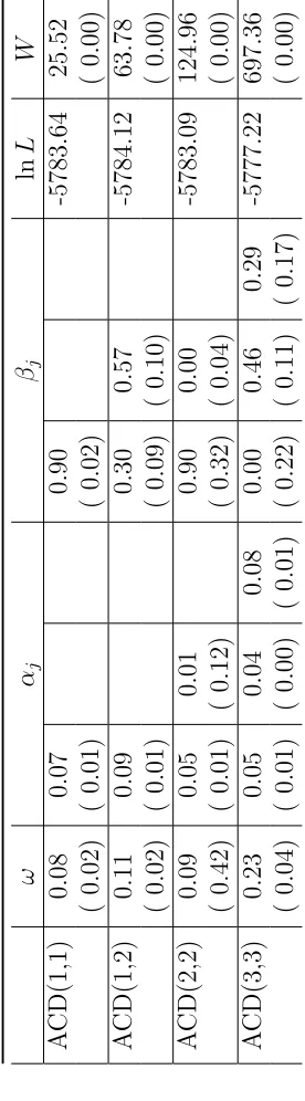
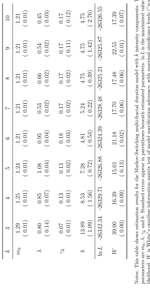
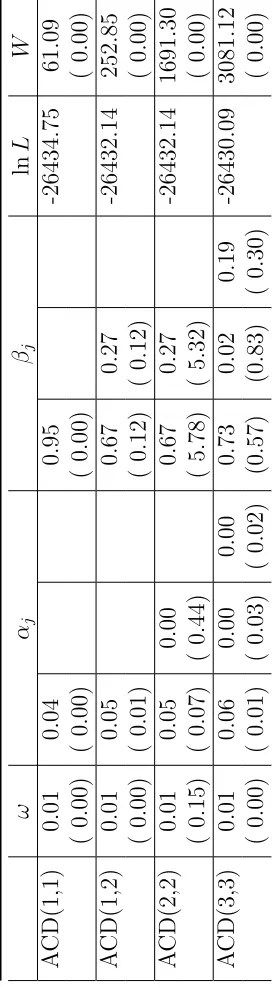
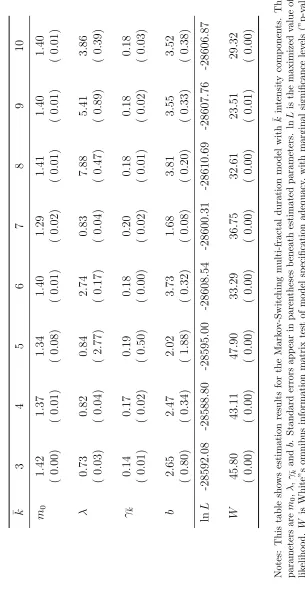
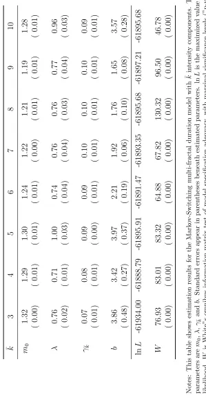
The binomial MSMD models with different ¯k are estimated for twenty stocks
randomly selected from the S&P 100 index. Table 1 gives the symbol and company
name of the twenty stocks. Empirical results show the MSMD mode with seven
intensity components, MSMD(7) can give a good description of the data. Four ACD
models, ACD(1,1), ACD(1,2), ACD(2,2) and ACD(3,3) are also estimated for the
same data. With number of parameters increasing from 3 to 7 when the model
changes from ACD(1,1) to ACD(3,3), the likelihood doesn’t decrease much. Thus
the ACD(1,1) is the leading model for ACD family.
model. Following Deo et al. (2010), I equally divide the twenty stocks into two
group-s, high trading group and low trading group, according to the number of transactions
in the sample period.I compare both in sample fitting and out of sample forecasting
of the two competing models. For in sample fitting, I compare the likelihoods.
Be-cause the two models are not nested and have different number of parameters, I use
Bayesian information criterion (BIC) to make a model selection. For out of sample
forecasting, I compare the mean square prediction errors for three horizons, 1-step,
5-step, and 20-step. A fixed scheme is chosen to compare forecasting performance,
see Pagan and Schwert (1990) and West and McCracken (1998) for more discussion
about this scheme. The detail is as follow: for stocks that have more than 11000
observations in the sampling period, I only take the first 11000 durations for
forecast-ing comparison. I split the 11000 durations into two sets, a fittforecast-ing set and a testforecast-ing
set. The fitting set has 10000 observations, and the later has 1000 observations. For
stocks that have less than 11000 observations, I take roughly the last 1000
observa-tion as testing set, all previous observaobserva-tions as fitting set. Competing models are
estimated only once on the fitting set and then the estimated parameters are used
in forming predictions for observations in the testing set. I choose this scheme
main-ly because the estimation processes of both models have computationalmain-ly intensive
numerical maximizations.
5.1
Data Description
The data for the empirical study are the consolidated trades data extracted from
TAQ database. The sample period is from February 1, 1993 to February 26, 1993,
which has 20 trading days. I only keep transactions during the open time, from 10:00
a.m. to 4:00 p.m.. All over night durations are omitted. Following Engle and Russell
(1998) and Zhang et al. (2001), transactions in the opening period from 9:30 am to
deleted as well.
5.2
Daily Seasonality
The raw durations have strong diurnal daily pattern, i.e., the average duration is
short both at opening time in the morning and at close time in the afternoon, but
long at noon time. This daily seasonality is documented by many empirical studies.
There are several methods to remove the seasonality. I adopt the method used by
Ghysels et al. (2004). The main step is to regress the logarithm of the raw duration
on the indicator variables that indicate the time of day. A day is divided into 12
subperiods. Each subperiod is 30 minutes. Consider the regression
logdi =
12
X
k=1
akxki+i =a0xi+i
where xki = 1, if timei belongs to the intraday subperiod k, and 0 otherwise. Then
the seasonally adjusted series is defined by
ˆ
di =diexp(−aˆ0xi)
where ˆa denotes the OLS estimator of a. The data from now on are all seasonally
adjusted data.
5.3
Data Statistics
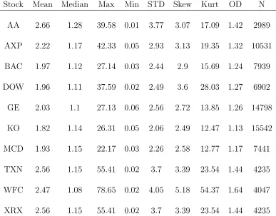
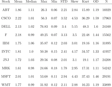
Table 2 and Table 3 show the summary statistics of durations for all twenty stocks.
The stock of Merck & Co is the most traded stock, which has 54242 durations in the
sampling period. While the stock of ALCOA is the least traded stock, having 2989
durations. The longest duration is 76.83. The shortest duration is 0.02. Durations
greater than median. Each stock’s duration kurtosis is much bigger than 3.
5.4
Estimation Method
The MSMD model is a hidden Markov model. The underlying Markov state variable
is the intensity state vectorMi. Every intensity component can take only two values
in the binomial MSMD model. The intensity state vector has ¯k components, thus
has 2¯k states. For finite number of states, likelihood of the model can be calculated
by standard filtering procedure.
The procedure is as follow: first initiate the distribution of Mi with its ergodic
distribution, then use Bayes’ law to update the distribution of Mi, and compute the
likelihood for each observation. MLE is used to estimate the four parameters. Like
other hidden Markov models, local maximums exist. Multiple initial conditions are
tried to find the MLE estimation.
5.5
Model Diagnostics
Several types of diagnostic tests have been developed in the literature to evaluate the
fast growing ACD models, see Li and Yu (2003), Fernandes and Grammig (2005),
Meitz and Ter¨asvirta (2006), Chen and Hsieh (2010). Unfortunately, the MSMD
model is a latent variable model. These tests can not be applied here. Instead, I
use the information matrix test developed by White (1982) as diagnostic test. The
test is based upon the asymptotic equivalence of the Hessian and outer product
forms of Fisher’s information matrix, when the model is correctly specified. All the
non-redundant elements of the information matrix (total 10 elements) are selected
5.6
Estimation Results
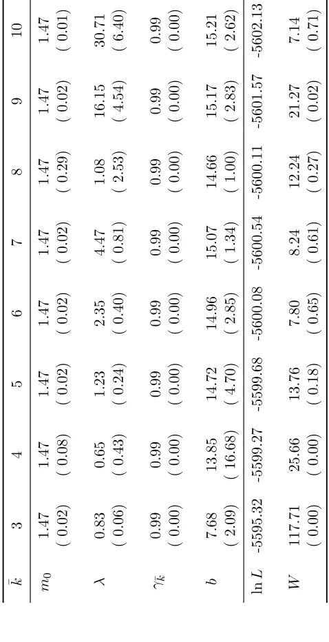
Both estimation results of MSMD and ACD models for all the twenty stocks are
presented in table 4 to table 43. For some low volume stock, γ¯k is very close to
1. Thus b and λ are weekly identified. This will cause some numerical instability.
In this case, I set γ¯k = 0.99 and maximize the likelihood through the other three
parameters.
The estimation results show: according to White’s omnibus information matrix
test, MSMD models are better fitted to the data than ACD models do, which is
obvious from the p value for both models. Within the ACD family, ACD(1,1) is the
best model. I thus choose to compare MSMD(7) and ACD(1,1) models.
5.6.1
Overdispersion Test
Engle and Russell (1998) develops an overdispersion test to diagnose the
exponen-tial ACD model and finds that the standardized durations still show overdispersion.
They conclude that the exponential errors are inadequate to capture the
overdisper-sion feature, then they try Weibull errors. But there is still overdisperoverdisper-sion. Many
researchers follow this excise and use more flexible error distributions. These
ex-ercises totally ignore the possibility that the misspecification of the GARCH-type
dynamics can also cause overdispersion. The empirical result here supports this
possibility.
The overdispersion test is as follow
√
N((ˆσ2−1)/√8)∼ N(0,1),
where N is the number of observations, ˆσ2
is variance of the standardized duration,
i.e., diˆλi. As I already mentioned when discussing model diagnostics, exact ˆλi is
not available in the MSMD model. But the distribution of the intensity state vector
the filtered distribution and the smoothed distribution. The expected λi can be
calculated from the two distributions, and they provide two approximations for λi.
The two approximations can be used to calculate the overdispersion test. Table 44
shows the the test statistics of both MSMD and ACD models for five stocks.
The test statistics of the ACD model for all five stocks are positive and the values
are out of the 90% confidence interval, which shows that there is still overdispersion
in the standardized durations. The test statistics of the MSMD model for all five
stocks are negative. The overdispersion feature is gone. This suggests that the
MSMD may explain the overdispersion in the data. But the statistics are still too
small and out of the 90% confidence interval. The reason could be that expected
λi, not the true value, is used to calculate the test statistics. The smoothed version
can usually give a better approximation to the true value than the filtered version,
and as one expects, the test statistics of the smoothed version are closer to the 90%
confidence interval than the filter version. Statistics of both versions for the MSMD
are closer to the confidence interval than the ACD.
From the above analysis, one can see that the overdispersion feature can be
cap-tured by the dynamic specification. There is no necessity to use flexible distributions.
5.6.2
Comparison with ACD
The MSMD model has been applied to real data and it can give a good description of
the data when the number of intensity components is seven. From now on, I fix the
number of components at seven and run a horse race between the MSMD(7) model
and the ACD(1,1) model. I choose the ACD(1,1) model because it is the leading
example of ACD models.
Table 45 and table 47 give the in sample fit and out of sample forecast results for
low trading group. Table 48 and table 50 give the in sample fit and out of sample
forecast results for high trading group.
ACD(1,1) for all twenty stocks. But comparison between non-nested models with
different number of parameters is tricky. Usually a criteria should include a penalty
term related to number of parameters. Standard methods are AIC and BIC. Here
I choose BIC which puts more penalty on the number of parameters. Table 46 and
table 49 show BIC comparison for all twenty stocks. One can see the MSMD model
fit the data better than the ACD model.
For 1-step forecasting, the performance of both MSMD and ACD model is
com-parable. MSMD does slightly better forecasting for the high trading group, while
ACD(1,1) can give a little more precise forecasting for the low trading group.
For 5-step and 20-step forecasting, the MSMD model dominates the ACD model
for all 20 stocks. The forecasting gain by using MSMD is huge.
This is clear evidence that the ACD model can only capture short run dynamics,
while the MSMD can capture longer horizon dynamics. An interesting observation
is that the mean square prediction error of the MSMD model doesn’t change much
when the forecasting horizon changes.
It may be more fare to compare the MSMD model with a long memory ACD
model. But as I discuss in last section, the fractional integrated ACD model doesn’t
have second order moment. It is not a long memory model in the usual sense.
Another possible candidate is the long memory stochastic duration (LMSD) model
of Deo et al. (2010). One problem with LMSD is that it does not allow iid exponential
errors1. This contradicts with the discussion in section 2. So I don’t consider the
LMSD model.
1As Deo et al. (2010) reports that when applying the LMSD model to some data, their algorism
Chapter 6
Concluding Remarks
The intertrade duration is a natural measure of market liquidity and its variability
is related to liquidity risk. In this dissertation, I propose a new model, the MSMD
model to analyze intertrade durations. Compared to the conditional mean modeling
of ACD models, my method focus on intensity modeling.
I first establish a mixture of exponentials representation for intertrade durations
from general PP theory, then model the intensity process as a MSM process. I show
the MSMD model has good properties. It can explain most of the stylized facts of
financial durations.
Extensive empirical study shows the MSMD model can do good long horizon
forecasting. my model could be used for the analysis of liquidity risk on financial
markets. For example, the MSMD model has decomposed shocks into different
frequency, and the high frequency shocks can be regarded as liquidity shocks. One
can use bayesian method to update the probability distribution of the high frequency
shocks thus get a measure of liquidity.
Another interesting direction for future work is to link durations, or intensities
to volatilities. The MSM volatility model of Calvet and Fisher (2004) has a lot of
similarities with the MSM duration model. An investigation of the link between
Table 1: Twenty Stocks: Symbol and Company Name
Symbol Company Name
AA ALCOA
ABT Abbott Laboratories AXP American Express Inc
BAC Bank of America Corp
CSCO Cisco Systems
DELL Dell
DOW Dow Chemical
F Ford Motor
GE General Electric Co.
IBM International Business Machines INTC Intel Corporation
JNJ Johnson & Johnson Inc
KO The Coca-Cola Company
MCD McDonald’s Corp
MRK Merck & Co. MSFT Microsoft
TXN Texas Instruments
WFC Wells Fargo
WMT Wal-Mart
Table 2: Basic Statistics: Low Trading Group
Stock Mean Median Max Min STD Skew Kurt OD N
AA 2.66 1.28 39.58 0.01 3.77 3.07 17.09 1.42 2989
AXP 2.22 1.17 42.33 0.05 2.93 3.13 19.35 1.32 10531
BAC 1.97 1.12 27.14 0.03 2.44 2.9 15.69 1.24 7939
DOW 1.96 1.11 37.59 0.02 2.49 3.6 28.03 1.27 6902
GE 2.03 1.1 27.13 0.06 2.56 2.72 13.85 1.26 14798
KO 1.82 1.14 26.31 0.05 2.06 2.49 12.47 1.13 15542
MCD 1.93 1.15 22.17 0.03 2.26 2.58 12.77 1.17 7441
TXN 2.56 1.15 55.41 0.02 3.7 3.39 23.54 1.44 4235
WFC 2.47 1.08 78.65 0.02 4.05 5.18 54.37 1.64 4047
XRX 2.56 1.15 55.41 0.02 3.7 3.39 23.54 1.44 4235
Table 3: Basic Statistics: High Trading Group
Stock Mean Median Max Min STD Skew Kurt OD N
ABT 1.86 1.11 26.3 0.06 2.21 2.84 15.89 1.19 16929
CSCO 2.22 1.01 56.3 0.07 3.52 4.53 36.29 1.59 17963
DELL 2.13 1.02 76.83 0.09 3.4 5.15 48.3 1.6 24160
F 2.18 0.99 49.25 0.07 3.13 3.5 22.48 1.44 15562
IBM 1.75 1.06 35.87 0.12 2.03 3.01 19.16 1.16 31895
INTC 1.81 1.0 50.38 0.15 2.41 4.17 34.57 1.33 41957
JNJ 1.72 1.03 29.56 0.08 2.01 3.1 19.1 1.17 24208
MRK 1.61 0.98 24.66 0.18 1.78 2.95 17.31 1.11 54242
MSFT 2.01 1.01 53.68 0.11 2.94 4.43 37.43 1.46 29191
WMT 1.77 0.99 31.92 0.12 2.11 2.88 16.23 1.19 33899
T able 4: Mo del Estimation: AA ¯k 3 4 5 6 7 8 9 10 m0 1.47 1.47 1.47 1.47 1.47 1.47 1.47 1.47 ( 0.02) ( 0.08) ( 0.02) ( 0. 02) ( 0.02) ( 0.29) ( 0.02) ( 0.01) λ 0.83 0.65 1.23 2.35 4.47 1.08 16.15 30.71 ( 0.06) ( 0.43) ( 0.24) ( 0. 40) ( 0.81) ( 2.53) ( 4.54) ( 6.40)
γ¯k
0.99 0.99 0.99 0.99 0.99 0.99 0.99 0.99 ( 0.00) ( 0.00) ( 0.00) ( 0. 00) ( 0.00) ( 0.00) ( 0.00) ( 0.00) b 7.68 13.85 14.72 14.96 15.07 14.66 15.17 15.21 ( 2.09) ( 16.68) ( 4.70) ( 2. 85) ( 1.34) ( 1.00) ( 2.83) ( 2.62) ln L -5595.32 -5599.27 -5599.68 -5600.08 -5600.54 -5600.11 -5601.57 -5602.13 W 117.71 25.66 13.76 7.80 8.24 12.24 21.27 7.14 ( 0.00) ( 0.00) ( 0.18) ( 0. 65) ( 0.61) ( 0.27) ( 0.02) ( 0.71) Notes: This table sho ws estimation results for the Mark o v-Switc hing m ulti-fractal duration mo del with
¯kin
T able 5: A CD Mo del Estimation: A A ω αj βj ln L W A CD(1,1) 0.08 0.07 0.90 -5783.64 25.52 ( 0.02) ( 0.01) ( 0.02) ( 0.00) A CD(1,2) 0.11 0.09 0.30 0.57 -5784.12 63.78 ( 0.02) ( 0.01) ( 0.09) ( 0.10) ( 0.00) A CD(2,2) 0.09 0.05 0.01 0.90 0.00 -5783.09 124.96 ( 0.42) ( 0.01) ( 0.12) ( 0.32) ( 0.04) ( 0.00) A CD(3,3) 0.23 0.05 0.04 0.08 0.00 0.46 0.29 -5777.22 697.36 ( 0.04) ( 0.01) ( 0.00) ( 0.01) ( 0.22) ( 0.11) ( 0.17) ( 0.00) Notes: This table sho ws estimation results for sev eral A CD mo dels: ψi = ω + P j αj di−
T able 6: Mo del Estimation: ABT ¯k 3 4 5 6 7 8 9 10 m 0 1.29 1.25 1.24 1.21 1.21 1.21 1.21 1.21 ( 0.01) ( 0.01) ( 0.01) ( 0.01) ( 0.01) ( 0.01) ( 0.01) ( 0.01) λ 0.80 0.85 1.08 0.95 0.53 0.66 0.54 0.45 ( 0.14) ( 0.07) ( 0.04) ( 0.04) ( 0.02) ( 0.02) ( 0.02) ( 0.03) γ ¯k 0.07 0.13 0.13 0.18 0.17 0.17 0.17 0.17 ( 0.01) ( 0.01) ( 0.02) ( 0.03) ( 0.02) ( 0.02) ( 0.11) ( 0.12) b 13.89 8.53 7.28 4.81 5.24 4.75 4.75 4.75 ( 1.09) ( 1.56) ( 0.72) ( 0.53) ( 0.22) ( 0.39) ( 1.42) ( 2.76) ln L -26342.34 -26329.71 -26326 .88 -26324.39 -26328.48 -26325.21 -26325.87 -26326.55 W 39.00 16.39 15.01 21.18 17.70 17.48 22.55 17.39 ( 0.00) ( 0.09) ( 0.13) ( 0.02) ( 0.06) ( 0.06) ( 0.01) ( 0.07) Notes: This table sho ws estimation results for the Mark o v-Switc hing m ulti-fractal duration mo del with
¯kin
tensit y comp onen ts. The mo del parameters are m 0 , λ ,
γ¯k
T able 7: A CD Mo del Estim ation: ABT ω αj βj ln L W A CD(1,1) 0.01 0.04 0.95 -26434.75 61.09 ( 0.00) ( 0.00) ( 0.00) ( 0.00) A CD(1,2) 0.01 0.05 0.67 0.27 -26432.14 252.85 ( 0.00) ( 0.01) ( 0.12) ( 0.12) ( 0.00) A CD(2,2) 0.01 0.05 0.00 0.67 0.27 -26432.14 1691.30 ( 0.15) ( 0.07) ( 0.44) ( 5.78) ( 5.32) ( 0.00) A CD(3,3) 0.01 0.06 0.00 0.00 0.73 0.02 0.19 -26430.09 3081.12 ( 0.00) ( 0.01) ( 0.03) ( 0.02) (0.57) (0.83) ( 0.30) ( 0.00) Notes: This table sho ws estimation results for sev eral A CD mo dels: ψi = ω + P j αj di−
T able 8: Mo del Estimation: AXP ¯k 3 4 5 6 7 8 9 10 m 0 1.38 1.34 1.30 1.31 1.27 1.27 1.27 1.27 ( 0.48) ( 0.02) ( 0.01) ( 0.01) ( 0.01) ( 0.01) ( 0.01) ( 0.01) λ 0.76 0.95 0.87 1.61 0.81 1.12 1.54 1.21 ( 1.12) ( 0.26) ( 0.07) ( 0.15) ( 0.04) ( 0.09) ( 0.41) ( 0.03) γ ¯k 0.79 0.94 0.99 0.95 0.99 0.99 0.99 0.99 ( 0.10) ( 0.28) ( 0.00) ( 0.01) ( 0.00) ( 0.00) ( 0.00) ( 0.00) b 30.70 29.10 12.69 20.68 10.24 10.26 10.26 10.26 ( 0.59) ( 4.69) ( 1.62) ( 0.18) ( 1.08) ( 0.57) ( 1.18) ( 1.11) ln L -17888.32 -17844.68 -17835 .35 -17843.72 -17829.99 -17829.99 -17830.28 -17830.28 W 29.73 28.11 7.64 19.56 10.16 7.18 8.14 7.22 ( 0.00) ( 0.00) ( 0.66) ( 0.03) ( 0.43) ( 0.71) ( 0.61) ( 0.70) Notes: This table sho ws estimation results for the Mark o v-Switc hing m ulti-fractal duration mo del with
¯kin
tensit y comp onen ts. The mo del parameters are m 0 , λ ,
γ¯k
T able 9: A CD Mo del Estim ation: AXP ω αj βj ln L W A CD(1,1) 0.00 0.03 0.97 -18042.24 45.77 ( 0.00) ( 0.00) ( 0.00) ( 0.00) A CD(1,2) 0.01 0.06 0.26 0.68 -18033.72 184.85 ( 0.00) ( 0.00) ( 0.03) ( 0.03) ( 0.00) A CD(2,2) 0.01 0.06 0.00 0.26 0.68 -18033.72 537.16 ( 0.00) ( 0.01) ( 0.01) ( 0.11) ( 0.10) ( 0.00) A CD(3,3) 0.01 0.06 0.01 0.00 0.00 0.69 0.23 -18033.78 1848.12 ( 0.00) ( 0.01) ( 0.01) ( 0.01) ( 0.25) ( 0.10) ( 0.21) ( 0.00) Note: This table sho ws estimation results for sev eral A CD mo dels: ψi = ω + P j αj di−
T able 10: Mo del Estimation: BA C ¯k 3 4 5 6 7 8 9 10 m 0 1.36 1.31 1.27 1.25 1.23 1.25 1.23 1.19 ( 0.01) ( 0.01) ( 0.01) ( 0.01) ( 0.01) ( 0.01) ( 0.01) ( 0.01) λ 1.16 1.09 1.02 0.93 0.89 0.60 0.61 0.79 ( 0.06) ( 0.05) ( 0.03) ( 0.05) ( 0.11) ( 0.04) ( 0.03) ( 0.04) γ ¯k 0.42 0.86 0.99 0.98 0.99 0.98 0.99 0.99 ( 0.06) ( 0.25) ( 0.00) ( 0.02) ( 0.00) ( 0.06) ( 0.00) ( 0.00) b 20.43 11.58 7.76 4.91 3.80 5.05 3.84 2.34 ( 0.24) ( 2.07) ( 0.43) ( 0.68) ( 0.33) ( 3.00) ( 0.25) ( 0.14) ln L -12917.76 -12910.83 -12910 .44 -12910.30 -12909.57 -12911.86 -12911.17 -12910.28 W 20.09 11.32 13.26 8.07 11.33 11.64 14.32 17.47 ( 0.03) ( 0.33) ( 0.21) ( 0.62) ( 0.33) ( 0.31) ( 0.16) ( 0.06) Notes: This table sho ws estimation results for the Mark o v-Switc hing m ulti-fractal duration mo del with
¯kin
tensit y comp onen ts. The mo del parameters are m 0 , λ ,
γ¯k
T able 11: A CD Mo del Estimation: BA C ω αj βj ln L W A CD(1,1) 0.04 0.06 0.92 -13073.60 66.04 ( 0.01) ( 0.00) ( 0.01) ( 0.00) A CD(1,2) 0.06 0.08 0.45 0.44 -13067.01 309.69 ( 0.01) ( 0.01) ( 0.09) ( 0.09) ( 0.00) A CD(2,2) 0.06 0.08 0.00 0.45 0.44 -13067.01 846.32 ( 0.47) ( 0.02) ( 0.11) ( 0.45) ( 0.41) ( 0.00) A CD(3,3) 0.06 0.09 0.00 0.00 0.55 0.04 0.30 -13063.56 1540.62 ( 0.01) ( 0.01) ( 0.02) ( 0.03) ( 0.22) ( 0.37) ( 0.23) ( 0.00) Notes: This table sho ws estimation results for sev eral A CD mo dels: ψi = ω + P j αj di−
T able 12: Mo del Estimation: CSCO ¯k 3 4 5 6 7 8 9 10 m 0 1.42 1.37 1.34 1.40 1.29 1.41 1.40 1.40 ( 0.00) ( 0.01) ( 0.08) ( 0.01) ( 0.02) ( 0.01) ( 0.01) ( 0.01) λ 0.73 0.82 0.84 2.74 0.83 7.88 5.41 3.86 ( 0.03) ( 0.04) ( 2.77) ( 0.17) ( 0.04) ( 0.47) ( 0.89) ( 0.39) γ ¯k 0.14 0.17 0.19 0.18 0.20 0.18 0.18 0.18 ( 0.01) ( 0.02) ( 0.50) ( 0.00) ( 0.02) ( 0.01) ( 0.02) ( 0.03) b 2.65 2.47 2.02 3.73 1.68 3.81 3.55 3.52 ( 0.80) ( 0.34) ( 1.88) ( 0.32) ( 0.08) ( 0.20) ( 0.33) ( 0.38) ln L -28592.08 -28588.80 -28595 .00 -28608.54 -28600.31 -28610.69 -28607.76 -28606.87 W 45.80 43.11 47.90 33.29 36.75 32.61 23.51 29.32 ( 0.00) ( 0.00) ( 0.00) ( 0.00) ( 0.00) ( 0.00) ( 0.01) ( 0.00) Notes: This table sho ws estimation results for the Mark o v-Switc hing m ulti-fractal duration mo del with
¯kin
tensit y comp onen ts. The mo del parameters are m 0 , λ ,
γ¯k
T able 13: A CD Mo del Es timation: C SCO ω αj βj ln L W A CD(1,1) 0.09 0.22 0.75 -29098.61 224.24 ( 0.00) ( 0.00) ( 0.00) ( 0.00) A CD(1,2) 0.09 0.22 0.75 0.00 -29098.93 495.91 ( 0.03) ( 0.06) ( 0.04) ( 0.03) ( 0.00) A CD(2,2) 0.14 0.22 0.12 0.23 0.38 -29097.89 2166.04 ( 0.03) ( 0.01) ( 0.06) ( 0.30) ( 0.23) ( 0.00) A CD(3,3) 0.10 0.21 0.05 0.00 0.64 0.00 0.07 -29095.49 2622.01 ( 0.02) ( 0.01) ( 0.04) ( 0.05) ( 0.24) ( 0.34) ( 0.16) ( 0.00) Notes: This table sho ws estimation results for sev eral A CD mo dels: ψi = ω + P j αj di−
T able 14: Mo del Estimation: DELL ¯k 3 4 5 6 7 8 9 10 m 0 1.40 1.36 1.37 1.32 1.32 1.32 1.33 1.37 ( 0.01) ( 0.01) ( 0.01) ( 0.01) ( 0.02) ( 0.00) ( 0.01) ( 0.04) λ 0.67 0.80 1.26 1.18 0.91 1.35 3.98 1.26 ( 0.02) ( 0.04) ( 0.09) ( 0.04) ( 0.07) ( 0.10) ( 0.28) ( 0.06) γ ¯k 0.08 0.09 0.10 0.11 0.10 0.11 0.11 0.10 ( 0.02) ( 0.01) ( 0.01) ( 0.01) ( 0.01) ( 0.00) ( 0.04) ( 0.01) b 4.18 3.45 3.80 2.75 2.59 2.76 3.02 3.91 ( 0.98) ( 0.66) ( 0.55) ( 0.15) ( 0.30) ( 0.07) ( 0.39) ( 0.19) ln L -37957.67 -37903.42 -37909 .02 -37899.56 -37898.92 -37900.40 -37904.81 -37910.09 W 63.21 35.57 35.94 11.09 7.37 5.76 11.45 32.59 ( 0.00) ( 0.00) ( 0.00) ( 0.35) ( 0.69) ( 0.83) ( 0.32) ( 0.00) Notes: This table sho ws estimation results for the Mark o v-Switc hing m ulti-fractal duration mo del with
¯kin
tensit y comp onen ts. The mo del parameters are m 0 , λ ,
γ¯k
T able 15: A CD Mo del Es timation: DELL ω αj βj ln L W A CD(1,1) 0.03 0.15 0.84 -38240.47 196.25 ( 0.00) ( 0.00) ( 0.00) ( 0.00) A CD(1,2) 0.04 0.17 0.71 0.11 -38237.83 760.43 ( 0.00) ( 0.01) ( 0.05) ( 0.04) ( 0.00) A CD(2,2) 0.04 0.17 0.00 0.71 0.11 -38237.83 2594.74 ( 0.01) ( 3.11) ( 0.28) ( 2.37) ( 1.35) ( 0.00) A CD(3,3) 0.04 0.17 0.00 0.00 0.74 0.02 0.05 -38236.88 3355.24 ( 0.01) ( 0.01) ( 0.15) ( 0.06) ( 0.85) ( 1.05) ( 0.11) ( 0.00) Notes: This table sho ws estimation results for sev eral A CD mo dels: ψi = ω + P j αj di−
T able 16: Mo del Estimation: DO W ¯k 3 4 5 6 7 8 9 10 m 0 1.29 1.28 1.25 1.25 1.22 1.20 1.18 1.20 ( 0.01) ( 0.01) ( 0.01) ( 0.01) ( 0.01) ( 0.02) ( 0.02) ( 0.07) λ 0.72 0.64 0.64 0.51 0.90 0.88 0.60 0.92 ( 0.03) ( 0.02) ( 0.02) ( 0.02) ( 0.07) ( 0.11) ( 0.08) ( 0.18) γ ¯k 0.59 0.87 0.99 0.99 0.99 0.99 0.99 0.99 ( 0.10) ( 0.05) ( 0.00) ( 0.00) ( 0.00) ( 0.00) ( 0.00) ( 0.00) b 16.52 15.47 9.26 9.38 6.89 4.59 3.50 4.60 ( 0.41) ( 0.44) ( 1.37) ( 1.18) ( 0.27) ( 0.86) ( 0.38) ( 0.81) ln L -11159.40 -11149.76 -11146 .89 -11147.64 -11145.02 -11145.18 -11145.33 -11145.39 W 13.80 10.04 3.01 4.40 5.92 2.96 19.43 4.32 ( 0.18) ( 0.44) ( 0.98) ( 0.93) ( 0.82) ( 0.98) ( 0.04) ( 0.93) Notes: This table sho ws estimation results for the Mark o v-Switc hing m ulti-fractal duration mo del with
¯kin
tensit y comp onen ts. The mo del parameters are m 0 , λ ,
γ¯k
T able 17: A CD Mo del E sti mation: DO W ω αj βj ln L W A CD(1,1) 0.01 0.04 0.95 -11238.01 27.24 ( 0.00) ( 0.00) ( 0.01) ( 0.00) A CD(1,2) 0.02 0.05 0.75 0.19 -11237.46 64.51 ( 0.00) ( 0.01) ( 0.13) ( 0.13) ( 0.00) A CD(2,2) 0.03 0.03 0.04 0.00 0.91 -11237.33 62.96 ( 0.01) ( 0.01) ( 0.01) ( 0.03) ( 0.04) ( 0.00) A CD(3,3) 0.04 0.04 0.04 0.03 0.00 0.00 0.87 -11237.06 253.02 (0.01) ( 0.01) (0.01) (0.01) ( 0.06) (0.06) ( 0.05) ( 0.00) Notes: This table sho ws estimation results for sev eral A CD mo dels: ψi = ω + P j αj di−
T able 18: Mo del Estimation: F ¯k 3 4 5 6 7 8 9 10 m 0 1.43 1.37 1.35 1.32 1.30 1.30 1.27 1.27 ( 0.01) ( 0.01) ( 0.04) ( 0.01) ( 0.01) ( 0.04) ( 0.01) ( 0.01) λ 1.00 1.00 0.94 0.91 1.12 0.86 1.42 1.96 ( 0.09) ( 0.32) ( 1.16) ( 0.06) ( 0.02) ( 0.20) ( 0.10) ( 0.23) γ ¯k 0.76 1.00 1.00 1.00 1.00 1.00 1.00 1.00 ( 0.03) ( 0.02) ( 0.00) ( 0.00) ( 0.00) ( 0.00) ( 0.00) ( 0.00) b 19.68 13.82 14.82 8.55 6.85 6.84 5.71 5.72 ( 2.07) ( 2.68) ( 2.69) ( 1.00) ( 0.33) ( 3.08) ( 0.27) ( 0.80) ln L -25684.19 -25673.06 -25650 .57 -25640.26 -25638.54 -25638.98 -25635.94 -25636.67 W 55.32 16.75 22.23 11.29 15.59 16.38 18.44 17.15 ( 0.00) ( 0.08) ( 0.01) ( 0.34) ( 0.11) ( 0.09) ( 0.05) ( 0.07) Notes: This table sho ws estimation results for the Mark o v-Switc hing m ulti-fractal duration mo del with
¯kin
tensit y comp onen ts. The mo del parameters are m 0 , λ ,
γ¯k
T able 19: A CD Mo del Estimation: F ω αj βj ln L W A CD(1,1) 0.01 0.04 0.95 -26227.00 39.22 ( 0.00) ( 0.00) ( 0.00) ( 0.00) A CD(1,2) 0.01 0.06 0.52 0.41 -26215.05 410.60 ( 0.00) ( 0.01) ( 0.04) ( 0.05) ( 0.00) A CD(2,2) 0.01 0.06 0.00 0.52 0.41 -26215.05 2344.84 ( 0.01) ( 0.02) ( 0.10) ( 0.15) ( 0.22) ( 0.00) A CD(3,3) 0.01 0.08 0.00 0.00 0.46 0.00 0.45 -26195.72 1465.99 ( 0.01) ( 0.02) ( 0.04) ( 0.02) ( 0.37) ( 0.18) ( 0.43) ( 0.00) Notes: This table sho ws estimation results for sev eral A CD mo dels: ψi = ω + P j αj di−
T able 20: Mo del Estimation: GE ¯k 3 4 5 6 7 8 9 10 m 0 1.36 1.30 1.27 1.30 1.27 1.25 1.27 1.27 ( 0.02) ( 0.01) ( 0.01) ( 0.01) ( 0.01) ( 0.01) ( 0.15) ( 0.01) λ 0.90 0.85 0.80 1.75 0.51 0.56 0.96 2.30 ( 0.09) ( 0.03) ( 0.50) ( 0.10) ( 0.03) ( 0.01) ( 0.17) ( 0.16) γ ¯k 0.99 0.99 0.99 0.99 0.99 0.99 0.99 0.99 ( 0.00) ( 0.00) ( 0.00) ( 0.00) ( 0.00) ( 0.00) ( 0.00) ( 0.00) b 30.54 8.94 5.61 9.66 6.56 5.01 6.57 6.60 ( 3.12) ( 0.54) ( 0.41) ( 0.65) ( 0.46) ( 0.69) ( 2.79) ( 0.72) ln L -24406.93 -24404.04 -24406 .14 -24409.90 -24410.93 -24411.21 -24410.80 -24411.90 W 56.46 41.13 26.16 22.58 9.20 39.44 12.12 9.61 ( 0.00) ( 0.00) ( 0.00) ( 0.01) ( 0.51) ( 0.00) ( 0.28) ( 0.48) Notes: This table estimation results for the Mark o v-Switc hing m ulti-fractal duration mo del with ¯k in tensit y comp onen ts. The mo del pa-rameters are m 0 , λ ,
γ¯k
T able 21: A CD Mo del Estimation: GE ω αj βj ln L W A CD(1,1) 0.02 0.04 0.96 -24766.13 83.96 ( 0.00) ( 0.00) ( 0.00) ( 0.00) A CD(1,2) 0.03 0.06 0.31 0.62 -24754.82 274.33 ( 0.01) ( 0.01) ( 0.04) ( 0.04) ( 0.00) A CD(2,2) 0.03 0.06 0.00 0.31 0.62 -24754.82 956.88 ( 0.04) ( 0.16) ( 0.21) ( 1.87) ( 1.82) ( 0.00) A CD(3,3) 0.03 0.07 0.00 0.00 0.46 0.00 0.46 -24749.80 1817.35 ( 0.01) ( 0.01) ( 0.02) ( 0.01) ( 0.25) ( 0.24) ( 0.25) ( 0.00) Notes: This table sho ws estimation results for sev eral A CD mo dels: ψi = ω + P j αj di−
T able 22: Mo del Estimation: IBM ¯k 3 4 5 6 7 8 9 10 m 0 1.27 1.24 1.21 1.21 1.18 1.18 1.18 1.18 ( 0.01) ( 0.01) ( 0.03) ( 0.12) ( 0.01) ( 0.01) ( 0.01) ( 0.01) λ 0.82 0.87 0.84 1.06 0.77 0.65 0.56 0.67 ( 0.02) ( 0.03) ( 0.29) ( 0.33) ( 0.03) ( 0.03) ( 0.02) ( 0.02) γ ¯k 0.05 0.05 0.05 0.05 0.06 0.07 0.07 0.07 ( 0.00) ( 0.00) ( 0.01) ( 0.04) ( 0.02) ( 0.01) ( 0.01) ( 0.01) b 10.12 5.93 3.90 4.00 2.85 2.91 2.94 2.92 ( 0.99) ( 0.56) ( 1.91) ( 3.64) ( 0.31) ( 0.32) ( 0.27) ( 0.05) ln L -47744.73 -47710.78 -47696 .20 -47697.22 -47695.07 -47695.88 -47696.65 -47696.11 W 40.16 16.37 5.86 9.93 3.42 4.02 3.46 4.09 ( 0.00) ( 0.09) ( 0.83) ( 0.45) ( 0.97) ( 0.95) ( 0.97) ( 0.94) Notes: This table sho ws estimation results for the Mark o v-Switc hing m ulti-fractal duration mo del with
¯kin
tensit y comp onen ts. The mo del parameters are m 0 , λ ,
γ¯k
T able 23: A CD Mo del Estimation: IBM ω αj βj ln L W A CD(1,1) 0.01 0.05 0.95 -47794.69 164.63 ( 0.00) ( 0.00) ( 0.00) ( 0.00) A CD(1,2) 0.01 0.06 0.56 0.37 -47788.35 721.45 ( 0.00) ( 0.00) ( 0.00) ( 0.00) ( 0.00) A CD(2,2) 0.01 0.06 0.00 0.56 0.37 -47788.35 3483.86 ( 0.01) ( 0.02) ( 0.01) ( 0.29) ( 0.25) ( 0.00) A CD(3,3) 0.01 0.07 0.00 0.00 0.56 0.25 0.12 -47787.06 4477.01 ( 0.01) ( 0.01) ( 0.02) ( 0.01) ( 0.25) ( 0.24) ( 0.25) ( 0.00) Notes: This table estimation results for sev eral A CD mo dels: ψi = ω + P j αj di−
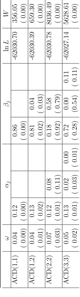
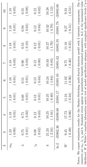
T able 24: Mo del Estimation: INTC ¯k 3 4 5 6 7 8 9 10 m 0 1.32 1.29 1.30 1.24 1.22 1.21 1.19 1.28 ( 0.00) ( 0.01) ( 0.01) ( 0.01) ( 0.00) ( 0.01) ( 0.01) ( 0.01) λ 0.76 0.71 1.00 0.74 0.76 0.76 0.77 0.96 ( 0.02) ( 0.01) ( 0.03) ( 0.04) ( 0.04) ( 0.03) ( 0.04) ( 0.03) γ ¯k 0.07 0.08 0.09 0.09 0.10 0.10 0.10 0.09 ( 0.01) ( 0.01) ( 0.00) ( 0.01) ( 0.01) ( 0.01) ( 0.01) ( 0.01) b 3.86 3.42 3.97 2.21 1.92 1.76 1.65 3.57 ( 0.48) ( 0.27) ( 0.37) ( 0.19) ( 0.06) ( 0.10) ( 0.08) ( 0.28) ln L -61934.00 -61888.79 -61895 .91 -61891.47 -61893.35 -61895.68 -61897.21 -61895.68 W 76.93 83.01 83.32 64.88 67.82 130.32 96.50 46.78 ( 0.00) ( 0.00) ( 0.00) ( 0.00) ( 0.00) ( 0.00) ( 0.00) ( 0.00) Notes: This table sho ws estimation results for the Mark o v-Switc hing m ulti-fractal duration mo del with
¯kin
tensit y comp onen ts. The mo del parameters are m 0 , λ ,
γ¯k
T able 25: A CD Mo del Estimation: INTC ω αj βj ln L W A CD(1,1) 0.04 0.12 0.86 -62030.70 356.05 ( 0.00) ( 0.00) ( 0.00) ( 0.00) A CD(1,2) 0.04 0.13 0.81 0.04 -62030.39 659.30 ( 0.01) ( 0.02) ( 0.02) ( 0.03) ( 0.00) A CD(2,2) 0.07 0.12 0.08 0.18 0.58 -62030.78 8036.49 ( 0.03) ( 0.01) ( 0.11) ( 0.92) ( 0.79) ( 0.00) A CD(3,3) 0.05 0.13 0.02 0.00 0.72 0.00 0.11 -62027.14 5628.61 ( 0.02) ( 0.01) ( 0.03) ( 0.01) ( 0.28) (0.54) ( 0.11) ( 0.00) Note: This table sho ws estimation results for sev eral A CD mo dels: ψi = ω + P j αj di−
T able 26: Mo del Estimation: JNJ ¯k 3 4 5 6 7 8 9 10 m 0 1.23 1.18 1.18 1.18 1.18 1.18 1.18 1.18 ( 0.00) ( 0.01) ( 0.01) ( 0.01) ( 0.03) ( 0.01) ( 0.01) ( 0.05) λ 0.75 0.71 0.60 0.51 0.90 0.53 0.94 0.55 ( 0.01) ( 0.02) ( 0.01) ( 0.01) ( 0.04) ( 0.10) ( 0.04) ( 0.08) γ ¯k 0.08 0.12 0.12 0.12 0.12 0.12 0.12 0.12 ( 0.02) ( 0.03) ( 0.01) ( 0.04) ( 0.00) ( 0.01) ( 0.04) ( 0.02) b 21.23 10.25 10.25 10.24 10.33 10.27 10.32 10.28 ( 2.34) ( 1.01) ( 0.40) ( 1.64) ( 0.83) ( 1.76) ( 4.70) ( 1.12) ln L -35902.36 -35890.60 -35891 .17 -35891.85 -35891.62 -35891.91 -35891.78 -35892.00 W 9.45 17.73 11.24 11.02 9.75 11.16 9.27 9.24 ( 0.49) ( 0.06) ( 0.34) ( 0.36) ( 0.46) ( 0.35) ( 0.51) ( 0.51) Notes: W e rep ort estimation results for the Mark o v-Switc hing m ulti-fractal duration mo del with ¯k in tensit y comp onen ts. The mo del pa-rameters are m 0 , λ ,
γ¯k
T able 27: A CD Mo del Esti mation: JNJ ω αj βj ln L W A CD(1,1) 0.00 0.02 0.97 -35961.84 89.46 ( 0.00) ( 0.00) ( 0.00) ( 0.00) A CD(1,2) 0.00 0.03 0.56 0.41 -35958.18 358.62 ( 0.00) ( 0.00) ( 0.03) ( 0.03) ( 0.00) A CD(2,2) 0.00 0.03 0.00 0.56 0.41 -35958.18 5051.19 ( 0.01) ( 0.02) ( 0.02) ( 0.85) ( 0.80) ( 0.00) A CD(3,3) 0.01 0.04 0.00 0.00 0.63 0.00 0.32 -35954.66 5628.00 ( 0.00) ( 0.00) ( 0.01) ( 0.02) ( 0.54) ( 1.00) ( 0.52) ( 0.00) Notes: This table sho ws estimation results for sev eral A CD mo dels: ψi = ω + P j αj di−
T able 28: Mo del Estimation: K O ¯k 3 4 5 6 7 8 9 10 m 0 1.24 1.21 1.20 1.21 1.18 1.21 1.18 1.21 ( 0.01) ( 0.52) ( 0.01) ( 0.34) ( 0.01) ( 0.38) ( 0.01) ( 0.01) λ 0.78 0.76 0.66 0.55 0.56 0.57 0.58 0.60 ( 0.02) ( 3.80) ( 0.02) ( 0.35) ( 0.09) ( 0.26) ( 0.02) ( 0.02) γ ¯k 0.33 0.65 0.72 0.75 0.85 0.75 0.86 0.75 ( 0.05) ( 0.49) ( 0.09) ( 0.57) ( 0.02) ( 0.26) ( 0.08) ( 0.41) b 12.02 7.21 6.78 7.17 4.69 7.23 4.78 7.23 ( 2.21) ( 2.89) ( 1.11) ( 8.03) ( 0.64) ( 3.19) ( 0.47) ( 1.23) ln L -24426.66 -24423.53 -24422 .53 -24423.63 -24424.36 -24423.97 -24424.81 -24424.15 W 25.44 23.20 12.45 12.75 13.51 11.88 13.47 11.27 ( 0.00) ( 0.01) ( 0.26) ( 0.24) ( 0.20) ( 0.29) ( 0.20) ( 0.34) Notes: This table sho ws estimation results for the Mark o v-Switc hing m ulti-fractal duration mo del with
¯kin
tensit y comp onen ts. The mo del parameters are m 0 , λ ,
γ¯k
T able 29: A CD Mo del Estimation: K O ω αj βj ln L W A CD(1,1) 0.04 0.04 0.93 -24534.83 148.40 ( 0.01) ( 0.00) ( 0.01) ( 0.00) A CD(1,2) 0.05 0.06 0.42 0.49 -24529.34 381.79 ( 0.02) ( 0.01) ( 0.07) ( 0.09) ( 0.00) A CD(2,2) 0.05 0.06 0.00 0.42 0.49 -24529.34 1480.63 ( 0.31) ( 0.31) ( 0.02) ( 0.82) ( 0.38) ( 0.00) A CD(3,3) 0.05 0.06 0.00 0.00 0.41 0.47 0.02 -24529.27 451.08 ( 0.01) ( 0.01) ( 0.01) ( 0.01) (0.03) ( 0.21) (0.07) ( 0.00) Notes: This table sho ws estimation results for sev eral A CD mo dels: ψi = ω + P j αj di−