https://doi.org/10.5194/nhess-18-2431-2018 © Author(s) 2018. This work is distributed under the Creative Commons Attribution 4.0 License.
A comparison of building value models for flood risk analysis
Veronika Röthlisberger1,2,3, Andreas P. Zischg1,2,3, and Margreth Keiler1,2
1Institute of Geography, University of Bern, Hallerstrasse 12, 3012 Bern, Switzerland
2Mobiliar Lab for Natural Risks, University of Bern, Hallerstrasse 12, 3012 Bern, Switzerland
3Oeschger Centre for Climate Change Research, University of Bern, Falkenplatz 16, 3012 Bern, Switzerland
Correspondence:Veronika Röthlisberger ([email protected]) Received: 13 December 2017 – Discussion started: 18 December 2017
Revised: 16 August 2018 – Accepted: 21 August 2018 – Published: 14 September 2018
Abstract.Quantitative flood risk analyses support decisions in flood management policies that aim for cost efficiency. Risk is commonly calculated by a combination of the three quantified factors: hazard, exposure and vulnerability. Our paper focuses on the quantification of exposure, in partic-ular on the relevance of building value estimation schemes within flood exposure analyses on regional to national scales. We compare five different models that estimate the values of flood-exposed buildings. Four of them refer to individ-ual buildings, whereas one is based on values per surface area, differentiated by land use category. That one follows an approach commonly used in flood risk analyses on re-gional or larger scales. Apart from the underlying concepts, the five models differ in complexity, data and computational expenses required for parameter estimations and in the data they require for model application.
The model parameters are estimated by using a database of more than half a million building insurance contracts in Switzerland, which are provided by 11 (out of 19) can-tonal insurance companies for buildings that operate under a monopoly within the respective Swiss cantons. Comparing the five model results with the directly applied spatially refer-enced insurance data suggests that models based on individ-ual buildings produce better results than the model based on surface area, but only if they include an individual building’s volume.
Applying the five models to all of Switzerland produces results that are very similar with regard to the spatial distri-bution of exposed-building values. Therefore, for spatial pri-oritizations, simpler models are preferable. In absolute val-ues, however, the five model results differ remarkably. The two simplest models underestimate the overall exposure, and even more so the extreme high values, upon which risk
man-agement strategies generally focus. In decision-making pro-cesses based on cost-efficiency, this underestimation would result in suboptimal resource allocation for protection mea-sures. Consequently, we propose that estimating exposed-building values should be based on individual exposed-buildings rather than on areas of land use types. In addition, a build-ing’s individual volume has to be taken into account in or-der to provide a reliable basis for cost–benefit analyses. The consideration of other building features further improves the value estimation. However, within the context of flood risk management, the optimal value estimation model depends on the specific questions to be answered. The concepts of the presented building value models are generic. Thus, these models are transferable, with minimal adjustments according to the application’s purpose and the data available. Within risk analyses, the paper’s focus is on exposure. However, the findings also have direct implications for flood risk analyses as most risk analyses take the value of exposed assets into account in a linear way.
1 Introduction
measures. Yet, measures entail costs, either in the form of direct construction expenditures or, indirectly, through lost profits due to restricted land use. However, budgets are gen-erally limited and thus they require measures be prioritized. This prioritization is based on quantitative flood risk analyses in many countries (Bründl et al., 2009; European Parliament, 2007).
In this context, risk is commonly defined as a combina-tion of hazard, exposure and vulnerability (see Birkmann, 2013 for an overview). It is usually expressed as the expected annual damage within a given area. There are different ap-proaches with which to estimate this expected annual dam-age. While models based on absolute damage functions com-bine exposure and vulnerability into one model component (e.g. Penning-Rowsell et al., 2005; Zhai et al., 2005), studies applying relative damage functions explicitly consider both the value and the physical vulnerability of exposed assets (e.g. Glas et al., 2017; Hatzikyriakou and Lin, 2017). The latter approach has the advantage of being more transparent than risk models with absolute damage functions. Our paper focuses on exposure, in particular on the relevance of build-ing value estimation schemes within flood exposure analyses on regional to national scales. However, as most risk analy-ses take the value of exposed assets into account in a linear way, this study’s results have direct implications for flood risk analyses, too.
Different studies (e.g. de Moel and Aerts, 2011; Koivumäki et al., 2010) show that uncertainties in quanti-tative flood risk analyses are driven rather by uncertainties in the value of exposed assets than by uncertainties in area or frequency of floods. This is especially true on regional to na-tional scales, where data availability limits the spatial resolu-tion and differentiaresolu-tion of asset values within flood exposure analyses. Aggregated classes of land use have been the norm (Gerl et al., 2016), at least until recently, and the area-specific value of each land use class is derived from lumped economic data of administrative units (Merz et al., 2010). This trans-formation of values per administrative unit into values per spatial unit differentiated by land use class implies spatial data disaggregation, also referred to as dasymetric mapping (Chen et al., 2004; Thieken et al., 2006). While several case studies investigate the influence that different data sources of asset values have on flood loss estimation (e.g. Bubeck et al., 2011; Budiyono et al., 2015; Cammerer et al., 2013; Jong-man et al., 2012), the effect of dasymetric mapping methods is only addressed in a few publications. For instance, Wün-sch et al. (2009) and Molinari and Scorzini (2017) show in local case studies that, even though the way in which exposed assets are estimated influences the resulting flood loss and thus flood risk, the spatial resolution of the exposed assets is more important. In both cases, the validation with recorded losses suggests that finer resolution of asset data improves the modelling results. Yet, both research teams conclude that further research on the impact of data resolution and disag-gregation is needed. In fact, based on the growing availability
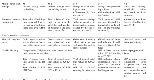
of high-resolution data and increasing computational power, more and more flood-risk-related studies on national scales are based on data at the building level (e.g. Fuchs et al., 2015, 2017; Jongman et al., 2014; Röthlisberger et al., 2017). How-ever, the individual monetary value of the buildings is usually not available due to data privacy restrictions and thus has to be estimated. There are different methods used in flood risk analyses to estimate individual building values (Jongman et al., 2014; Kleist et al., 2006). They range from uniform av-erage value per building to sophisticated regression models considering different building features. Yet, the role of these value estimation methods in flood risk assessments has re-ceived even less attention than the effect of dasymetric map-ping methods. To the best of our knowledge, no study has compared different object-based building value models, nor have these object-based methods ever been contrasted with the commonly used approaches of land-use-specific values per area within the context of regional or national risk anal-yses. To fill this gap, we investigate the influence of five dif-ferent value estimation models (called M1 to M5; see Ap-pendix A3 for an overview table of all abbreviations used in the text) on the resulting values of flood-exposed build-ings in Switzerland. Four of these models (M1, M2, M4 and M5; see upper most row in Table 1) refer to individual ings, whereas one model (M3) uses average values of build-ings per area, differentiated by land use category. The five models’ underlying concepts are widespread in risk manage-ment, construction industry and/or real estate management (see bottom row in Table 1). Apart from the concept, the five models mainly differ in their complexity and requirements on data resolution and differentiation.
Table 1.Overview of concepts, data and applications of the five investigated models for building value estimation. BFP stands for building footprint polygons, BZP for building zone polygons and PIC for points of insurance contracts.
Model name and concept
M 1
uniform average value per building
M 2
uniform average value per building volume
M 3
average value of build-ings per area, differentiated by land use category
M 4
average value per build-ing volume,
differentiated by build-ing features
M 5
value per building, individually calcu-lated based on linear regression
Parameter estima-tion and unit
Total value of buildings in an area divided by to-tal number of buildings in the same area, (CHF)
Total volume of build-ings in an area di-vided by total number of buildings in the same area, (CHF m−3)
Total value of buildings within an area of a par-ticular land use category divided by the size of the area, (CHF m−2)
Total value of build-ings with identical fea-tures divided by the vol-ume of the buildings, (CHF m−3)
Minimal adequate linear function of building fea-tures, (CHF)
Data for parameter estimation Minimal require-ment
Global sums of values and numbers of build-ings within a given area
Global sums of values and volumes of build-ings within a given area
Global sum of building values within an area with particular land use size of the area
Global sums of values and volumes of build-ings with identical fea-tures
Individual values and features of buildings
Used in this study Complete data of eight cantons where entire portfolio insurance data are available:
BFP of eleven cantons, reduced to polygons with joined PIC and matching volumes
(n=172 562) Total of insured
build-ings values in 529 224 PIC
Total number of BFP (391 766)
Total of insured build-ings values in 529 224 PIC
Total volume of BFP (653×106m3)
Total of insured build-ings values in 529 224 PIC
BZP of 12 408 km2, covering the entire area
BFP including volume, summarized value of joined PIC and infor-mation on land use and building purpose
BFP including volume, summarized value of joined PIC and information on land use, municipality type, building purpose and use
Data for bench-mark selection
The data must be spatially referenced at object level and complete within a given area.
In this study, we use the 529 224 PIC of the eight cantons, where complete portfolio data of the cantonal insurance company for buildings are available.
Data for model application Minimal require-ment
Individual buildings: lo-cation only
Individual buildings: lo-cation and volume
Land use:
spatially gapless infor-mation on land use cat-egories
Individual buildings: location, volume and features
Used in this study BFP data set of 2 086 411 footprints
BFP data set of 2 086 411 footprints, in-cluding volume
BZP of 41 290 km2, covering the whole of Switzerland
BFP data set of
2 086 411 footprints, including volume and information on land use and building purpose
Frequent fields of applications
Default values in tools for cost–benefit analyses of flood protection measures
Widely used in flood risk analyses on re-gional to national scales
Mainly used in construction industry and real estate management for the estimation of individual building construction costs
Examples DEFRA (2001); Wage-naar et al. (2016);
van Dyck and
Willems (2013)
BAFU (2015); de Bruijn et al. (2015); Mobiliar Lab (2016); Winter et al. (2018)
de Bubeck et al. (2011); Cammerer et al. (2013); ICPR (2001); Klijn et al. (2007); Thieken et al. (2008)
Hägi (1961); Naegeli and Wenger (1997);
SVKG and
SEK/SVIT (2002) Few applications in flood risk manage-ment, mainly at local level, e.g. Arrighi et al. (2013),
Lowe et al. (2006); Son-mez (2008)
To our knowledge no application in flood risk management
et al. (2016) shows that replacement costs are in fact the most often indicated cost base. Yet, there are risk analyses which use other types of building values, e.g. property prices (Ernst et al., 2010) or depreciated construction values (ICPR, 2001). However, this paper’s topic, which is the relevance of the model approach for the resulting value of exposed build-ings, does not depend on the value type and we thus refer to the literature (Merz et al., 2010; Penning-Rowsell, 2015) for broader discussions on building values in risk analyses.
2 Methods applied and data used
Sect. 2.4. Table 1 gives an overview of the five models with respect to their underlying concepts, data and applications.
2.1 Model set-up for value estimation
The five models in our study follow two different approaches. M3 is based on average value of buildings per area, differen-tiated by land use category. The other four models (M1, M2, M4 and M5) refer to individual buildings. These four mod-els are defined as follows: M1 is uniform average value per building; M2 is uniform average value per building volume; M4 is average value per building volume, differentiated by building features; and M5 is value per building, individually calculated based on linear regression. From M1 to M5, the complexity of the five models increases, as well as the data and computational expenses required for the estimation of their parameter values (see Table 1). The selection of the five models is driven by the data, which are available throughout Switzerland, as this paper is focused on analyses on regional to national scales. An additional selection criteria is the cur-rent application in risk management, construction industry or real estate management (see bottom line in Table 1). In the following, we outline the concepts of the five models and the estimation of their parameter values.
Model M1: uniform average value per building
Model M1 takes a straightforward approach as it assigns the same uniform average building value to each building. The parameter estimation requires two quantities with the same spatial aggregation, e.g. administrative units: (1) the total cu-mulative value and (2) the total number of buildings within the same area. By dividing the total building value by the to-tal number of buildings, we obtain the value of the model’s only parameter. The parameter corresponds to the average value of the buildings situated within the observed area. The unit of the M1 parameter is monetary value per building, e.g. (CHF).
Model M2: uniform average value per building volume Model M2 is based on the building volumes only. The data requirements for the parameter estimation are similar to the ones for M1. In place of the total number of buildings, M2 requires the total cumulative volume of buildings within a given area. To obtain the value of model’s only parameter, the total building value is divided by the total building volume. Thus, the parameter of M2 is defined as the average value per building volume and is given in monetary value per unit volume, e.g. (CHF m−3).
Model M3: average building values per area, differentiated by land use category
Model M3 takes a very common approach to flood risk anal-yses on national scales. It makes use of average building
val-ues per unit area, differentiated by land use category. For the same given area, the parameter estimation requires two comprehensive data sets of comparable spatial resolution: (1) gapless polygons of land use types and (2) spatially refer-enced data on building values. The two data sets are spatially joined, and the total building values per land use category are then calculated. In a last step, the cumulative building values per each type of land use are divided by the respective total area. This results in land-use-specific values of the model’s parameter. They correspond to the average monetary build-ing value per area of each land use category, which is given in monetary value per unit area, e.g. (CHF m−2).
Model M4: average values per building volume,
differentiated by land use category and building purpose Model M4’s parameter is the same as in M2, i.e. the average monetary value per building volume. In contrast, the param-eter values of M4 are not uniform but differentiated accord-ing to buildaccord-ing feature. In this study, land use category and building purpose are the criteria for differentiation. To esti-mate the specific parameter values of M4, we combine data on monetary value, volume, land use category and building purpose at the building level. These assignments at building level require inputting data of high spatial resolution and pre-cise localization. To estimate M4’s parameter values, the data assignments have to be complete for each individual build-ing. However, in contrast to M1, M2 and M3, the input data for M4 do not need to be comprehensive within a given area. For M4, only buildings with complete information on value, volume and the differentiation criteria are considered, and the value and volume of all buildings from the same combi-nation of differentiation criteria (e.g. same land use category and building purpose) are summed up. Finally, the cumulated monetary values are divided by the respective volumes, re-sulting in the model’s parameter values. Thus, we obtain one specific value for each combination of differentiation crite-ria. The parameter’s unit is monetary value per unit volume, e.g. (CHF m−3).
Model M5: value per building, individually calculated based on linear regression
of non-significant explanatory variables and interactions. In addition, we plot the model’s residuals to check visually if principal assumptions of linear regression on residuals are satisfied. The result of this exploratory process is the mini-mal adequate model that makes it possible to calculate the expected monetary value of a building as a linear function of the selected buildings attributes and interactions. This value is given in monetary units, e.g. (CHF).
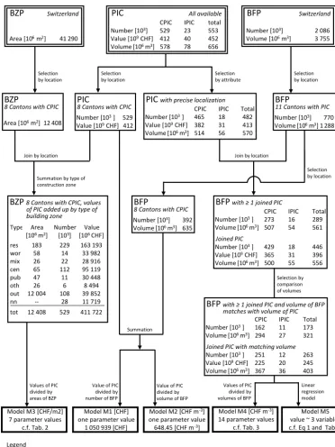
While the five applied models are conceptually different, the estimation of their parameter values in our study is based on the same data sets as much as possible. Nevertheless, the parameter estimation is based on two different kinds of data subsets. This is because the first three models (M1 to M3) re-quire a data selection, which fulfils different criteria in com-parison to the selection for M4 and M5. While the crucial prerequisite for M1, M2 and M3 is data completeness within a given area, the other two models require a high spatial accu-racy of the input data, mirrored in matching data assignments on individual building levels. Figure 1 shows the workflow of the set-ups of the five models for building value estimation.
2.2 Intersection with flood hazard maps and spatial aggregation
Based on the five described models, it is possible to calculate the monetary value of individual buildings (M1, M2, M4 and M5) or mean building values within predefined areas (M3). To identify the values which are exposed to floods, the build-ings or areas need to be spatially referenced and overlaid with flood hazard maps. The exposed values based on M3 are defined by the extent of flood-exposed areas and their respective monetary value per area. With regard to exposed values based on individual buildings, we classify a building as exposed to floods if it partially or entirely overlaps with a flood-prone area. From this exposed building, the entire mon-etary value is considered for the calculation of flood-exposed values. To compare the model based on areas (M3) with the other four models, we compile a map of regular hexagons with an area of 10 km2and calculate the sum of exposed val-ues per hexagon for all five models.
The described intersection with flood hazard zones re-duces the value of exposure to the buildings within flood-prone areas. In other contexts – in particular in the insurance industry, which provided data to this study (see Sect. 2.4.3) – exposure includes all assets or buildings, irrespective of the object’s individual chance of being damaged.
2.3 Selection of benchmark model and model comparison
Because our study mainly focuses on comparing different modelling approaches rather than on model predictions, we follow a benchmark test instead of a strict validation proce-dure. In a first step, we select a benchmark model that best fits the direct application of provided portfolio data of
can-tonal insurance companies for buildings within eight Swiss cantons. In a second step, we compare the other four models with the benchmark model and examine the distributions of the extreme high values in more detail, including their spa-tial distributions. In contrast to the selection of the bench-mark, the comparison of the benchmark model with the four other models covers the entire modelled area, i.e. the whole of Switzerland.
It is possible to select the model with the best fit in areas, where the data sets of the original building values are com-plete and spatially referenced on the building level. In our study, these areas correspond to the cantons, for which com-plete portfolio data of the cantonal insurance company for buildings are available; see Sect. 2.4.3. Within these cantons, we attribute the original building values from the portfolio data sets to the corresponding building geometries. Identify-ing flood-exposed buildIdentify-ings and summIdentify-ing the exposed values per hexagon are done in the same manner as for the building-based models. To identify the benchmark model, we examine differences and similarities between the model-based results and the results based on the original building values. For that matter, we calculate the root-mean-square errors (RMSE) and mean absolute errors (MAE) at the data aggregated to hexagons. We compile scatter plots of the hexagon values and compare the sum of exposed values over all hexagons within the validation area. As we are particularly interested in the distribution of the extreme high values, we further fit a generalized Pareto distribution (GPD) to the data above a certain consistent threshold. The threshold is the location pa-rameter of the GPDs. The other two GPD papa-rameters, the scale and shape, are estimated with the R package fExtremes (Wuertz, 2015) by applying the probability-weighted mo-ment method. Furthermore, we compare the highest hexagon values of each data set within the validation area.
2.4 Data
Each of the five generic models makes it possible to esti-mate flood-exposed-building values based on data sets that are available in many countries. However, the model set-up, especially the estimation of the parameter values, requires data sets on monetary building values, which are either rep-resentative of a given area (M1 to M3) and/or spatially ex-plicit (M3 to M5). In the following, Sect. 2.4.1, we present the input data of our study in Switzerland, and in Sect. 2.4.2 we detail the data selection for the parameter estimation. Sec-tion 2.4.3 shortly describes the data and area of model appli-cation and comparison.
2.4.1 Input data
Model M5 value ~ 3 variables c.f. Eq 1 and Tab. 4 Model M4 [CHF m-3]
14 parameter values c.f. Tab. 3 Model M3 [CHF/m2]
7 parameter values c.f. Tab. 2
Linear regression model
BZP Switzerland
Area [10 m ]6 2 41 290
PIC All available
CPIC IPIC total
Number [10 ]3 529 23 553
Value [10 CHF]9 412 40 452
Volume [10 m ] 5786 3 78 656
BFP Switzerland
Number [10 ] 3 2 086
Volume [10 m ] 3 7556 3
Selection by location
BZP
8 Cantons with CPIC
Area [10 m ] 12 4086 2
Selection by location
BFP
11 Cantons with PIC Number [10 ] 7703
Volume [10 m ] 1 2886 3 PIC
8 Cantons with CPIC Number [10 ] 5293
Value [10 CHF] 4129
Selection by location
Selection by attribute
PIC with precise localization CPIC IPIC Total Number [10 ] 4653 18 482
Value [10 CHF] 3829 31 413
Volume [10 m ] 5146 3 56 570
BFP with ≥ 1 joined PIC
CPIC IPIC Total Number [10 ] 2733 16 289
Volume [10 m ] 5076 3 54 561
Joined PIC
Number [10 ] 4293 18 446
Value [10 CHF] 3659 31 396
Volume [10 m ] 5006 3 55 556
Join by location
BFP
8 Cantons with CPIC Number [10 ] 3923
Volume [10 m ] 6356 3
Selection by location
Selection by comparison of volumes Join by location
Summation by type of construction zone
BZP 8 Cantons with CPIC, values of PIC added up by type of building zone
Type Area [106 m2]
Number [103]
Value [106 CHF]
res 183 229 163 193
wor 58 14 33 982
mix 26 22 28 916
cen 65 112 95 119
pub 47 11 30 448
oth 26 6 8 494
out 12 004 108 39 852
nn -- 28 11 719
tot 12 408 529 411 722
Values of PIC divided by areas of BZP
Value of PIC divided by number of BFP
Value of PIC divided by volume of BFP Summation
Values of PIC divided by volumes of BFP
Model M1 [CHF] one parameter value
1 050 939 [CHF]
Model M2 [CHF m-3]
one parameter value 648.45 [CHF m-3]
Legend
BZP: Building zone polygon PIC: Point of insurance contract BFP: Building footprint polygon res: residential, wor: working CPIC: Complete dataset of PIC
mix: mixed, cen: centre, pub: public IPIC: Incomplete dataset of PIC oth: other, out: outside building zone
nn: not known, tot: total
BFP with ≥ 1 joined PIC and volume of BFP matches with volume of PIC
CPIC IPIC Total
Number [10 ] 1623 11 173
Volume [10 m ] 2946 3 27 321
Joined PIC with matching volume Number [10 ] 2513 12 263
Value [10 CHF]9 225 20 245
Volume [10 m ] 3676 3 36 403
Figure 1.Workflow of the set-ups of the five investigated models for building value estimations.
used in the model application (see Table 1). The PIC data set is a compilation of 552 698 insurance contracts provided by eleven cantonal insurance companies for buildings (see Fig. 2), harmonized and expressed as values as per 2014. Of these eleven insurance companies, eight companies provided the whole portfolio data set from 2013, whereas the three
Figure 2.Overview of provided data by the cantonal insurance companies for buildings. Three insurance companies only provided data limited to contracts associated with at least one flood claim within the period indicated in brackets. The grey-shaded areas indicate the footprints of all buildings in Switzerland. Map source: Federal Office of Topography (swisstopo).
Table 2.Parameter values of the model M3, value per surface area (CHF m−2) of seven types of land use, i.e. six types of building zones and the area outside of building zones, based on a complete portfolio data of eight cantonal insurance companies for buildings in Switzerland. Insured values of buildings, which are localized at least on street level, are directly assigned to a type of land use. Values of the remaining buildings are split over all types of land use according to the size of the area of each type. The results per type of land use, which are used for further analyses, are in bold. Table entries are ordered by rank of these results.
Type of land use Area Value Value per area, directly assigned Value per area, total
(103m2) (103CHF) (CHF m−2) (CHF m−2)
Centre 64 974 95 118 671 1463.94 1464.88
Mixed 25 705 28 915 610 1124.89 1125.84
Residential 182 593 163 193 242 893.76 894.70
Public 47 323 30 448 192 643.42 644.36
Working 57 652 33 982 269 589.44 590.38
Others 25 593 8 493 504 331.87 332.81
Outside building zone 12 003 959 39 851 666 3.32 4.26
Not directly assigned – 11 719 182 – 0.94
Total 12 407 798 411 722 336 32.24 33.18
Cantonal insurance companies for buildings are present in 19 (of totally 26) Swiss cantons. In these 19 cantons, the in-surance of buildings is compulsory and provided by the re-spective cantonal insurance company for buildings, which operates under a legal monopoly. The claims are compen-sated at replacement costs; thus, the premiums are calculated based on replacement values. Consequently, the portfolio data of a cantonal insurance company for buildings include the replacement value of virtually every building within the respective canton. In addition, most contracts are located on the building level – in this study, this is true for 87 % of the
provided contracts – and often contain the volume of the in-sured building or building part. In our case, 78 % of the con-tracts include this information. The replacement values used and provided by the cantonal insurance companies for build-ings are object-specific estimates by experts. The values are based either (for new buildings) on documented construction costs such as invoices or (for older buildings) on on-site in-spection and validation.
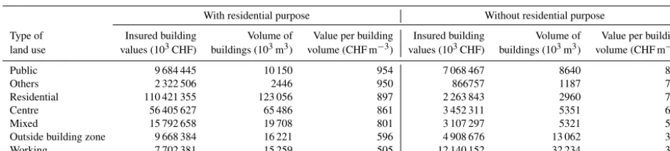
Table 3.Parameter values of model M4, value per volume (CHF m−3) above ground, differentiated according to the area’s land use where each building is located and by the purpose of the building. Calculations are based on insured values of 172 562 buildings, which are provided by eleven cantonal insurance companies in Switzerland. Table entries are ordered by the value per building volume of buildings with a residential purpose.
With residential purpose Without residential purpose
Type of Insured building Volume of Value per building Insured building Volume of Value per building land use values (103CHF) buildings (103m3) volume (CHF m−3) values (103CHF) buildings (103m3) volume (CHF m−3)
Public 9 684 445 10 150 954 7 068 467 8640 818
Others 2 322 506 2446 950 866757 1187 730
Residential 110 421 355 123 056 897 2 263 843 2960 765
Centre 56 405 627 65 486 861 3 452 311 5351 645
Mixed 15 792 658 19 708 801 3 107 297 5321 584
Outside building zone 9 668 384 16 221 596 4 908 676 13 062 376
Working 7 702 381 15 259 505 12 140 152 32 234 377
Table 4.Parameter estimates, standard errors, andtandpvalues of the three explanatory variables (and their pairwise interaction) of model M5. The three explanatory variables are residential purpose (ResPur) with values yes and no, the building volume above ground in m3 (volume) and land use (LaUse) with values residential, working, mixed, centre, public, others and outside (i.e. area outside building zones). The intercept stands for the variable values of log10(volume)=0 (i.e. volume=1 m3); ResPur=no and LaUse=outside.
Parameter Estimate Standard error tvalue P r(>|t|)
Intercept 3.097512 0.00633 489.334 <2.00E-16
ResPur yes 0.793809 0.007992 99.323 <2.00E-16
log10(volume) 0.80819 0.002385 338.9 <2.00E-16
LaUse residential −0.51207 0.009017 −56.79 <2.00E-16
LaUse working −0.4035 0.016537 −24.4 <2.00E-16
LaUse mixed −0.65351 0.015906 −41.087 <2.00E-16
LaUse centre −0.70887 0.009651 −73.453 <2.00E-16
LaUse public −0.44107 0.017177 −25.678 <2.00E-16
LaUse others −0.6658 0.027504 −24.208 <2.00E-16
ResPur yes×log10(volume) −0.15846 0.002694 −58.815 <2.00E-16 ResPur yes×LaUse residential −0.14691 0.003563 −41.23 <2.00E-16 ResPur yes×LaUse working −0.03614 0.005837 −6.192 5.95E-10 ResPur yes×LaUse mixed −0.05128 0.005654 −9.071 <2.00E-16 ResPur yes×LaUse centre −0.0001 0.003439 −0.029 0.977 ResPur yes×LaUse public −0.17378 0.006391 −27.19 <2.00E-16 ResPur yes×LaUse others −0.07611 0.011406 −6.673 2.52E-11 log10(volume)×LaUse residential 0.258569 0.003217 80.371 <2.00E-16 log10(volume)×LaUse working 0.158917 0.004704 33.787 <2.00E-16 log10(volume)×LaUse mixed 0.26366 0.004834 54.542 <2.00E-16 log10(volume)×LaUse centre 0.263382 0.003448 76.397 <2.00E-16 log10(volume)×LaUse public 0.256911 0.005323 48.262 <2.00E-16 log10(volume)×LaUse others 0.282637 0.009382 30.127 <2.00E-16
we reduce the nine provided building zone categories to six categories by merging the types “restricted building zones”, “zones for tourism and sports” and “transport infrastructure within building zones” to the type “other building zones”. Furthermore, we add the spatial complement of the building zones as “outside building zone” to the data set. Thus, we obtain a spatially gapless set of polygons with seven differ-ent types of building zones, namely “residdiffer-ential”, “working”, “mixed”, “centre”, “public”, “others” and “outside building zone”.
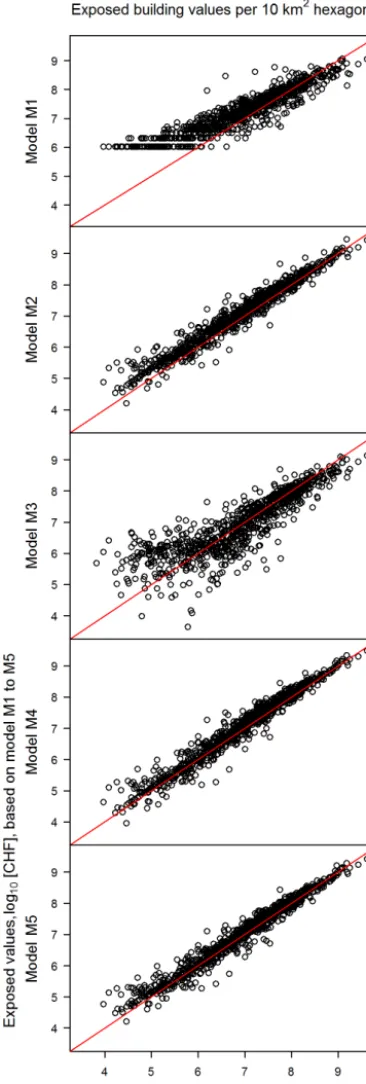
in-Figure 3.Scatter plot of flood-exposed-building values, aggregated to regular hexagons with a surface area of 10 km2. The sums based on models M1 to M5 (yaxis) are plotted against the sums based on the direct application of the values from the spatially referenced building insurance contracts (xaxis). The red lines indicate the 1:1 relation. The values are log10transformed and sums below 104CHF are not shown.
formation about residential purpose and use and (6) building densities in the BFP’s surroundings.
The calculation of flood-exposed-building values does not only require information on building values, but also on flood-prone areas. To define the areas potentially prone to in-undation in Switzerland, we combine two different types of flood maps. The main source is a compilation of all avail-able communal flood hazard maps in Switzerland (Borter, 1999; de Moel et al., 2009). These maps are collected, har-monized and provided in agreement with the responsible can-tonal authorities by the Swiss Mobiliar Insurance Company. We use the maps of December 2016, which cover 72 % of the buildings in Switzerland. In these maps, five different haz-ard levels are indicated, differentiated by the intensity (wa-ter depth and velocity) and probability of events (ARE et al., 2005). Out of the five hazard levels indicated in these maps, we consider the levels “major”, “moderate” and “low” as flood-prone areas. With the selection of these three lev-els, we include events up to a return period of 300 years. For the 28 % of the buildings in Switzerland that are not cov-ered by the communal flood hazard maps, we use the coarser flood map called Aquaprotect. This data set is provided by the Federal Office for the Environment (Federal Office for the Environment, 2008). Aquaprotect is available for the whole of Switzerland and contains four different layers with recur-rence periods of 50, 100, 250 and 500 years. For our study, we use the layer with the return period of 250 years. The compilation in GIS of the two map types follows the proce-dure described by Bernet et al. (2017) and results in a com-plete, nationwide map of flood-prone areas with return peri-ods of up to 250 (territories not covered by communal hazard maps) and 300 years (territories covered by communal haz-ard maps).
2.4.2 Data selection for the parameter estimation The workflow in Fig. 1 illustrates how the input data are com-bined and selected for the parameter estimation of the five models. The resulting data selection for each model is sum-marized in Table 1.
For M1 to M3, the two countrywide data sets (BFP for M1 and M2, BZP for M3) are reduced to the data entries, which are located within the eight cantons with complete building insurance data sets (left side of Fig. 1). In this way, the BZPs in the set-up of M3 cover 30 % of the data’s total coverage and the number of BFPs used for the parameter estimation of M1 and M2 correspond to 19 % of the total number of BFPs in Switzerland.
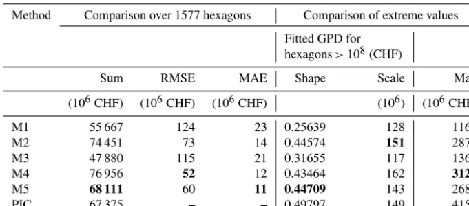
fur-Table 5.Indicators for the comparison of model M1 and M5 with the direct application of insurance data (insured values according to point-referenced building insurance contracts, PIC), in the eight cantons where complete portfolio data of the cantonal insurance companies for building are available. Sum represents the sum of exposed-building values over all 10 km2hexagons, RMSE and MAE represent the root-mean-square error and the mean-absolute error of exposed-building values per hexagon when comparing M1 to M5 with PIC. The generalized Pareto distribution (GPD) is fitted for hexagons with exposed-building values higher than 108CHF, which is equal to the location parameter of the GPD. Shape and scale represent the respective parameter of the fitted GPD. Max represents the highest sum of exposed-building values per hexagon. Bold numbers indicate the value (of M1–M5) nearest to the value based on PIC.
Method Comparison over 1577 hexagons Comparison of extreme values Fitted GPD for
hexagons>108(CHF)
Sum RMSE MAE Shape Scale Max
(106CHF) (106CHF) (106CHF) (106) (106CHF)
M1 55 667 124 23 0.25639 128 1163
M2 74 451 73 14 0.44574 151 2874
M3 47 880 115 21 0.31655 117 1367
M4 76 956 52 12 0.43464 162 3127
M5 68 111 60 11 0.44709 143 2682
PIC 67 375 – – 0.49797 149 4157
ther select the PICs that are localized at least at the street level, which is true for 95 % of the PICs in the eight can-tons with complete portfolio data. These PICs are spatially joined with the BZPs within the respective eight cantons. The monetary values of these PICs (CHF 400 billion total) are summarized per BZP type, and the values of the remain-ing PICs (i.e. CHF 12 million; see Fig. 1: BZP eight cantons with CPIC, values of PIC added up by type of building zone) are split proportionally to the area of each BZP category and added to the respective sum per BZP categories.
For M4 and M5, we reduce the original PIC data provided by eleven insurance companies to the 87 % of points with a localization on building level, and then we assign these points to the nearest BFP with GIS software (see Fig. 1: PIC all available → selection by attribute → PIC with precise lo-calization→join by location with BFP 11 cantons with PIC →BFP with≥1 joined PIC). 92 % of the PICs with a local-ization on building level can be matched to a BFP within a distance of less than or equal to 5 m. The attributes of these PICs, i.e. the replacement values and volumes of the insured buildings or building parts, are summarized per BFP. With this summation, the BFP with at least one joined PIC con-tains the attributes of the preprocessing steps (see description in Appendix A1), as well as the insurance-sourced building values and volumes. In particular, each of these BFPs in-cludes two types of building volume. The first type is the vol-ume above ground, calculated, in preprocessing steps, based on BFP area and the average height above ground of the building. The second type is the sum of volumes recorded in all PICs, which are assigned to the BFPs. For M4 and M5, we select only those BFPs for which the two mentioned vol-umes are within a predefined range (see Fig. 1: BFP with≥1 joined PIC→selection by comparison of volumes→BFP
with≥1 joined PIC and volume of BFP matches with vol-ume of PIC). For that matter, we calculate the volvol-ume ratio, i.e. the volume according to PIC divided by the BFP volume above ground. In the eight cantons, where we obtained com-plete portfolio data, we identify the volumes as matching if the volume ratio is equal to or more than 0.8 and less than or equal to 2.0. In the other three cantons, we set the lower crite-ria to equal to or more than 1.0. With this comparison of two independently derived volumes, we efficiently improve the quality of the BFP data. Particularly, we can exclude BFPs with inconsistencies in the calculation of the building vol-ume above ground and BFPs with mistakenly (not) assigned PICs, which thus have monetary values that are too high (or low). The exclusion of these BFPs is crucial for the set-up of the regression model (M5) and cannot be done manually given the size of the data set. The described comparison of volumes reduces the BFPs and the joined PICs simultane-ously and in a similar way. While 60 % of the BFPs to which a PIC is assigned are finally used for the set-up of M4 and M5, the respective ratio of PICs amounts to 59 %.
2.4.3 Data and area of model application and comparison
area of 41 290 km2, thus covering all of Switzerland (see Ta-ble 1). The benchmark model is selected in the eight cantons where complete building insurance data sets are available; for the benchmark test, we again consider the entire territory of Switzerland.
3 Results and discussion
In this section, we first show the parameter values of the five building value models, M1 to M5 (Sect. 3.1), and then present the results of the benchmark selection and test. The overall discussion of the models in the last subsection (Sect. 3.4) complements the specific comments in the first three subsections.
3.1 Parameter values M1 and M2
The parameter values of the two models with a single, uni-form parameter are CHF 1 050 939 per building (M1) and 648.45 CHF m−3per volume above ground (M2). These val-ues are rather high compared to international literature data (DEFRA, 2001; de Bruijn et al., 2015; Wagenaar et al., 2016), mainly because of comparatively high building stan-dards and construction costs in Switzerland. For instance, Diaz Muriel (2008) finds that the price level index for con-struction in Switzerland is 20 % higher than the average of the (at that time) 27 EU member states. In addition to and in contrast with these other studies, we count attached buildings like terraced houses as only one building, and the parameter of M2 refers to the building volume above ground but in-cludes the costs for underground building volumes too.
M3 and M4
Table 2 shows the parameter values of M3, i.e. the monetary values of buildings per surface area (CHF m−2) of seven land use categories. Most notable are the value differences be-tween the areas inside and outside building zones. The value for the areas outside the building zones is only a very low percentage of the building zones’ values, i.e. between 0.3 % (for centre) and 1.3 % (for others). Within the building zones, the values show less variation; i.e. they differ by a maximal factor of 4.5 corresponding to the difference between the cat-egories others and centre. Two aspects determine the parame-ter value of a specific land use class in M3: firstly, the density (built volume per unit area) of buildings in this land use class and, secondly, the monetary value per built unit volume. The second aspect is at the core of model M4, and the respec-tive parameter values by land use type and building purpose (with or without residential purpose) are presented in Table 3. The monetary value per volume is higher for buildings with a residential purpose than for non-residential buildings, rang-ing between 17 % for residential and public buildrang-ing zones to
58 % for areas outside building zones. For residential build-ings, the values for different land use types do not vary more than by a factor of 1.9 (working to public) and by a factor of up to 2.2 for buildings without a residential purpose. The ra-tio between the highest and the lowest M4 parameter value is 2.5. This is the ratio between the value per volume referring to residential buildings in public building zones and the value per volume, referring to non-residential buildings outside the building zone.
The remarkably smaller variation in parameter values in M4 compared to the variation in M3 and the differences be-tween M3 and M4 in the ranking of land use types by param-eter values all suggest that the differences in building densi-ties have a much higher impact on the variation of M3 pa-rameters than the differences in monetary value per volume. This is especially true for the areas outside building zones, where the M4 values per volume are comparable to the val-ues within building zones. In contrast, the M3 parameter for the area outside building zones is not higher than 1.3 % of the lowest value within building zones. That low percent-age reflects a similarly low ratio between building densi-ties outside and inside building zones. However, the effect of building densities also dominates within building zones. For the centre and mixed building zones, the M4 values per volume are at rank four and five, while the M3 parameter values for these zones are at rank one and two. That means the M3 values per area for the centre and mixed building zones are highly ranked, not because of high monetary val-ues per built volume, but because these building zones are densely built-up. In contrast, comparing M3 and M4 param-eter values for the public and other zones suggests that the construction costs for the buildings in these zones are com-parably high, but the built volume per area is rather low. In the international literature, the monetary values of buildings per surface area (M3, e.g. Bubeck et al., 2011; ICPR, 2001; Kljin et al., 2007) and the construction costs per building vol-ume (M4, e.g. Arrighi et al., 2013; Fuchs et al., 2015) are re-markably lower than the values in this study. As in the case of M1 and M2, these differences can be explained mainly by differences in building standards and construction costs in Switzerland (Diaz Muriel, 2008). For M3, the relatively dense settlements within building zones in Switzerland are another reason for the comparably high values in our study. Regression model M5
Based on our data, the minimal adequate linear regression model for the estimation of building values is
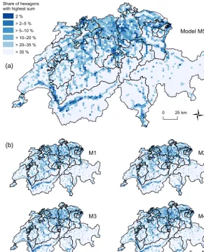
Table 6.Hexagons of 10 km2grouped in decreasing order of monetary values of flood-exposed buildings in Switzerland. For each group of hexagons and each model (M1 to M5) the following entities are reported: the lower limit of exposed-building values per hexagon (in 106 CHF), the sum (S* in 109CHF) of exposed-building values over all hexagons of the respective group, and the percentage (P∗in %) of this sum per group in relation to the total value of flood-exposed buildings in Switzerland. The spatial distribution of six of these groups (highest 2 %, lowest 65 % and four groups in between) are shown in Fig. 4.
Hexagon group Lower limit (106CHF) of Monetary value of exposed buildings per hexagon group: exposed-building values per hexagon sum [109CHF] and percentage (%) of total
Share (%) Number M1 M2 M3 M4 M5 M1 M2 M3 M4 M5
S* P∗ S* P∗ S* P∗ S* P∗ S* P∗
1 44 739 1518 827 1545 1409 48 14.1 112 21.9 57 18.4 127 23.6 107 22.8
2 89 590 1057 585 1114 980 77 23.0 168 32.8 88 28.4 185 34.4 158 33.6
5 222 353 550 344 565 500 137 40.8 268 52.4 146 47.0 287 53.5 248 52.8
10 444 224 303 197 306 274 200 59.4 358 70.1 204 65.7 380 70.7 330 70.2
20 889 108 129 88 134 119 270 80.3 447 87.3 264 85.2 471 87.8 412 87.5
35 1555 41 38 27 38 34 317 94.1 496 97.0 299 96.5 523 97.3 457 97.2
50 2222 12 7 5 6 6 333 99.0 509 99.6 308 99.5 536 99.7 469 99.7
100 4444 0 0 0 0 0 336 100 511 100 310 100 537 100 470 100
zones; see Sect. 2.4.1). The diagnostic plots of the model are presented in Appendix A2 and show that principal assump-tions regarding the residuals are satisfied. The coefficient of determination, adjustedR2, equals 0.88. In other words, M5 explains 88 % of the variance in the logarithmic monetary building values. The overall F statistic (60 000, on 21 and 172 degrees of freedom) results in apvalue<2.2×10⁻¹⁶, indicating an overall significance of the explanatory variables of M5. The estimates of the individual explanatory variables and their pairwise interactions are shown in Table 4, together with standard errors,tandpvalues. With one exception (Re-sPur yes×LaUse centre), all parameters of M5 are signifi-cant.
The intercept of 3.098 (=CHF 1250) refers to the vari-able values of log10(volume) =0, i.e. volume=1 m3,
Re-sPur = no and LaUse = outside. If the same theoretical building of 1 m3 has a residential purpose, the estimation of the monetary value increases by a factor between 4.2 (10(0.793−0.173)) in public building zones and 6.2 (100.793)
outside building zones or in centre zones. As building vol-ume increases, however, this factor between buildings with and without a residential purpose decreases and drops be-low 1 for building volumes between 8200 m3(public build-ing zones) and 102 000 m3(outside building zones). The ef-fects of land use categories other than outside and their in-teraction with building volumes are similar to the ones with residential purposes, but in the opposite direction. A theoret-ical building with a volume of 1 m3 in a building zone has a lower building value by factors 0.18 (10−(0.666+0.076) for other building zones, residential purpose) to 0.39 (10−0.404 for working zone, no residential purpose) compared to the same building outside building zones. With increasing ing volumes, these factors increase and exceed 1 for build-ing volumes between 52 m3(public building zones, no
res-idential purpose) and 584 m3 (working building zones, res-idential purpose). In any case, a higher volume of build-ings results in a higher building value, but for all buildbuild-ings with a residential purpose, the increase in value is lower than the increase in volume. Consequently, the ratio of dif-ference in value to difdif-ference in volume for residential build-ings within the same building zone is below 1. In fact, the ratio ranges from1volume−0.350for areas outside building zones to1volume−0.067for other building zones. For non-residential buildings, however, the increase in value is higher than the increase in volume in all building zones (with max-imal ratio of1volume0.091for other building zones), except for working building zone (1value=1volume−0.033) and for areas outside building zones where the difference in value equals1volume−0.192.
In summary, variable values that are different from the intercept generally increase the resulting monetary building values in M5:
– For ResPur, buildings with a residential purpose have a higher value than non-residential buildings, at least up to a volume of several thousand cubic metres.
– For LaUse, buildings in building zones are more expen-sive than comparable buildings outside building zones, but only if the buildings have a minimal volume of sev-eral dozen to a few hundred cubic metres, depending on land use and building purpose.
– Higher building volumes result in higher monetary building values, and for non-residential buildings in five building zones (residential, mixed, centre, public and others) the increase in value is higher than the increase in volume.
Share of hexagons with highest sum
Model M5
M1
1
M2
M3 M4
0 50 km 0 25 km
2 % > 2–5 % > 5–10 % > 10–20 % > 20–35 % > 35 %
(a)
(b)
Figure 4.Spatial distribution of flood-exposed-building values based on benchmark model M5 (uppermost figure) in addition to models M1 to M4 (lower figures). Hexagons with a surface area of 10 km2are categorized according to their sum of flood-exposed-building values. The specific limits of each category and the corresponding sums of exposed values are presented in Table 6. Map sources: Federal Office of Topography (swisstopo).
M4. M4 and M5 also agree in terms of LaUse, apart from working building zones. However, the findings on the differ-ent 1volume to1value relations in M5 do not support the concept of a constant value per volume ratio, which is used in M4.
In the following, we summarize the main reasons for excluding originally considered building features (building densities, residential use and municipality types) and for log-transforming the building volumes and values. The buildings densities are all highly correlated with building volume, but they explain less of the building values’ variance than the volume (lower adjusted R2, higher AIC). The same holds for residential use with respect to residential purpose. Mod-els that include municipality types and building zones con-tain many non-significant parameters. Models with munic-ipality types (but without building zones) explain less than corresponding models with building zones (but without
mu-nicipality types). The building volumes and values are log-transformed since the unlog-transformed values are right skewed and the residuals of models based on untransformed values are heteroscedastic.
3.2 Comparison of models with direct application of insurance data for benchmark model selection The eight cantons with complete insurance portfolio data cover an area of 12 408 km2. The corresponding layer of reg-ular 10 km2hexagons contains 1577 hexagons. Each point in Fig. 3 represents one of these hexagons. The log10values of
flood-exposed buildings summarized per hexagon based on value models M1 to M5 (y axis) are plotted against the ex-posed log10values based on the direct application of the
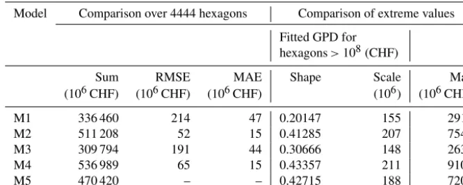
Table 7.Indicators for the comparison of model M1 to M4 with benchmark model M5. Sum represents the sum of exposed-building values over all hexagons, RMSE and MAE represent the root-mean-square error and the mean-absolute error of exposed-building values per hexagon when comparing M1 to M4 with M5. The generalized Pareto distribution (GPD) is fitted for hexagons with exposed-building values higher than 108(CHF), which is equal to the location parameter of the GPD. Shape and scale represent the respective parameter of the fitted GPD. Max represents the highest sum of exposed-building values per hexagon.
Model Comparison over 4444 hexagons Comparison of extreme values Fitted GPD for
hexagons>108(CHF)
Sum RMSE MAE Shape Scale Max
(106CHF) (106CHF) (106CHF) (106) (106CHF)
M1 336 460 214 47 0.20147 155 2912
M2 511 208 52 15 0.41285 207 7546
M3 309 794 191 44 0.30666 148 2634
M4 536 989 65 15 0.43357 211 9102
M5 470 420 – – 0.42715 188 7201
The exposure values per hexagon based on the M2, M4 and M5 models differ hardly by more than a factor of 101from the respective value based on direct PIC application. More-over, the factors are homoscedastic. The results from M1 and M3, however, differ by up to a factor of 102from the ones based on direct insurance data application. In addition, the factors for small values are clearly bigger than the factors for high values. Moreover, in M1 the values of hexagons with only a few exposed buildings are generally overestimated, and the hexagons with one or two exposed buildings appear as two horizontal lines (at 1.05×10⁶ and 2.1×10⁶CHF), with only seven hexagons in which the direct application of PIC results in higher exposure values than based on M1. In contrast, the values in hexagons with the most exposed build-ings are underestimated in M1. Hexagons with high exposure values are underestimated by the other four value models too, although this is less pronounced in the cases of M2, M4 and M5 than in M1 and M3.
The data in Table 5 support these findings quantitatively. Overall, the indicators for the models M1 and M3 show the least agreement with the values based on directly applied PICs. The sum of exposed values over all 1577 hexagons is closest to the PIC-based result in M5 (+1 %), and the sum differs most in M3 (−29 %). M4 shows the least RMSE and M5 the least MAE, and for both indicators, the values of M1 and M3 are approximately twice as high as the ones of the other three models. Comparing extremely high values again shows a clear division into two groups: M2, M4 and M5 ver-sus M1 and M3. The GPD fitted for hexagons with exposed-building values higher than 108 CHF show the best match with PIC-based extreme values for M2 and M5. The shape parameter determines the weight of the tail in the GPD, and it is highest in the case of direct PIC application, followed by the ones based on M5 (−10.2 %) and M2 (−10.4 %). This general underestimation of extremely high values by the five models is also reflected in the maximal exposure values,
where the models result in−25 % (M4) to−72 % (M1) lower values compared to the direct PIC application.
Based on these results, we select M5 as the benchmark model for comparing the countrywide model applications presented in the following section.
3.3 Benchmark test: differences and similarities between the five models
The summarized value of all flood-exposed buildings in Switzerland is between 3.1×10¹¹(M3) and 5.4×10¹¹CHF (M4). Based on the benchmark model M5, it is 4.7× 10¹¹CHF. The ratio between the highest and the lowest sums is thus 1.7, and the ratios to the benchmark model are be-tween 0.7 and 1.1. Table 6 presents the exposure values per eight ranked groups of the total 4444 regular hexagons cov-ering Switzerland. The table demonstrates that, for all five models, the distributions of exposed values per hexagon are clearly right skewed, but for M1 and M3 the skewness is less pronounced. This skew to the right implies that the expo-sure values of a few 10 km2hexagons represent an important part of the total value of flood-exposed buildings in Switzer-land. For instance, the 2 % (89) hexagons with the highest ex-posure values based on M5 contain flood-exposed buildings with a value of 1.6×10¹¹CHF, which corresponds to 33.6 % of the total value exposed in the whole of Switzerland based on M5. This share of exposed values in the 98th percentile is comparable for values from M2 (32.8 %) and M4 (34.4 %), but remarkably lower for M1 (23 %) and M3 (28.4 %). Com-paring the absolute values of the most exposed hexagons re-sults in the division of the same two clusters, down to the 95th percentile, the exposure values based on M2, M4 or M5 are approximately twice as high as the ones based on M1 or M3.
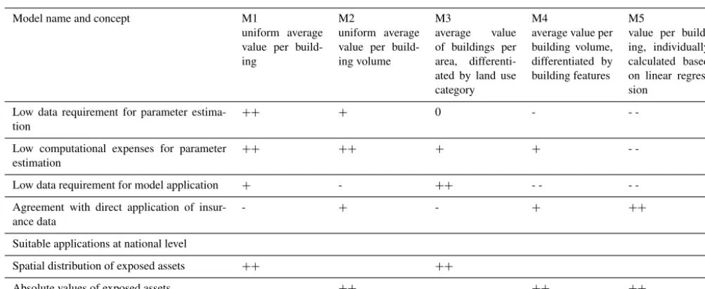
exposed-Table 8.Overview of core features and suitable applications of the five models. Symbols of characteristics:+is positive, 0 is neutral and minusis negative. The key figure in the online version of the article is a graphical version of this table.
Model name and concept M1
uniform average value per build-ing
M2
uniform average value per build-ing volume
M3
average value of buildings per area, differenti-ated by land use category
M4
average value per building volume, differentiated by building features
M5
value per build-ing, individually calculated based on linear regres-sion
Low data requirement for parameter estima-tion
++ + 0 -
-Low computational expenses for parameter estimation
++ ++ + +
-Low data requirement for model application + - ++ - -
-Agreement with direct application of insur-ance data
- + - + ++
Suitable applications at national level
Spatial distribution of exposed assets ++ ++
Absolute values of exposed assets ++ ++ ++
building values per hexagon are presented in columns three to seven in Table 6. The data again highlights the two groups: M2, M4 and M5 versus M1 and M3. However, the spatial dis-tribution of the 1555 (35 %) hexagons with the highest expo-sure values is very similar, with each of the five applied value estimation models. These hexagons cover wide areas in the northern part of Switzerland, but appear as isolated points or lines only in the southern part. Overall, the pattern mirrors the spatial settlement structure (see Fig. 2) in Switzerland, but the areas in the west as well as in the most eastern canton (i.e. GR) seem to exhibit a disproportionally low exposure, which confirms results by Fuchs et al. (2017).
The log–log plots presented in Fig. 5 show the flood-exposed values per hexagon based on the benchmark model M5 (x axis) against the values based on the other four mod-els (yaxis), with the red line indicating a one-to-one relation. In M2 and M4, the exposed values differ by not more than a factor of 5 from the respective values based on M5, whereas this factor goes up to 2×10²in M3 and to 5×101for M1. In addition, for M1 and M3, the factors are clearly bigger for lower exposure values than for higher ones, and high val-ues in both are generally underestimated. In contrast, the low exposure values in M1 are overestimated, and the values of hexagons with only a few exposed buildings appear as hori-zontal lines, similar to the pattern shown in the panel M1 of Fig. 3, as discussed above. The M2 panel suggests a general overestimation of the values compared to M5. Moreover, the differences are more pronounced for the middle ranges than for the extreme values. For the absolute deviations of M4 values from M5, no such dependency from the value’s rank can be detected, but the low values are underestimated, while high values are overestimated in M4.
Table 7 presents indicators when the M5 benchmark model is compared with the other four models. Overall, these indi-cators suggest that M2, closely followed by M4, best matches M5. In contrast, the exposure values based on M1 and M3 both agree much less with the M5 results. Compared to M5, M1 and M3 show a general underestimation of flood-exposed-building values, as well as an underestimation of the extreme high values. In contrast, M4 and, to a smaller de-gree, M2, overestimate the exposure values compared to M5. The parameters of the GPD fitted to hexagons with flood-exposed-building values higher than CHF 108are very simi-lar for M2, M4 and M5. Yet, the resulting empirical cumula-tive distribution functions presented in Fig. 6 for the highest two percent show that M2 matches better with M5 than M4.
3.4 Overall discussion of the five models
Based on the resulting values of flood-exposed buildings, the five models can be divided into two groups, one with M1 and M3 and another one with M2, M4 and M5 (see Table 8). Compared with the direct application of building values from PIC in eight cantons, M5 performs best. However, the results based on M2 and M4 are close, too, not only to the PIC re-sults in the eight cantons (see Sect. 3.2), but also to the M5 results over all of Switzerland (see Sect. 3.3). These three high-performing models include the building volume to es-timate the value, in contrast to M1 and M3. In other words, models which consider the building volume outperform the ones which do not include the volume, as long as there is a spread in the volume of the modelled building set.
Figure 5.Scatter plot of flood-exposed-building values aggregated to regular hexagons with a surface area of 10 km2. The sums based on models M1 to M4 (yaxis) are plotted against the sums based on the benchmark model M5 (xaxis). The red lines indicate the 1:1 relation. All values are log10transformed and sums below 104CHF are not shown.
Figure 6. Empirical cumulative distribution function of flood-exposed-building values aggregated to hexagons with a surface area of 10 km2. Cumulative probabilities (p) are generated by 105 ran-dom values from GPD with the parameters shown in Table 7. To improve the readability, only probabilities over 98 % are shown.
individual building level. However, the less detailed data re-quired in M1 to M4 differ too. While M1 and M2 require relatively simple data, i.e. global sums over a particular area such as administrative units, the sums of monetary building values required for M3 and M4 need to be differentiated to a higher degree. Consequently, the data requirements for the parameter estimation divide the models into three groups, with M1 and M2 in the group with the least requirements and M5 in the one with the most sophisticated requirements. The same grouping occurs when considering the computational expenses of the parameter estimations. While the parameter estimations in M1 and M2 each consist of one numerical di-vision, and in M3 and M4 of several divisions, the set-up of a linear regression model in M5 is an iterative and time-consuming process.
Grouping the models based on data requirements for the model application results in a distinction between M3 and the other four models (see Tables 1 and 8). Applying M3 re-quires spatially gapless data on land use, whereas the other four models need information on individual building levels for application. Among these four models, M1 requires the least information (location only), while M4 and M5 require the most information about each individual building, i.e. lo-cation, volume and other features. With regard to computa-tional expenses for the model application, the five models are similar.
of existing individual building value. On the other hand, M5 requires the most data and computational resources. With M1 and M3, it is the opposite. In summary, all five models have advantages and disadvantages, and when selecting a model there is a need to balance them. However, selecting a model is often driven by data availability in real-world applications. As this study shows, selecting a model has consequences for resulting exposure values.
4 Conclusions
The paper illustrates the role of building value models in flood exposure analyses on regional to national scales. The presented findings are relevant for flood risk analyses too, as most risk analyses take the value of exposed assets into account in a linear way. The study is based on insurance data; the used monetary building values represent replace-ment costs. However, the insights of this paper into the rel-evance of the model approach for the resulting value of ex-posed buildings are valid as well for other value types, as depreciated construction costs or property prices.
With regard to the spatial distribution of exposed-building values, the models show widely uniform results. In contrast, the absolute values of exposure differ remarkably. The first finding implies that the spatial prioritization of flood protec-tion measures would be similar with each of the applied value estimation methods. In practice, this means that the applica-tion of more sophisticated models does not generally pro-vide a better basis for spatial prioritizations. Consequently, simpler models with lower requirements regarding data in-put and comin-putational resources are preferable.
The second finding, however, suggests that decision-making processes that are based on cost–benefit criteria and thus rely on absolute monetary values are significantly influ-enced by which building value model one chooses. We find that models based on areas of land use classes, as commonly applied on regional to national scales, underestimate expo-sure values. The same is true for models based on individ-ual buildings that do not take the building volumes into ac-count. These two model types underestimate the overall ex-posure, but even more so the extremely high values on which risk management strategies generally focus. This underes-timation of the exposure value by models not considering the volume of buildings indicates that flood-exposed build-ings have in general a higher volume than buildbuild-ings outside flood zones. By underestimating exposed values, the bene-fits of protection measures (i.e. avoided flood losses) are un-derestimated as well. In decision-making processes that are based on cost efficiency, this underestimation would result in suboptimal allocation of resources for protection measures. Consequently, we propose that estimating exposed-building values should be based on individual buildings rather than on areas of land use types. In addition, and provided that there is a spread in the volume of the modelled building set, the
in-dividual volumes of buildings have to be taken into account in order to provide a reliable basis for cost–benefit analyses. The consideration of other building features further improves the value estimation.
In our study for the whole of Switzerland, with a data ag-gregation on 10 km2hexagons, the optimal model for the es-timation of absolute monetary building value is M5, i.e. a linear regression model considering the residential purpose and the building zone, in addition to building volume. In other contexts, where other data with different aggregations are available, the optimal building value model may be an-other one. For decisions that rely on absolute monetary build-ing values, however, our results suggest usbuild-ing a value model based on individual building data that in any case includes the building volume. The concepts of the three respective value models presented in this study, i.e. M2, M4 and M5, are generic. Thus, these models are transferrable with mini-mal adjustments according to the application’s purpose and the available data. However, within the context of flood risk management, the optimal value estimation model depends on the specific questions to be answered.
Growing availability of data with high resolution and spa-tial coverage in Switzerland and many other countries makes it possible to further develop complex multivariable build-ing value models, e.g. based on machine learnbuild-ing methods as done by Wagenaar et al. (2017) for the modelling of abso-lute flood damage. Depending on future data availability, it is also possible to extend the presented analyses to other assets of interest such as population or infrastructure. The compar-ison between different nationwide exposure analyses based on object-specific data including monetary values would be another promising approach for further research.
Appendix A
A1 Details on data and assignment of attributes to building polygons
Table A1 presents details on the data sets, which we use in our study aside from the insurance data described in Sect. 2.4. We assign the attributes to the building footprint polygons as follows.
A1.1 Building volume above ground
The building volume above ground is the product of the BFP area times the average building height above ground. While the calculation of a polygon’s area is a standard procedure in GIS, the estimation of the building height based on the available data is a multistep process. First, the points of the digital elevation model (swissALTI3D) and the digital sur-face model (DSM) are assigned to the polygons and for each polygon the two means of the assigned swissALTI3D points and DSM points are calculated. The subtraction of the mean of the DSM points from the mean from the swissALTI3D points results in the building’s average height above ground. If this height is ≥3.5 and≤100 m (which is the case for 1 378 665 of total 2 086 411 BFPs) it is used in the volume calculation, otherwise (n=707 746) it is adjusted as follows: for residential buildings (i.e. buildings with assigned residen-tial units as explained further down,n=232 016) the aver-age numbers of floors of the assigned BDS points (attribute GASTWS in BDS) is calculated, and for the first floor the height is set to 3.5 m and for each additional floor 2.5 m is added. For non-residential buildings with a height <3.5 m or>100 m (n=475 730) the value is set to 3.5 m.
A1.2 Type of building zone and type of municipality For the assignment of the types of building zones and mu-nicipalities, the positions of the building polygons’ centroids relative to the polygons in the data sets Bauzonen Schweiz and INFOFLAN-ARE are analysed. Prior to the assignment, in our study we reduce the types of building zones (attribute CH_BEZ_D in the data set Bauzonen Schweiz) from nine to seven types as described in Sect. 2.4.1. The types of mu-nicipalities (attribute TYP in INFOPLAN-ARE) are reduced from originally nine types down to six by merging the types “big centres” (code 1 in TYP), “secondary centres beside big centres” (2) and “middle centres” (4) to the type “big and middle centres” and by merging “belts of big centres” (3) and “belts of middle centres” (5) to the type “belts of big and middle centres”. Furthermore, we add the areas of lakes to the type “agricultural” (code 8 in TYP) municipality if they are not part of a municipality but of a canton. We obtain a spatially gapless set of polygons with six types of munici-pality, namely “big and middle centres”, “belts of big and middle centres”, “small centres”, “suburban rural
municipal-ities”, “agricultural municipalities and cantonal lake areas” and “tourist municipalities”.
A1.3 Binary information about residential purpose and use
The point data of residential units in the BDS (n=1 670 540) are joined to the next BFP (n=2 086 411) within 2 m. Ninety-seven percent (1 631 531) of the BDS points lay in or within a distance of 2 m to a BFP. We consider a BFP as a building with residential purpose if at least one BDS point is assigned to it (n=1 269 908 BFPs.) The criteria for res-idential use is that at least one person with main residence (attribute GAPHW in the BDS data set) is assigned to the building polygon, which is true for 1 129 904 BFPs.
A1.4 Building densities in the BFP surroundings For the calculation of the building density in the surrounding of a BFP we define circles of 50, 100, 200 and 500 m radius around the BFP’s centroid. For each of these circles we cal-culate the area of all BFP (cut to the circle’s edge) and divide it by the total area of the circle (cut to areas within Switzer-land and not covered by lakes). This way, for each BFP we obtain the building density in a circle 50 m (100, 200 and 500 m) around its centroid.
A2 Diagnostic plots of linear regression model M5 Figure A1 shows the diagnostic plots of M5, the minimal ad-equate linear regression model presented in Sect. 3.1. The two plots of residuals versus fitted values suggest (Fig. A1a and c) that residuals fulfil the assumptions of homoscedastic-ity, as the residuals are spread equally along the ranges of the fitted values. The quantile–quantile plot (Fig. A1b) indicates that the tales of the residuals’ distribution are heavier than in a normal distribution. Cook’s distance plot (Fig. A1d) shows that all buildings are inside Cook’s distance of 0.5, which means that no building significantly influences the resulting regression model. Overall it can be stated that the principal assumptions of linear regression modelling are reasonably satisfied.
A3 Abbreviations used in the text