www.atmos-meas-tech.net/7/1153/2014/ doi:10.5194/amt-7-1153-2014
© Author(s) 2014. CC Attribution 3.0 License.
Atmospheric
Measurement
Techniques
An improved algorithm for polar cloud-base detection by ceilometer
over the ice sheets
K. Van Tricht1, I. V. Gorodetskaya1, S. Lhermitte1,2, D. D. Turner3, J. H. Schween4, and N. P. M. Van Lipzig1
1KU Leuven, Department of Earth and Environmental Sciences, Leuven, Belgium 2Royal Netherlands Meteorological Institute (KNMI), De Bilt, the Netherlands 3NOAA National Severe Storms Laboratory, Norman, Oklahoma, USA
4Institute for Geophysics and Meteorology, University of Cologne, Cologne, Germany
Correspondence to: K. Van Tricht ([email protected])
Received: 8 October 2013 – Published in Atmos. Meas. Tech. Discuss.: 14 November 2013 Revised: 1 March 2014 – Accepted: 17 March 2014 – Published: 6 May 2014
Abstract. Optically thin ice and mixed-phase clouds play an
important role in polar regions due to their effect on cloud ra-diative impact and precipitation. Cloud-base heights can be detected by ceilometers, low-power backscatter lidars that run continuously and therefore have the potential to pro-vide basic cloud statistics including cloud frequency, base height and vertical structure. The standard cloud-base detec-tion algorithms of ceilometers are designed to detect opti-cally thick liquid-containing clouds, while the detection of thin ice clouds requires an alternative approach. This pa-per presents the polar threshold (PT) algorithm that was de-veloped to be sensitive to optically thin hydrometeor layers (minimum optical depthτ≥0.01). The PT algorithm detects the first hydrometeor layer in a vertical attenuated backscat-ter profile exceeding a predefined threshold in combination with noise reduction and averaging procedures. The optimal backscatter threshold of 3×10⁻⁴km−1sr−1for cloud-base detection near the surface was derived based on a sensitiv-ity analysis using data from Princess Elisabeth, Antarctica and Summit, Greenland. At higher altitudes where the aver-age noise level is higher than the backscatter threshold, the PT algorithm becomes signto-noise ratio driven. The al-gorithm defines cloudy conditions as any atmospheric profile containing a hydrometeor layer at least 90 m thick. A com-parison with relative humidity measurements from radioson-des at Summit illustrates the algorithm’s ability to signifi-cantly discriminate between clear-sky and cloudy conditions. Analysis of the cloud statistics derived from the PT algorithm indicates a year-round monthly mean cloud cover fraction of 72 % (±10 %) at Summit without a seasonal cycle. The
occurrence of optically thick layers, indicating the presence of supercooled liquid water droplets, shows a seasonal cy-cle at Summit with a monthly mean summer peak of 40 % (±4 %). The monthly mean cloud occurrence frequency in summer at Princess Elisabeth is 46 % (±5 %), which reduces to 12 % (±2.5 %) for supercooled liquid cloud layers. Our analyses furthermore illustrate the importance of optically thin hydrometeor layers located near the surface for both sites, with 87 % of all detections below 500 m for Summit and 80 % below 2 km for Princess Elisabeth. These results have implications for using satellite-based remotely sensed cloud observations, like CloudSat that may be insensitive for hydrometeors near the surface. The decrease of sensitivity with height, which is an inherent limitation of the ceilome-ter, does not have a significant impact on our results. This study highlights the potential of the PT algorithm to extract information in polar regions from various hydrometeor lay-ers using measurements by the robust and relatively low-cost ceilometer instrument.
1 Introduction
correctly projecting the polar climate, which is among others due to uncertainties in cloud parameterisations of macro- and microphysical properties (Bennartz et al., 2013; Ettema et al., 2010; Gorodetskaya et al., 2008) and feedback mechanisms (Dufresne and Bony, 2008).
Despite the great importance of clouds on the surface mass and energy balance, cloud research at high latitudes is still hampered by a lack of sufficient cloud observations. The harsh and remote environment of the Arctic and Antarctic has limited the amount of ground stations used for climatic re-search. The research sites that are present are equipped with robust instruments that can withstand very cold conditions. One of the most robust instruments that is used for observ-ing clouds is the ceilometer, a ground-based low-power li-dar device. It can operate continuously in all weather condi-tions (Hogan et al., 2003) and is one of the more abundant (>10) instruments at Arctic and Antarctic stations, includ-ing at Summit, Atqasuk, Barrow, Ny-Ålesund (Arctic study sites) and at Princess Elisabeth, Rothera, Halley (Antarctic study sites) (Bromwich et al., 2012; Shanklin et al., 2009; Shupe et al., 2011).
A macrophysical property inferred from ceilometer data is the cloud-base height (CBH) which is defined as the lower boundary of a cloud. The CBH is used for different pur-poses, including visibility determination, cloud height occur-rence statistics and validation of other remotely sensed cloud measurements, such as satellite observations. Most often, the CBH is calculated by built-in algorithms developed by the instrument’s manufacturers such as the Vaisala cloud-base detection algorithm (Garrett and Zhao, 2013; Shupe et al., 2011). These built-in algorithms are primarily designed to re-port the altitude where the horizontal visibility is drastically reduced from a pilot point of view (Flynn, 2004), which typ-ically occurs in liquid clouds. These algorithms are therefore not suited to detect base heights of optically thin ice clouds that frequently occur over the ice sheets. Bernhard (2004) showed that at the South Pole 71 % of all clouds have an op-tical depth below 1 and the Arctic clouds are also frequently optically thin (Sedlar et al., 2010; Shupe and Intrieri, 2004). Despite the low-optical depth of ice clouds, their detection is important in terms of determination of the cloud radia-tive impact or potential precipitation growth (Sun and Shine, 1995; Curry et al., 1996; Pruppacher and Klett, 2010; Kay and L’Ecuyer, 2013).
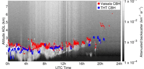
Ceilometers typically detect cloud bases in regions with high backscatter (see e.g. Fig. 1) that are likely related to liquid-containing portions in case of a mixed-phase cloud (Bromwich et al., 2012; Curry et al., 2000; Hobbs and Rangno, 1998; Pinto, 1998; Uttal et al., 2002; Verlinde et al., 2007). Yet, there are clearly regions with increased backscat-ter below. The optically much thicker top layer most proba-bly related to supercooled liquid has a much higher backscat-ter coefficient compared to the optically thin layer below. The conventional algorithms report this liquid cloud base, while detection of the ice cloud base below is also of great
Fig. 1. Ceilometer attenuated backscatter image at Princess
Elisa-beth (14 March 2011) on a logarithmic scale. Red dots represent the CBH calculated by the built-in Vaisala algorithm. Blue dots rep-resent the CBH calculated by the THT algorithm.
importance. There are also other CBH detection algorithms that use different approaches to infer CBH, for instance, the temporal height tracking (THT) algorithm developed by Martucci et al. (2010) that uses backscatter maxima and backscatter gradient maxima to calculate the CBH. Perfor-mance of the THT algorithm was shown to be superior for detecting warm liquid clouds, particularly when these clouds were rapidly changing in time. However, this algorithm has not been designed to detect optically thin clouds in a polar at-mosphere, which is apparent from the CBH detections by the THT algorithm in Fig. 1. Other more advanced instruments are also reporting CBH, such as the micropulse lidar (MPL) (e.g., Clothiaux et al., 1998; Campbell et al., 2002), but these instruments are less abundant over the different study sites in the Arctic and Antarctic, mostly due to their complexity, higher cost and the need for a manned station to operate such systems on site (Barnes et al., 2003). An algorithm that is ca-pable of calculating the CBH from ceilometer data in polar regions, including the detection of very optically thin ice lay-ers, therefore would greatly improve cloud statistics in these areas.
2 Data
2.1 Study area
The locations of the two research stations used in this study are shown in Fig. 2. They were chosen based on their char-acteristic climatology and available instrumentation.
The Antarctic data originate from the Princess Elisa-beth (PE) station (Pattyn et al., 2009), located in the es-carpment zone of Dronning Maud Land, East-Antarctica. The station is situated on the Utsteinen Ridge near the Sør Rondane mountains at an elevation of 1382 m a.s.l., 220 km inland (71.95◦S, 23.35◦E). Its location makes the
station well protected from katabatic winds; however, with a significant influence of coastal storms 50 % of the time (Gorodetskaya et al., 2013). Cloud measurements are car-ried out in the context of the HYDRANT project (the at-mospheric branch of the HYDRological cycle in ANTarc-tica), for which a unique instrument set has been installed, including a ceilometer, an uplooking infrared radiation py-rometer, a vertically pointing micro rain radar and an auto-matic weather station (Gorodetskaya et al., 2014). Data are currently limited to summertime cases due to power outages in wintertime. Cases used in this study are selected from De-cember to March between 2010 and 2013.
The Arctic cloud data were recorded at the Summit sta-tion atop the Greenland Ice Sheet, 3250 m a.s.l. (72.6◦N,
38.5◦W). The station is located 400 km inland from the
near-est coastline, making it a continental study site. The atmo-sphere on top of the ice sheet is extremely dry and cold, while many cloud properties are comparable to other Arc-tic regions (Shupe et al., 2013). The station is equipped with an extensive instrument set, including both passive as well as active sensors and a twice-daily radiosonde program, mak-ing this research site unique for cloud observmak-ing purposes. The cases used in this study are year-round measurements between 2010 and 2012 as part of the Integrated Character-ization of Energy, Clouds, Atmospheric state, and Precipita-tion at Summit (ICECAPS) project (Shupe et al., 2013).
2.2 Ceilometer
The Greenland Summit station is equipped with a Vaisala CT25K laser ceilometer, while the Antarctic PE station has the newer Vaisala CL31 laser ceilometer. Both instruments are emitting low-energy laser pulses and their vertical range extends up to 7.5 km. The CL31 instrument is more sensitive than the CT25K due to a higher average emitted power. Fur-ther technical details of both ceilometers are given in Table 1. The output used in this study is the range and sensitivity corrected attenuated backscatter coefficientβatt(km−1sr−1), which describes how much light from the emitted laser pulse is scattered into the backward direction, not corrected for attenuation by extinction. It is the product of the vol-ume backscatter coefficientβ at a certain height range and
" Princess Elisabeth
150°E
150°W 180°
60°S
60°S
"
Summit
20°W 40°W
60°W
70°N
60°N
0 500 1,000 Km 0 1,000 2,000
Km
¯
< 0 0 - 1,000
1,000 - 2,000 2,000 - 3,000
> 3,000 Altitude
(meters ASL)
Fig. 2. Locations of PE (Antarctica) and Summit (Greenland)
re-search stations.
the two-way attenuation of the atmosphere between the ceilometer and the scattering volume (Münkel et al., 2006). It is found after multiplying the received power by all in-strument specific factors (including a generic overlap correc-tion), constants and the squared distance. Since the transmit-tance of the atmosphere is in general unknown, conversion of the attenuated backscatter coefficientβattto the true volume backscatter coefficientβis not straightforward. The returned signal of the pulses is averaged over a period of 15 s which determines the temporal resolution of the measurements. The vertical resolution is 30 m for the CT25K at Summit and 10 m for the CL31 at PE.
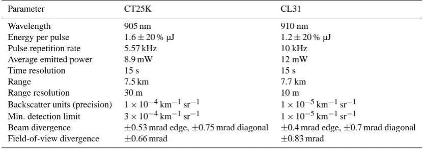
Table 1. Technical specifications of CT25K (Summit) and CL31 (PE) ceilometers.
Parameter CT25K CL31
Wavelength 905 nm 910 nm
Energy per pulse 1.6±20 % µJ 1.2±20 % µJ
Pulse repetition rate 5.57 kHz 10 kHz
Average emitted power 8.9 mW 12 mW
Time resolution 15 s 15 s
Range 7.5 km 7.7 km
Range resolution 30 m 10 m
Backscatter units (precision) 1×10⁻⁴km−1sr−1 1×10⁻⁵km−1sr−1 Min. detection limit 3×10⁻⁴km−1sr−1 1×10⁻⁵km−1sr−1
Beam divergence ±0.53 mrad edge,±0.75 mrad diagonal ±0.4 mrad edge,±0.7 mrad diagonal
Field-of-view divergence ±0.66 mrad ±0.83 mrad
value is 3×10⁻⁴km−1sr−1, while 1×10⁻⁵km−1sr−1is the minimum value reported by the PE ceilometer.
2.3 Radiosondes
Among the observations at Summit, twice a day a ra-diosonde program for characterising the atmospheric state is run (Shupe et al., 2013). Relative humidity (RH) is measured with the Vaisala RS92-K and RS92-SGP sondes and reported at a temporal resolution of 2 s, resulting in a vertical RH pro-file. Due to the low atmospheric temperatures, we report the RH with respect to ice (RHice), using Tetens formulation as described by Murray (1967). This formulation requires an extreme accuracy at low temperatures. The high uncertainty of the RH measurements at cold temperatures (dry bias) for the RS80 and RS90 sondes (Miloshevich et al., 2001; Rowe et al., 2008; Wang et al., 2013), is mostly resolved with the RS92 sondes (Suortti et al., 2008). Additionally, quantitative studies show that this issue is less severe in polar regions (Vömel et al., 2007), because the solar elevation angle is lower at high latitudes. Suortti et al. (2008) moreover iden-tified the RS92 sonde as being superior to other radiosonde sensors.
3 Polar threshold algorithm
The development of a CBH detection algorithm depends on atmospheric features considered to be a cloud. In this study a cloud is defined to be any hydrometeor layer at least 90 m thick in the atmospheric column detected by the ceilome-ter. Our new CBH detection algorithm determines the height of the first detectable occurrence of hydrometeors in a layer defined this way. We do not attempt to distinguish between clouds and precipitation, since our broad definition of a cloud and its importance for the energy and mass budget includes precipitation as well. This is different from the conventional algorithms that try to identify the base of the cloud above
the precipitation layer given that the latter does not entirely attenuate the signal.
Since our aim was to detect the CBH in optically thin lay-ers, even if liquid water droplets are present above them, the developed polar threshold (PT) algorithm compares the measured attenuated backscatter to a predefined backscat-ter threshold. This allows the algorithm to be sensitive to optically thin hydrometeor layers characterized by low at-tenuated backscatter returns and a lack of sharp gradients. This is an essential way by which our approach differs from both the standard Vaisala algorithm (Flynn, 2004) and the THT algorithm (Martucci et al., 2010) that look at visibil-ity or backscatter (gradient) maxima. In this section we first describe the noise reducing and averaging procedures to be carried out prior to the actual CBH detection, followed by the principles of the threshold approach and the procedure to determine the optimal backscatter threshold.
3.1 Noise reduction and averaging
For a sensitive algorithm to work properly, noise levels should be reduced and useful signal should be emphasized. The ceilometer being a low-power lidar inherently reports attenuated backscatter with a considerable degree of noise (e.g., Clothiaux et al., 1998). The fast decrease of signal with range and its range correction (evident from the lidar equa-tion in e.g. Münkel et al., 2006) leads to increasing noise lev-els higher in the profile. We therefore first remove noisy data detected by investigating the signal-to-noise ratio (SNR) and afterwards average the raw ceilometer attenuated backscatter data. The SNR was calculated for every separate height range bin at time stepiand range binj as
SNRi,j=
βi,j v
u u t 1
2M
+M
X
k=−M
βi+k,j−βi,j 2
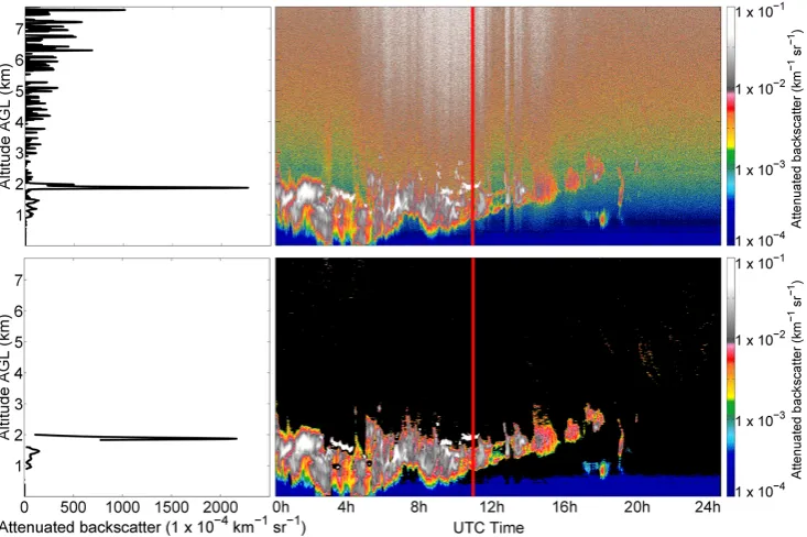
Fig. 3. Ceilometer attenuated backscatter (km−1sr−1) at PE (14 March 2011) with example profile, indicated by the red line, before (top) and after (bottom) noise reduction and averaging procedures. Negative noise values are not shown in the left figures. Range bins where the SNR<1 are not shown in the lower left image and are plotted in black in the lower right image.
which is the ratio of the temporal mean βi,j and standard deviation of the attenuated backscatter over±Mtime steps around time stepiand range binj.
Provided that the temporal resolution of the individual profiles is 15 s, M is equal to 20 profiles for a time inter-val of 10 min. The atmospheric fluctuations in this interinter-val are small compared to the instrument noise such that the standard deviation over the interval mainly contains internal noise from the instrument. This method is different from the common techniques used for lidars to estimate the ceilome-ter’s noise level from the background light (see e.g. Heese et al., 2010; Stachlewska et al., 2012; Wiegner and Geiß, 2012). In theory, the background light, reported as voltages by the Vaisala ceilometers, could be used to derive a rela-tionship with noise present in the data. In application to the polar atmosphere, however, this voltage is extremely small due to the low-solar zenith angle and low scattering in clear polar air. Therefore, we propose to work with the method as described in Eq. (1). Noisy data are characterized by a low mean backscatter (averaged over positive and negative ues) and a high standard deviation, resulting in low SNR val-ues. The SNR threshold was set to 1 as was also done by Heese et al. (2010), and pixels with a lower SNR were re-moved. The impact of this choice was assessed as well by varying this SNR threshold between 0.5 and 1.5. For the final analyses, the noise-reduced data were smoothed by applying a running mean over an interval of 2.5 min, determining the final temporal resolution of the data. Due to the impact of the averaging method on the results as reported in Stachlewska
et al. (2012), we varied the running mean interval between 1 and 15 min, but the impact on our results was below 1 %. Figure 3 shows an example ceilometer attenuated backscatter image with a typical backscatter profile before and after the noise reduction and averaging procedures.
3.2 Threshold approach
Attenuated backscatter
Altitude
A B C D E
SNR dr
iven
Thre
shold
driven
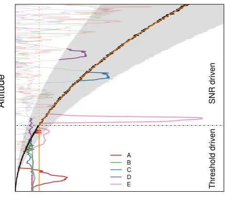
Fig. 4. Theoretical working of PT algorithm. The black curve
in-dicates the average noise level, increasing with height. The solid orange curve indicates the detection method in function of range as used by the PT algorithm. Five example backscatter profiles are in-dicated by curves A to E. The horizontal dashed black line shows the altitude above which the detection method becomes SNR driven. The shaded area represents variable detection sensitivity based on the SNR threshold.
in curves B to D in Fig. 4 that do not show cloud occurrence near the surface but would trigger a backscatter threshold that was set to the noise level.
To overcome this issue, we propose a CBH detection methodology based on an absolute attenuated backscatter threshold near the surface. This allows setting the threshold above the background value. Determination of the optimal threshold as indicated by the straight orange line in Fig. 4 is performed in Sect. 3.3. However, as range increases, the av-erage noise level increases accordingly. At a certain height (indicated by the horizontal dashed black line in Fig. 4), the noise level exceeds the backscatter threshold that was deter-mined near the surface where noise levels are small. Above this height, cloud detection by the ceilometer is limited by the noise present in the data. From this point onwards, cloud detection is therefore limited by the SNR, similar to the ap-proach by Platt et al. (1994), meaning that the PT algorithm then uses a threshold on the SNR for cloud-base detection. Due to the relatively low ceilometer power, noise levels in-crease with height and some optically thin ice clouds will be missed at high ranges, indicating that the sensitivity of the PT algorithm decreases with height above the point where the detection method becomes SNR driven.
The overall detection method used by the PT algorithm is thus split into two distinctly different parts depending on the height in the profile. This is indicated by the solid or-ange line in Fig. 4, indicating that the PT algorithm is driven
by a fixed attenuated backscatter threshold below the hori-zontal line where noise levels are very small, and driven by the SNR above the horizontal line, where noise levels be-come distinctly higher. If the noise reduction is based on a SNR threshold of 1 as determined in Sect. 3.1, this implies in practice that the backscatter of a cloud must be exceeding the noise level persistently in time to be identified as a cloud by the PT algorithm.
The SNR-threshold choice determines the tradeoff be-tween remaining noise in the data (lower SNR threshold) and loss of valid signal (higher SNR threshold) and therefore the sensitivity of the PT algorithm. We therefore evaluated the sensitivity on the results to SNR thresholds between 0.5 and 1.5. The PT algorithm then follows the margins of the shaded area around the noise level in Fig. 4. It is evident that using SNR threshold 0.5 allows the detection of optically thinner clouds (bold purple part in profile D), but introduces false triggering as well (profile B at the higher ranges). Setting the SNR threshold to 1.5 reduces false triggering in noise, but re-moves some thin clouds as well (bold blue part in profile C). Cloud statistics in Sect. 4.4 are therefore reported together with the sensitivity due the SNR-threshold choice.
Altitude AGL (km)
16h 17h 18h
1 2 3 4 5 6 7
Attenuated backscatter (km
−
1sr
−
1)
1 x 10⁻⁴ 1 x 10⁻³ 1 x 10⁻² 1 x 10⁻¹
−1000 0 1000 2000 3000
1 2 3 4 5 6 7
Altitude AGL (km)
Attenuated backscatter Vaisala CBH THT CBH PT CBH
UTC Time Attenuated backscatter (km−1sr−1)
Fig. 5. A time height cross section of the attenuated backscatter
coefficient (left) and a comparison between Vaisala (red), THT (blue) and PT (yellow) derived CBH in an example attenuated backscatter profile (indicated by red line in the left image) at PE on 14 March 2011 (right). Vaisala and THT report the CBH at high backscatter values. The PT algorithm is triggered at low backscatter values.
much lower backscatter values occurring at the base of an optically thin ice layer compared to the other algorithms that are triggered much higher in the profile, most probably at a liquid-containing layer. In the next section, the optimal backscatter threshold to be used by the PT algorithm is de-termined, in order to achieve results as in Fig. 5.
3.3 Determining optimal threshold
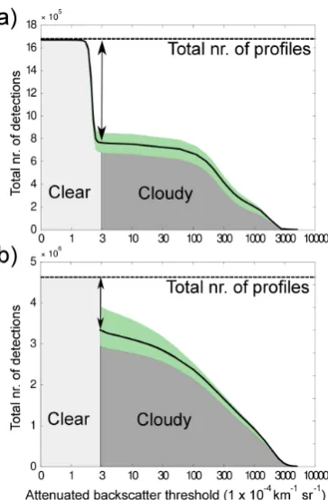
The CBH detection by the PT algorithm near the surface strongly depends on the backscatter threshold that is used. As discussed in Sect. 3.2, up to a certain altitude the backscat-ter threshold should not be based on the noise level to avoid false detections near the surface. The optimal threshold in this region is one that allows the detection of hydrometeor layers with a low optical depth while not triggering the algo-rithm in clear-sky conditions. To make an appropriate thresh-old choice, we performed a sensitivity analysis by varying the backscatter threshold between the detection limits of the ceilometers and the maximum backscatter value in the data and evaluating the effect on the cloud detections. The to-tal number of profiles containing a cloud that is detected by the PT algorithm over all cases (i.e. the total number of detections) was calculated for each threshold. The results of the sensitivity analysis for PE are shown in Fig. 6a. At a backscatter threshold just below 3×10⁻⁴km−1sr−1there is a sharp decrease in total number of detections. At this transition, the total number of detections is approximately halved, which is related to the fact that PE experiences syn-optic influence favouring cloud occurrence about 50 % of the time (Gorodetskaya et al., 2013). The backscatter threshold at 3×10⁻⁴km−1sr−1 effectively represents the minimum concentration of hydrometeors detectable by the ceilometer distinguishing cloudy from clear-sky profiles. The choice of the threshold at the sharp decrease in number of detections
Fig. 6. Sensitivity analyses of backscatter threshold on the cloud
detections for (a) PE and (b) Summit. The dashed line indicates the total amount of profiles that have been tested. The arrows show the amount of profiles marked as clear sky using the chosen threshold. The light grey area represents pixels reported as clear by the PT algorithm, while the dark grey area represents pixels reported as cloudy. The green areas represent uncertainty due to SNR-threshold choice.
is possible due to the clear polar troposphere and the neg-ligible ceilometer signal in the absence of clouds. A differ-ent relationship is expected for midlatitudes, for example, where the ceilometer signal near the surface will be sensi-tive to the presence of aerosols. The lowest detection limit after calibration of the ceilometer at Summit corresponds to the backscatter threshold determined for the PE ceilometer (Fig. 6b). Therefore, we used identical backscatter thresh-olds for PE and Summit. The shaded areas around the black curves indicate that the threshold choice is not very sensitive to the SNR threshold that was used.
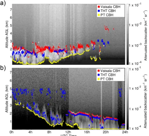
Fig. 7. Comparison of CBH detection results from Vaisala (red),
THT (blue) and PT (yellow) algorithms for (a) PE ceilometer case of 14 March 2011 and (b) Summit ceilometer case of 19 Decem-ber 2010.
threshold from 3×10⁻⁴km−1sr−1to 30×10−4km−1sr−1 at Summit decreases the amount of detections by 10 % and increases the mean CBH by 70 m, while at PE the amount of detections is decreased by only 2 %, though the mean CBH increases by 190 m. As our purpose is to detect the optically thinnest detectable hydrometeors lowest in the profile, we choose the lowest backscatter threshold indicating the pres-ence of hydrometeors (3×10⁻⁴km−1sr−1for both the PE and Summit ceilometers).
4 Results
4.1 Applying the PT algorithm
The PT algorithm was applied to all available cases at the study sites. Example CBH results for the three tested algo-rithms are shown in Fig. 7 with the 14 March 2011 case for PE (Antarctic autumn) and the 19 December 2010 case for Summit (Arctic winter). These cases were chosen because they represent different atmospheric conditions on which the PT algorithm could be tested. These conditions include clear-sky profiles, ice layers and polar mixed-phase cloud struc-tures (optically thicker layer most probably due to the pres-ence of supercooled liquid over an optically thinner but ge-ometrically thicker ice-only layer). The Summit ceilometer data in Fig. 7b indicate that precipitation reaches the surface after 14 h. Since the first 2 range bins of the profile were ex-cluded, the CBH is located at 60 m in such conditions.
In both cases, the mean PT CBH is significantly lower compared to the Vaisala and THT CBH. At both study sites,
the Vaisala CBH is mostly situated much higher in the cloud, where backscatter values are peaking. This is to be expected since the primary goal of the Vaisala algorithm is to detect visibility changes for pilots. In the case of optically thin fea-tures with only low backscatter values, Vaisala sometimes re-ports the profile as being clear sky (e.g. Fig. 7b from 00:00– 12:00 UTC). THT takes into account the first derivative of the backscatter profile, while optically thin ice clouds are not characterized by a sharp increase in backscatter. The THT CBH therefore is often placed higher as well. The PT algo-rithm is more sensitive and is triggered by optically thinner hydrometeor layers. The number of cloudy profiles reported by PT therefore is higher and the detected CBH is reported at lower altitudes. The sensitive nature of the PT algorithm indicates that the noise reduction and averaging procedures have to be an inherent part of the algorithm itself to avoid false triggering by noise in the signals.
4.2 Comparison with radiosondes
Fig. 8. Comparison between measured attenuated backscatter by
ceilometer (left) and RHice by radiosonde (right) at Summit on
5 August 2011.
at the same altitudes with an equal number of observations in each.
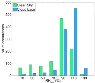
The histograms of the two samples (clear sky and cloud base) are plotted in Fig. 9. The green bars indicate occur-rences in a RHiceinterval for the clear-sky sample. Blue bars represent occurrences in a RHice interval for the cloud-base sample. It shows that when a cloud base is detected, the highest occurrences of RHice values at this cloud base are around 110 % with only very few cases lower than 90 %. For clear sky, on the other hand, the radiosonde also detects high RHice, although more occurrences at very low RHicevalues are present. The high abundance of large RHice values in clear-sky conditions is related to the high fraction of cloud bases near the surface (Sect. 4.4). Shupe et al. (2013) found that in this region RHicevalues are typically high due to the frequent occurrence of moisture inversions near the surface. According to Vömel et al. (2007), a possible dry bias in the RH measurements of the RS92 radiosonde is smallest at low altitudes, suggesting that our conclusions should not be in-fluenced significantly by a possible bias.
We used a one-sided nonparametric two-sample Kolmogorov–Smirnov test to determine if the RHice measurements of cloud bases were significantly higher compared to clear-sky RHice values (Hájek et al., 1967). The test indicates that the cloud-base RHice values are indeed significantly higher than the clear-sky RHice values (p value<0.01). If the PT algorithm would often be trig-gered in clear sky, both distributions would not statistically differ significantly which suggests that the PT algorithm performs well.
4.3 Optical depth of detected features
Translating the attenuated backscatter values of the de-tected hydrometeor layers to optical depths allows a phys-ical interpretation of what the PT algorithm actually de-tects. Such translation, however, is not straightforward since the optical depth depends strongly on the properties of
Fig. 9. RHice measurements of radiosondes for clear-sky sample
(green bars) and cloud-base sample (blue bars). For clear sky the same height distribution was followed as for cloud base. See text for more information.
the cloud (Tselioudis et al., 1992; King et al., 1998; Kay et al., 2006) and the calculation of optical depth requires the true backscatter coefficients and correction of the observed backscatter for attenuation of the signal is based on knowl-edge of the extinction profile which is unknown. The true backscatter coefficient was estimated following the proce-dure described by Platt (1979). This proceproce-dure starts with Eq. (2) that describes the relation between observed attenu-ated backscatter at a heightz(βatt,z) and the true backscatter
coefficient at this height corrected for attenuation (βz):
βz= βatt,z
exp(−2×τz)
. (2)
In this equation, the exponential term describes the two-way attenuation in the profile between the cloud base (z0) and heightzandτzis the optical depth along the path calculated
as
τz=
z Z
z0 σdz=
z Z
z0
S×βzdz, (3)
βz= βatt,z
exp−2×S×
z R
z0 βzdz
.
(4)
The procedure assumes that at the cloud baseβz0=βatt,z0,
since attenuation of the signal under the cloud base is negli-gible. Next, the cloud is divided into a number of layers, cor-responding to the range bins of the ceilometer. The integral in Eq. (4) is discretized and the true backscatter coefficients of the range bins are successively calculated until the upper end of the profile is reached. In the procedure, the effects of multiple scattering are not taken into account. In a final step, the optical depthτ of the detected cloud is cumulatively cal-culated for the successive range bins, using Eq. (3).
The assumptions for both the lidar ratio S and the derivation of the true backscatter coefficients from observed backscatter make the optical depth calculations prone to a considerable degree of uncertainty. Despite many assump-tions simplifying a complex problem, this procedure allows us to make a rough estimation of the optical depth of hydrom-eteor layers detected by the PT algorithm. We assessed the degree of uncertainty due to the lidar ratio approximation, by varying this ratioS between 16 sr< S <25 sr. The result-ing optical depth uncertainty was 25 %, which agrees well to similar studies with ceilometer (e.g., Wiegner and Geiß, 2012).
We found at Summit optical depths detected by the PT al-gorithm as low asτ =0.01 and 32 % of the detected hydrom-eteor features attenuated the laser beam (τ >3, in accor-dance with Sassen and Cho, 1992). At PE, the lower limit of optical depths was 0.01 as well, while 21 % of the detections attenuated the laser beam. The drawback of the high sensi-tivity of the algorithm (detection of features withτ =0.01) is that CBH detection can sometimes be triggered by layers of elevated aerosol contents. This only rarely happens over the Antarctic ice sheet due to its remote location and clean air (e.g., Hov et al., 2007). This is not the case for Green-land, which is much closer to industrialized countries. In the events of elevated aerosol contents, some aerosol layers will inherently be identified falsely as cloud (Shupe et al., 2011), an issue that occurs in other parts of the Arctic as well, for instance in Svalbard (Lampert et al., 2012).
4.4 Application: cloud properties
Cloud height is an important property in cloud statistics. We therefore analysed the detected CBH for all cases at Sum-mit and PE to infer some basic cloud statistics: cloud oc-currence fraction and CBH distribution. While the analysis was performed for year-round ceilometer data at Summit (2010–2012), it was constrained to summer observations at PE (December–March, 2010–2013) due to a lack of winter measurements.
The monthly mean cloud occurrence frequency for Sum-mit was derived by applying the PT algorithm in two modes, once in the sensitive mode using the previously determined backscatter threshold of 3×10⁻⁴km−1sr−1and once using a much higher threshold of 1000×10−4km−1sr−1. While the former includes the detection of very optically thin hydrome-teors (τ ∼0.01), the latter is only triggered by clouds that are at least a factor 50 optically thicker (τ∼0.5). A threshold of 1000×10−4km−1sr−1has also been used by Hogan et al. (2003) and O’Connor et al. (2004) to identify supercooled liquid layers and they found a minimum optical depth of
τ=0.7 for these clouds. Using such high backscatter thresh-old for the detection of liquid layers makes the PT algo-rithm less sensitive for increasing noise levels with height, as this high backscatter threshold is not exceeded by the noise level at any height. The PT algorithm in this mode is therefore driven by the backscatter threshold along the entire atmospheric profile. An example profile showing a liquid-containing cloud is profile E in Fig. 4, which indicates that such high backscatter signal is indeed strongly exceeding the noise level.
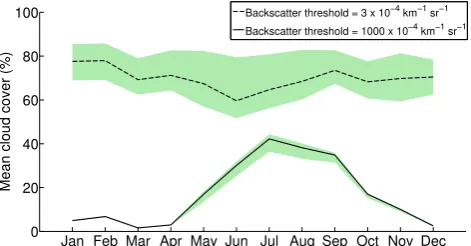
As shown in Fig. 10, there is no apparent seasonal cy-cle at Summit in mean monthly cloud cover when includ-ing the optically thin hydrometeors, with a year-round cloud cover of 72 % (±10 %). This is in contrast with Wang and Key (2005) who found in central Greenland the lowest an-nual mean cloud cover in the Arctic with a value of about 45 %. Such significant difference is probably due to the high amount of very optically thin ice clouds that are easier to be detected by a ground-based ceilometer using a sensitive al-gorithm compared to a satellite product from AVHRR used by Wang and Key (2005). Our results show similar trends to Shupe et al. (2013) who found an overall high cloud occur-rence fraction at Summit combining multiple ground-based instruments. When the optically thin hydrometeors are de-liberately excluded, a seasonal cycle emerges with a summer peak of coverage over 40 % (±4 %), and almost no detections in winter. This agrees with the seasonal distribution of liquid water at Summit (Shupe et al., 2013). These results are influ-enced by the SNR noise reduction that was applied prior to the CBH detection. We assessed the uncertainty in the results due to SNR-threshold choice by varying this threshold from 0.5 to 1.5. The mean introduced uncertainty was 10 % for the low backscatter threshold and 1.5 % for the high backscatter threshold. These uncertainties are also indicated by the green areas in Fig. 10, showing that the overall trends are fairly insensitive to this SNR-threshold choice.
Jan Feb Mar Apr May Jun Jul Aug Sep Oct Nov Dec 0
20 40 60 80 100
Mean cloud cover (%)
Backscatter threshold = 3 x 10⁻⁴km−1sr−1 Backscatter threshold = 1000 x 10−4km−1sr−1
Fig. 10. Monthly mean cloud cover (%) at Summit (2010–2012)
derived with sensitive threshold (3×10⁻⁴km−1sr−1, dashed line) thereby including optically thin hydrometeor layers and higher threshold (1000×10−4km−1sr−1, solid line) thereby focusing on optically thick hydrometeor layers. The green shaded areas repre-sent uncertainty due to SNR-threshold choice.
first 60 m of the profile. We found, however, that 90 % of all profiles with detected hydrometeor layers above 60 m were in fact affected by a significant backscatter signal in the first 60 m. This suggests that at Summit, hydrometeor layers are most frequently present in the first ranges near the surface and can be associated with various phenomena including fog, snowfall and drifting/blowing snow. The CBH distribution of the remaining 10 % after excluding those profiles affected by hydrometeors in the first 60 m indicates that some CBH oc-currences are present higher in the profile (∼1.5 km, green curve in Fig. 11a). Cloud bases of the optically thicker hy-drometeors are still below 1 km (red curve).
At PE, we found a mean cloud occurrence fraction in sum-mer of 46 % (±5 %) for hydrometeor layers with optical depths of at leastτ ∼0.01. When including only optically thicker hydrometeor layers (τ ≥0.5), this fraction reduces to 12 % (±2.5 %). The optically thinnest hydrometeors occur mostly near the surface (35 % of all detections below 500 m, blue curve in Fig. 11b) and progressively less frequently higher in the profiles. Overall 80 % of the CBH values of the detected features is below 2 km, of which the 14 March 2011 case in Fig. 7a is a typical example. Using the high backscat-ter threshold, the resulting CBH detections that are related to optically thicker clouds probably due to supercooled liquid occur mostly (78 %) between 1 km and 3 km (brown curve). Excluding all profiles that are affected by hydrometeors in the first 60 m reduces the cloud occurrence fraction of all detected clouds to 33 %, meaning that 30 % of all profiles containing a hydrometeor layer are affected by near-surface phenomena such as precipitation and blowing/drifting snow. The CBH distribution of the clouds in profiles not affected by these phenomena shows that the optically thin hydrometeor layers are now slightly higher around 500 m (green curve in Fig. 11), while the optically thicker layers are still concen-trated in the 1 to 3 km region (red curve).
Fig. 11. PT CBH occurrence (%) for low (3×10⁻⁴km−1sr−1, blue curves) and high (1000×10−4km−1sr−1, brown curves) thresh-olds. Also shown is CBH occurrence after removing profiles af-fected by hydrometeors in the first 60 m (green and red curves). Un-certainty of the results due to SNR-threshold choice is indicated by the shaded areas. (a) Analysis for Summit (2010–2012). (b) Analy-sis for PE, with data limited to summer months (2010–2013).
Overall, most of the CBH results are situated near the sur-face for both study sites. These findings have important im-plications with regard to other remote sensing instruments that are used to study these areas. For example, satellite sen-sors such as CloudSat carrying an active radar with a blind zone in the lowest ranges due to surface reflection (Marchand et al., 2008) have to take into account that an important part of the hydrometeor layers is situated near the surface.
5 Advantages and limitations of PT algorithm
The PT algorithm is designed to be sensitive to optically thin hydrometeor layers. It has been shown in Sect. 4.3 that the algorithm is successful in detecting such layers. However, as discussed in Sect. 3, the increasing noise levels with height in a ceilometer profile cause the sensitivity of the PT algorithm to decrease with height. This inevitably leads to a decreas-ing amount of detections of the thinnest hydrometeor layers with height. This might imply, for example, that the flat parts of the curves with changing backscatter in Fig. 6 should in reality indicate an increasing amount of detections with de-creasing backscatter. Thin ice clouds high in the atmospheric profile can remain undetected by the PT algorithm. This is however a limitation of the ceilometer that would occur with any method.
Altitude
AGL (km)
σ (km-1)
0 0.1 0.2 0.3 0.4 0.5
0 1 2 3 4 5 6 7
Night Day
Threshold driven SNR driven
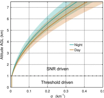
Fig. 12. Extinction profile based on the sensitivity of the PT
algo-rithm for average noise levels during a typical daytime and night-time case. The shaded areas represent uncertainty due to lidar ratio variation between 16 sr< S <25 sr.
the lidar ratioS (Sect. 4.3). Since the PT algorithm is aim-ing at the detection of the first hydrometeor layer in a pro-file, attenuation in the clear polar air below the detection point is negligible, which allows the use of the attenuated backscatterβatt,z as an approximation of the true
backscat-terβz. The backscatter coefficients used for this extinction
profile correspond to the solid orange curve in Fig. 4 that fol-lows the fixed backscatter threshold near the surface and the mean noise level for clear sky higher in the profile. Below the altitude where the PT algorithm uses a fixed backscat-ter threshold (i.e.,±1 km), the sensitivity therefore remains constant (straight parts of the curves in Fig. 12, extinction coefficient ofσ≈0.006 km−1). Above the point where the average noise level exceeds this fixed backscatter threshold, the sensitivity of the PT algorithm becomes dependent on the noise level and hence range. Since the noise level is higher during daytime, when sunlight is scattered into the detector of the ceilometer, the sensitivity of the PT algorithm changes slightly depending on the conditions. We assessed the average noise level with height for typical daytime and night-time profiles at Summit and PE. The extinction pro-files corresponding to these noise levels and therefore to the sensitivity of the algorithm are indicated by the brown (day-time) and blue (night-(day-time) curves in Fig. 12. These curves show a slight variation in the algorithm’s sensitivity from a certain height onwards depending on the conditions (e.g.
σ≈0.155 km−1 to σ≈0.180 km−1 at 5 km AGL), mean-ing that durmean-ing night-time the PT algorithm is slightly more sensitive to optically thin hydrometeor layers compared to daytime. The uncertainty that is introduced by assuming a fixed lidar ratioSis indicated by the shaded areas for which
Swas varied between 16 sr< S <25 sr. This analysis indi-cates the inevitable decrease of some sensitivity of the PT al-gorithm that is related to increasing noise levels with height
in ceilometer backscatter profiles. However, the overall sen-sitivity of the PT algorithm remains very high, meaning that this algorithm is suited for the detection of optically thin hy-drometeor layers as far as detectable by a ceilometer.
6 Conclusions
cloud-base height detection, the robust and relatively low-cost ceilometer can be successfully used to extract informa-tion from various hydrometeor layers over the ice sheets, in-cluding the frequently occurring optically thin ice layers.
Acknowledgements. K. Van Tricht is a research fellow at the
Research Foundation Flanders (FWO). S. Lhermitte was supported in the framework of project GO-OA-25 funded by Netherlands Organisation for Scientific Research (NWO) and as postdoctoral researcher for the FWO. I. V. Gorodetskaya was supported via the project HYDRANT funded by the Belgian Science Policy Office under grant number EN/01/4B, in the frame of which PE measure-ments were performed. J. H. Schween is funded by the Deutsche Forschungsgemeinschaft (DFG) in the transregional collaborative research centre SFB/TR 32. The Summit data were recorded in the frame of the ICECAPS project, which is supported by the US National Science Foundation under grants ARC-0856773, 0904152, and 0856559 as part of the Arctic Observing Network (AON) program, with additional instrumentation provided by the NOAA Earth System Research Laboratory, US Department of Energy ARM Program, and Environment Canada. We are grateful to Christoph Münkel and Reijo Roininen (Vaisala) for continuing support of PE ceilometer and Giovanni Martucci (National Univer-sity of Ireland) for providing the THT code. We would also like to thank the International Polar Foundation for logistical support at PE and Alexander Mangold (RMI) for help with the HYDRANT instrument maintenance. Finally, we would like to sincerely thank the two anonymous reviewers for their constructive remarks.
Edited by: S. Malinowski
References
Barnes, J. E., Bronner, S., Beck, R., and Parikh, N. C.: Boundary Layer Scattering Measurements with a Charge-Coupled Device Camera Lidar, Appl. Optics, 42, 2647, doi:10.1364/AO.42.002647, 2003.
Bennartz, R., Shupe, M. D., Turner, D. D., Walden, V. P., Steffen, K., Cox, C. J., Kulie, M. S., Miller, N. B., and Pettersen, C.: July 2012 Greenland melt extent enhanced by low-level liquid clouds, Nature, 496, 83–86, doi:10.1038/nature12002, 2013.
Bernhard, G.: Version 2 data of the National Science Foundation’s Ultraviolet Radiation Monitoring Network: South Pole, J. Geo-phys. Res., 109, D21207, doi:10.1029/2004JD004937, 2004. Bintanja, R. and Van den Broeke, M. R.: The influence of clouds
on the radiation budget of ice and snow surfaces in Antarc-tica and Greenland in summer, Int. J. Climatol., 16, 1281– 1296, doi:10.1002/(SICI)1097-0088(199611)16:11<1281::AID-JOC83>3.0.CO;2-A, 1996.
Bromwich, D. H., Nicolas, J. P., Hines, K. M., Kay, J. E., Key, E. L., Lazzara, M. A., Lubin, D., McFarquhar, G. M., Gorodet-skaya, I. V., Grosvenor, D. P., Lachlan-Cope, T., and van Lipzig, N. P. M.: Tropospheric clouds in Antarctica, Rev. Geophys., 50, RG1004, doi:10.1029/2011RG000363, 2012.
Campbell, J. R., Hlavka, D. L., Welton, E. J., Flynn, C. J., Turner, D. D., Spinhirne, J. D., Scott, V. S., and Hwang, I. H.: Full-Time, Eye-Safe Cloud and Aerosol Lidar Observation at Atmo-spheric Radiation Measurement Program Sites: Instruments
and Data Processing, J. Atmos. Ocean. Tech., 19, 431–442, doi:10.1175/1520-0426(2002)019<0431:FTESCA>2.0.CO;2, 2002.
Chen, W.-N., Chiang, C.-W., and Nee, J.-B.: Lidar Ratio and Depo-larization Ratio for Cirrus Clouds, Appl. Optics, 41, 6470–6476, doi:10.1364/AO.41.006470, 2002.
Clothiaux, E. E., Mace, G. G., Ackerman, T. P., Kane, T. J., Spinhirne, J. D., and Scott, V. S.: An Automated Algorithm for Detection of Hydrometeor Returns in Micropulse Lidar Data, J. Atmos. Ocean. Tech., 15, 1035–1042, doi:10.1175/1520-0426(1998)015<1035:AAAFDO>2.0.CO;2, 1998.
Curry, J. A., Schramm, J. L., Rossow, W. B., and Ran-dall, D.: Overview of Arctic Cloud and Radiation Char-acteristics, J. Climate, 9, 1731–1764, doi:10.1175/1520-0442(1996)009<1731:OOACAR>2.0.CO;2, 1996.
Curry, J. A., Hobbs, P. V., King, M. D., Randall, D. A., Min-nis, P., Isaac, G. A., Pinto, J. O., Uttal, T., Bucholtz, A., Cripe, D. G., Gerber, H., Fairall, C. W., Garrett, T. J., Hudson, J., Intrieri, J. M., Jakob, C., Jensen, T., Law-son, P., Marcotte, D., Nguyen, L., Pilewskie, P., Rangno, A., Rogers, D. C., Strawbridge, K. B., Valero, F. P. J., Williams, A. G., and Wylie, D.: FIRE Arctic Clouds Exper-iment, B. Am. Meteorol. Soc., 81, 5–30, doi:10.1175/1520-0477(2000)081<0005:FACE>2.3.CO;2, 2000.
Dufresne, J.-L. and Bony, S.: An Assessment of the Primary Sources of Spread of Global Warming Estimates from Cou-pled Atmosphere–Ocean Models, J. Climate, 21, 5135–5144, doi:10.1175/2008JCLI2239.1, 2008.
Ettema, J., van den Broeke, M. R., van Meijgaard, E., van de Berg, W. J., Box, J. E., and Steffen, K.: Climate of the Greenland ice sheet using a high-resolution climate model – Part 1: Evaluation, The Cryosphere, 4, 511–527, doi:10.5194/tc-4-511-2010, 2010. Flynn, C.: Vaisala ceilometer (model CT25K) handbook, ARM
TR-020, available at: http://www.wmo.int/pages/prog/gcos/ documents/gruanmanuals/Z_instruments/vceil_handbook.pdf (last access: 1 March 2014), 2004.
Garrett, T. J. and Zhao, C.: Ground-based remote sensing of thin clouds in the Arctic, Atmos. Meas. Tech., 6, 1227–1243, doi:10.5194/amt-6-1227-2013, 2013.
Gettelman, A., Walden, V. P., Miloshevich, L. M., Roth, W. L., and Halter, B.: Relative humidity over Antarctica from radiosondes, satellites, and a general circulation model, J. Geophys. Res., 111, D09S13, doi:10.1029/2005JD006636, 2006.
Gorodetskaya, I. V., Tremblay, L.-B., Liepert, B., Cane, M. A., and Cullather, R. I.: The Influence of Cloud and Surface Properties on the Arctic Ocean Shortwave Radiation Budget in Coupled Models, J. Climate, 21, 866–882, doi:10.1175/2007JCLI1614.1, 2008.
Gorodetskaya, I. V., Van Lipzig, N. P. M., Van den Broeke, M. R., Mangold, A., Boot, W., and Reijmer, C. H.: Meteorological regimes and accumulation patterns at Utsteinen, Dronning Maud Land, East Antarctica: Analysis of two contrasting years, J. Geo-phys. Res.-Atmos., 118, 1700–1715, doi:10.1002/jgrd.50177, 2013.
Hájek, J., Šidák, Z., and Sen, P.: Theory of rank tests, Aca-demic press, New York, available at: http://www.library.wisc. edu/selectedtocs/bb596.pdf (last access: 1 March 2014), 1967. Heese, B., Flentje, H., Althausen, D., Ansmann, A., and Frey,
S.: Ceilometer lidar comparison: backscatter coefficient retrieval and signal-to-noise ratio determination, Atmos. Meas. Tech., 3, 1763–1770, doi:10.5194/amt-3-1763-2010, 2010.
Heymsfield, A. J. and Platt, C. M. R.: A Parameteriza-tion of the Particle Size Spectrum of Ice Clouds in Terms of the Ambient Temperature and the Ice Water Content, J. Atmos. Sci., 41, 846–855, doi:10.1175/1520-0469(1984)041<0846:APOTPS>2.0.CO;2, 1984.
Hobbs, P. V. and Rangno, A. L.: Microstructures of low and middle-level clouds over the Beaufort Sea, Q. J. Roy. Meteorol. Soc., 124, 2035–2071, doi:10.1002/qj.49712455012, 1998.
Hogan, R. J., Illingworth, A. J., O’Connor, E. J., and PoiaresBap-tista, J. P. V.: Characteristics of mixed-phase clouds. II: A clima-tology from ground-based lidar, Q. J. Roy. Meteorol. Soc., 129, 2117–2134, doi:10.1256/qj.01.209, 2003.
Hov, O. Y., Shepson, P., and Wolff, E.: The chemical composition of the polar atmosphere – the IPY contribution, WMO Bulletin, 56, 263–269, 2007.
Intrieri, J. M.: An annual cycle of Arctic surface cloud forcing at SHEBA, J. Geophys. Res., 107, 8039, doi:10.1029/2000JC000439, 2002.
Jin, X., Hanesiak, J., and Barber, D.: Detecting cloud vertical struc-tures from radiosondes and MODIS over Arctic first-year sea ice, Atmos. Res., 83, 64–76, doi:10.1016/j.atmosres.2006.03.003, 2007.
Kay, J. E. and L’Ecuyer, T.: Observational constraints on Arctic Ocean clouds and radiative fluxes during the early 21st century, J. Geophys. Res.-Atmos., 118, 7219–7236, doi:10.1002/jgrd.50489, 2013.
Kay, J. E., Baker, M., and Hegg, D.: Microphysical and dynamical controls on cirrus cloud optical depth distributions, J. Geophys. Res., 111, D24205, doi:10.1029/2005JD006916, 2006.
King, M. D., Tsay, S. C., Platnick, S. E., Wang, M., and Liou, K.-N.: Cloud retrieval algorithms for MODIS: Optical thick-ness, effective particle radius, and thermodynamic phase, in: Algorithm Theor. Basis Doc. ATBD-MOD-05, NASA Goddard Space Flight Cent., Greenbelt, Md., available at: http://www.modis.whu.edu.cn/chinese/context/info/atmosphere/ atmosphere_optical_mod05.pdf (last access: 1 March 2014), 1998.
Lampert, A., Ström, J., Ritter, C., Neuber, R., Yoon, Y. J., Chae, N. Y., and Shiobara, M.: Inclined lidar observations of bound-ary layer aerosol particles above the Kongsfjord, Svalbard, Acta Geophys., 60, 1287–1307, doi:10.2478/s11600-011-0067-4, 2012.
Lubin, D., Chen, B., Bromwich, D. H., Somerville, R. C. J., Lee, W.-H., and Hines, K. M.: The Impact of Antarctic Cloud Radiative Properties on a GCM Climate Simulation, J. Climate, 11, 447–462, doi:10.1175/1520-0442(1998)011<0447:TIOACR>2.0.CO;2, 1998.
Marchand, R., Mace, G. G., Ackerman, T., and Stephens, G.: Hydrometeor Detection Using Cloudsat – An Earth-Orbiting 94-GHz Cloud Radar, J. Atmos. Ocean. Tech., 25, 519–533, doi:10.1175/2007JTECHA1006.1, 2008.
Martucci, G., Milroy, C., and O’Dowd, C. D.: Detection of Cloud-Base Height Using Jenoptik CHM15K and Vaisala CL31 Ceilometers, J. Atmos. Ocean. Tech., 27, 305–318, doi:10.1175/2009JTECHA1326.1, 2010.
Miloshevich, L. M., Vömel, H., Paukkunen, A., Heymsfield, A. J., and Oltmans, S. J.: Characterization and Correction of Relative Humidity Measurements from Vaisala RS80-A Radiosondes at Cold Temperatures, J. Atmos. Ocean. Tech., 18, 135–156, doi:10.1175/1520-0426(2001)018<0135:CACORH>2.0.CO;2, 2001.
Minnis, P., Yi, Y., Huang, J., and Ayers, K.: Relationships between radiosonde and RUC-2 meteorological conditions and cloud oc-currence determined from ARM data, J. Geophys. Res., 110, D23204, doi:10.1029/2005JD006005, 2005.
Münkel, C., Eresmaa, N., Räsänen, J., and Karppinen, A.: Retrieval of mixing height and dust concentration with lidar ceilometer, Bound.-Lay. Meteorol., 124, 117–128, doi:10.1007/s10546-006-9103-3, 2006.
Murray, F. W.: On the Computation of Saturation Vapor Pres-sure, J. Appl. Meteorol., 6, 203–204, doi:10.1175/1520-0450(1967)006<0203:OTCOSV>2.0.CO;2, 1967.
O’Connor, E. J., Illingworth, A. J., and Hogan, R. J.: A Technique for Autocalibration of Cloud Lidar, J. At-mos. Ocean. Tech., 21, 777–786, doi:10.1175/1520-0426(2004)021<0777:ATFAOC>2.0.CO;2, 2004.
Pattyn, F., Matsuoka, K., and Berte, J.: Glacio-meteorological conditions in the vicinity of the Belgian Princess Elis-abeth Station, Antarctica, Antarct. Sci., 22, 79–85, doi:10.1017/S0954102009990344, 2009.
Pinto, J. O.: Autumnal Mixed-Phase Cloudy Boundary Layers in the Arctic, J. Atmos. Sci., 55, 2016–2038, doi:10.1175/1520-0469(1998)055<2016:AMPCBL>2.0.CO;2, 1998.
Platt, C. M., Young, S. A., Carswell, A. I., Pal, S. R., Mc-Cormick, M. P., Winker, D. M., DelGuasta, M., Stefanutti, L., Eberhard, W. L., Hardesty, M., Flamant, P. H., Valentin, R., Forgan, B., Gimmestad, G. G., Jäger, H., Khmelevtsov, S. S., Kolev, I., Kaprieolev, B., Lu, D.-R., Sassen, K., Shamanaev, V. S., Uchino, O., Mizuno, Y., Wandinger, U., Weitkamp, C., Ansmann, A., and Wooldridge, C.: The Experimental Cloud Lidar Pilot Study (ECLIPS) for Cloud–Radiation Research, B. Am. Meteorol. Soc., 75, 1635–1654, doi:10.1175/1520-0477(1994)075<1635:TECLPS>2.0.CO;2, 1994.
Platt, C. M. R.: Remote Sounding of High Clouds: I. Calculation of Visible and Infrared Optical Properties from Lidar and Radiometer Measurements, J. Appl. Meteorol., 18, 1130–1143, doi:10.1175/1520-0450(1979)018<1130:RSOHCI>2.0.CO;2, 1979.
Pruppacher, H. and Klett, J.: Microphysics of Clouds and Precipi-tation, Vol. 18 of Atmospheric and Oceanographic Sciences Li-brary, Springer Netherlands, Dordrecht, doi:10.1007/978-0-306-48100-0, 2010.
Rowe, P. M., Miloshevich, L. M., Turner, D. D., and Walden, V. P.: Dry Bias in Vaisala RS90 Radiosonde Humidity Pro-files over Antarctica, J. Atmos. Ocean. Tech., 25, 1529–1541, doi:10.1175/2008JTECHA1009.1, 2008.
Sassen, K. and Cho, B. S.: Subvisual-Thin Cirrus Lidar Dataset for Satellite Verification and Climatological Re-search, J. Appl. Meteorol., 31, 1275–1285, doi:10.1175/1520-0450(1992)031<1275:STCLDF>2.0.CO;2, 1992.
Sedlar, J., Tjernström, M., Mauritsen, T., Shupe, M. D., Brooks, I. M., Persson, P. O. G., Birch, C. E., Leck, C., Sirevaag, A., and Nicolaus, M.: A transitioning Arctic surface energy budget: the impacts of solar zenith angle, surface albedo and cloud radia-tive forcing, Clim. Dynam., 37, 1643–1660, doi:10.1007/s00382-010-0937-5, 2010.
Shanklin, J., Moore, C., and Colwell, S.: Meteorological observing and climate in the British Antarctic Territory and South Georgia: Part 2, Weather, 64, 171–177, doi:10.1002/wea.398, 2009. Shupe, M. D. and Intrieri, J. M.: Cloud Radiative Forcing of the
Arctic Surface: The Influence of Cloud Properties, Surface Albedo, and Solar Zenith Angle, J. Climate, 17, 616–628, doi:10.1175/1520-0442(2004)017<0616:CRFOTA>2.0.CO;2, 2004.
Shupe, M. D., Walden, V. P., Eloranta, E., Uttal, T., Campbell, J. R., Starkweather, S. M., and Shiobara, M.: Clouds at Arc-tic Atmospheric Observatories. Part I: Occurrence and Macro-physical Properties, J. Appl. Meteorol. Clim., 50, 626–644, doi:10.1175/2010JAMC2467.1, 2011.
Shupe, M. D., Turner, D. D., Walden, V. P., Bennartz, R., Cadeddu, M. P., Castellani, B. B., Cox, C. J., Hudak, D. R., Kulie, M. S., Miller, N. B., Neely, R. R., Neff, W. D., and Rowe, P. M.: High and Dry: New Observations of Tropospheric and Cloud Proper-ties above the Greenland Ice Sheet, B. Am. Meteorol. Soc., 94, 169–186, doi:10.1175/BAMS-D-11-00249.1, 2013.
Stachlewska, I. S., Piadłowski, M., Migacz, S., Szkop, A., Zieli´nska, A. J., and Swaczyna, P. L.: Ceilometer observations of the bound-ary layer over Warsaw, Poland, Acta Geophys., 60, 1386–1412, doi:10.2478/s11600-012-0054-4, 2012.
Sun, Z. and Shine, K. P.: Parameterization of Ice Cloud Radia-tive Properties and Its Application to the Potential Climatic Importance of Mixed-Phase Clouds, J. Climate, 8, 1874–1888, doi:10.1175/1520-0442(1995)008<1874:POICRP>2.0.CO;2, 1995.
Suortti, T. M., Kivi, R., Kats, A., Yushkov, V., Kämpfer, N., Leiterer, U., Miloshevich, L. M., Neuber, R., Paukkunen, A., Ruppert, P., and Vömel, H.: Tropospheric Comparisons of Vaisala Radioson-des and Balloon-Borne Frost-Point and Lyman-αHygrometers during the LAUTLOS-WAVVAP Experiment, J. Atmos. Ocean. Tech., 25, 149–166, doi:10.1175/2007JTECHA887.1, 2008. Tapakis, R. and Charalambides, A.: Equipment and methodologies
for cloud detection and classification: A review, Sol. Energy, 95, 392–430, doi:10.1016/j.solener.2012.11.015, 2013.
Tselioudis, G., Rossow, W. B., and Rind, D.: Global Pat-terns of Cloud Optical Thickness Variation with Tem-perature, J. Climate, 5, 1484–1495, doi:10.1175/1520-0442(1992)005<1484:GPOCOT>2.0.CO;2, 1992.
Uttal, T., Curry, J. A., Mcphee, M. G., Perovich, D. K., Moritz, R. E., Maslanik, J. A., Guest, P. S., Stern, H. L., Moore, J. A., Turenne, R., Heiberg, A., Serreze, M. C., Wylie, D. P., Pers-son, O. G., PaulPers-son, C. A., Halle, C., MoriPers-son, J. H., Wheeler, P. A., Makshtas, A., Welch, H., Shupe, M. D., Intrieri, J. M., Stamnes, K., Lindsey, R. W., Pinkel, R., Pegau, W. S., Stanton, T. P., and Grenfeld, T. C.: Surface Heat Budget of the Arctic Ocean, B. Am. Meteorol. Soc., 83, 255–275, doi:10.1175/1520-0477(2002)083<0255:SHBOTA>2.3.CO;2, 2002.
Verlinde, J., Harrington, J. Y., Yannuzzi, V. T., Avramov, A., Green-berg, S., Richardson, S. J., Bahrmann, C. P., McFarquhar, G. M., Zhang, G., Johnson, N., Poellot, M. R., Mather, J. H., Turner, D. D., Eloranta, E. W., Tobin, D. C., Holz, R., Zak, B. D., Ivey, M. D., Prenni, A. J., DeMott, P. J., Daniel, J. S., Kok, G. L., Sassen, K., Spangenberg, D., Minnis, P., Tooman, T. P., Shupe, M., Heymsfield, A. J., and Schofield, R.: The Mixed-Phase Arc-tic Cloud Experiment, B. Am. Meteorol. Soc., 88, 205–221, doi:10.1175/BAMS-88-2-205, 2007.
Vömel, H., Selkirk, H., Miloshevich, L., Valverde-Canossa, J., Valdés, J., Kyrö, E., Kivi, R., Stolz, W., Peng, G., and Diaz, J. A.: Radiation Dry Bias of the Vaisala RS92 Humidity Sensor, J. Atmos. Ocean. Tech., 24, 953–963, doi:10.1175/JTECH2019.1, 2007.
Wang, J., Zhang, L., Dai, A., Immler, F., Sommer, M., and Vömel, H.: Radiation Dry Bias Correction of Vaisala RS92 Humidity Data and Its Impacts on Historical Radiosonde Data, J. Atmos. Ocean. Tech., 30, 197–214, doi:10.1175/JTECH-D-12-00113.1, 2013.
Wang, X. and Key, J. R.: Arctic Surface, Cloud, and Radiation Prop-erties Based on the AVHRR Polar Pathfinder Dataset. Part I: Spatial and Temporal Characteristics, J. Climate, 18, 2558–2574, doi:10.1175/JCLI3438.1, 2005.
Wiegner, M. and Geiß, A.: Aerosol profiling with the Jenop-tik ceilometer CHM15kx, Atmos. Meas. Tech., 5, 1953–1964, doi:10.5194/amt-5-1953-2012, 2012.