The Cryosphere, 9, 139–150, 2015 www.the-cryosphere.net/9/139/2015/ doi:10.5194/tc-9-139-2015
© Author(s) 2015. CC Attribution 3.0 License.
Mass changes in Arctic ice caps and glaciers:
implications of regionalizing elevation changes
J. Nilsson1, L. Sandberg Sørensen1, V. R. Barletta1,2, and R. Forsberg1
1Department of Geodynamics, DTU Space, Technical University of Denmark, Elektrovej 327, 2800 Lyngby, Denmark 2Ohio State University, 275 Mendenhall Lab, 125 S. Oval Mall, Columbus, Ohio, 43214, USA
Correspondence to: J. Nilsson ([email protected])
Received: 22 October 2013 – Published in The Cryosphere Discuss.: 11 December 2013 Revised: 27 November 2014 – Accepted: 2 December 2014 – Published: 27 January 2015
Abstract. The mass balance of glaciers and ice caps is sen-sitive to changing climate conditions. The mass changes rived in this study are determined from elevation changes de-rived measured by the Ice, Cloud, and land Elevation Satel-lite (ICESat) for the time period 2003–2009. Four methods, based on interpolation and extrapolation, are used to region-alize these elevation changes to areas without satellite cov-erage. A constant density assumption is then applied to esti-mate the mass change by integrating over the entire glaciated region.
The main purpose of this study is to investigate the sen-sitivity of the regional mass balance of Arctic ice caps and glaciers to different regionalization schemes. The sensitiv-ity analysis is based on studying the spread of mass changes and their associated errors, and the suitability of the dif-ferent regionalization techniques is assessed through cross-validation.
The cross-validation results shows comparable accuracies for all regionalization methods, but the inferred mass change in individual regions, such as Svalbard and Iceland, can vary up to 4 Gt a−1, which exceeds the estimated errors by roughly 50 % for these regions. This study further finds that this spread in mass balance is connected to the magnitude of the elevation change variability. This indicates that care should be taken when choosing a regionalization method, especially for areas which exhibit large variability in elevation change.
1 Introduction
The most recent assessments from the Intergovernmental Panel on Climate Change (Vaughan et al., 2014) and the
Snow, Water, Ice and Permafrost in the Arctic Assessment (AMAP, 2012) state that the mass loss from glaciers and ice sheets is a major contributor to sea-level rise. The use of satellite altimetry to determine the elevation change in the major ice sheets has been possible since the late 1980s and was pioneered by Zwally et al. (1987), Wingham et al. (1998) and others. In recent years this has been expanded to ice caps and glaciers using both satellite and airborne altime-try, in studies such as Gardner et al. (2011), Moholdt et al. (2010a, 2012), Abdalati et al. (2004) and Arendt et al. (2002, 2006).
2 Study areas and data
In this study, we focus on five regions in the Arctic: Iceland (ICEL), Svalbard (SVLB), the Russian High Arctic (RUS), Canadian Arctic North (CAN) and Canadian Arctic South (CAS). The glacier outlines for these areas have been ob-tained from the “Randolph Glacier Inventory” (RGI) (Pfeffer et al., 2014).
The regional mass changes have been estimated from ele-vation changes obtained from the Ice, Cloud, and land Ele-vation Satellite (ICESat) (Schutz et al., 2005) over the time period 2003–2009. ICESat carried the Geoscience Laser Al-timetry System (GLAS), which operated from 2003 to 2009 and had a repeat cycle of 96 days with a 33-day sub-cycle. The system measured the range between the satellite and a surface on the Earth, derived from the delay time between the transmitted laser pulse and the received return echo. The average ground-track sample spacing was 172 m along-track, and the ground footprint was approximately 70 m in diame-ter. The ICESat elevation data are obtained from the National Snow and Ice Data Center (http://nsidc.org/data/icesat/index. html) in the form of the GLA06 L1B global surface elevation data product, product release (R33).
Digital elevation models (DEMs) with a resolution of 1 km (30 arcsec) for use in the elevation-dependent regionalization are available for the five areas. The GTOPO30 DEM is used for the areas of CAS, CAN and RUS. For SVLB and ICEL, DEMs from the National Geospatial-Intelligence Agency (NGA) are used. The GTOPO30 model is estimated to have vertical accuracies of 50–200 m (http://www1.gsi.go.jp/ geowww/globalmap-gsi/gtopo30/gtopo30.html). The NGA DEMs have a similar accuracy, as the data partly have com-mon roots.
To further estimate the quality of the topography mod-els, we have compared them to 2003–2009 surface heights obtained from ICESat by interpolating the DEMs’ surface heights to the ICESat data locations using bilinear interpola-tion. We estimate the standard deviation of the difference be-tween the DEM heights and the ICESat heights to judge their quality. For the GTOPO30 model we find an average stan-dard deviation over all regions of∼65 m and for the NGA DEMs of∼45 m.
3 Data processing
In an initial step, the ICESat GLA06 product has been filtered using the quality flags and rejection parameters included in the product release. Several rejection criteria have been used in the data culling, e.g. data are only used if the flags in-dicated usable elevations (i_ElvuseFlg=1) and only have one peak in the return signal (i_numPk=1). Relevant data (i_satCorrFlg=2) have been corrected with the provided saturation correction. Each elevation measurement has been corrected for the Gaussian centroid (GC) offsets according to
Borsa et al. (2013). There exists an inter-campaign bias in the ICESat data Siegfried et al. (2011) and Hofton et al. (2013), but since this is still debated, we have not applied any bias correction in this study. The RGI glacier outlines have been used to extract only data over the glaciated areas of interest.
The ICESat ground tracks did not have perfect spatial rep-etition, and there could be large (up to 1◦) offsets between the individual tracks from the main ground-track cluster. Tracks with large offsets have been edited out in order to produce more robust elevation change estimates. The ICESat repeat ground tracks are divided into 500 m segments to estimate surface elevation changes. The mean elevation change was estimated in each segment by least-squares regression if data from more than six campaigns were available. This method is described in detail in Sørensen et al. (2011) (referred to in that paper as the M3 method).
A cleaning procedure has been applied to the estimated elevation changes, in which elevation changes with an esti-mated standard deviation (estiesti-mated from the least-squares solution) outside the 95 % confidence interval of the regres-sion errors are removed. Furthermore, a 10-point moving Hampel filter (Pearson et al., 2002) has been used to iden-tify and remove outliers in the elevation changes. The filter-ing is applied in the elevation change versus elevation do-main to ease outlier detection. The success of the screen-ing was judged visually to avoid unnecessary rejection. As a last step, an along-track smoothing filter has been applied to the elevation change data. An unweighted five-point mov-ing average filter with a correspondmov-ing physical filter dis-tance of 2.5 km has been used. Smoothing is undertaken to remove high-frequency noise from the elevation change es-timates, and to aid the fitting procedure for the extrapolation and surface fitting for the interpolation methods, which are described in Sects. 4.2.1 and 4.2.2.
4 Methods
This study uses four different methods that have been imple-mented to regionalize elevation change to partly unmeasured glaciated areas. The four methods can broadly be divided into two categories: interpolation and extrapolation methods. The fundamental difference between the two approaches is what main correlation dependency they use for the regionalization procedure.
J. Nilsson et al.: Mass change in Arctic ice caps and glaciers 141 – M1: smooth surface fit,
– M2: spatial model,
– M3: hypsometric polynomial, – M4: hypsometric elevation bins.
The methods introduced here will be explained in the follow-ing sections.
One of the main sources of uncertainty in the mass change estimation is the conversion to mass via a density assumption (Huss et al., 2013). A constant density of 900 kg m−3is used in this study. This assumption has also been applied by oth-ers, such as Gardner et al. (2011) and Moholdt et al. (2010a, 2012), and has been used in this study to simplify compar-isons to other studies and to ensure that the spread in the mass balance estimates is a result of the different regional-ization schemes alone and not due to the density conversion. 4.1 Regionalization: spatial interpolation
The first regionalization method (referred to as M1) fits a smooth surface to the scattered elevation change estimates, with an along-track resolution of 500 m, using least-squares collocation (as implemented in the GRAVSOFT program GEOGRID; see Forsberg et al., 2008, and Moritz., 1978) onto a regular grid, with a grid spacing of 0.01◦latitude and 0.025◦ longitude, corresponding to a resolution of ∼1 km. The glaciated area of these grids have then been extracted using the RGI glacier outlines.
The least-squares collocation interpolation uses a quadrant-based nearest-neighbour search to find theNq clos-est points in every quadrant around the prediction point. The data points are then interpolated by applying a second-order Markov covariance model. The covariance length is found from the data and the correlation distance is input by the user to the GEOGRID program. The correlation length has been increased until the individual satellite ground tracks are not visible on the surface. This method create a smooth continuous surface between the individual ground tracks, that usually have large cross-track spacing.
Due to data processing and data editing there is a loss of spatial coverage and thus data gaps in the along-track eleva-tion changes. The second regionalizaeleva-tion method (referred to as M2) tries to improve this by re-sampling the along-track data location in every track from 500 to 100 m. This to fill in data gaps and increases the along-track resolution. New along-track elevation changes are then estimated from the en-tire elevation change data set using the following model:
˙
h=a0+a18+a2λ+a3h+. . .+aNhN, (1)
whereh˙ is the parametrized elevation change value,ai are
the model coefficients, h is the DEM elevation, N is the model order, 8 is the latitude andλ is the longitude. The model order used for each region is the same as described
in Sect. 4.1.2 for the spatial extrapolation methods. The M2 approach was chosen because it takes into account the over-all spatial pattern of the elevation changes instead of just the nearest neighbours, which can in some cases be situated far away due to large across-track distances.
For the five regions of interest in this study, the number of points in each quadrant is set toNq=5, and a correlation length of 50 km gave a sufficiently smooth surface.
4.2 Regionalization: hypsometric extrapolation
The third regionalization method (M3) uses hypsometric av-eraging (Nuth et al., 2010; Moholdt et al., 2010a) for ex-trapolation of elevation change estimates to derive volume change. Hypsometric averaging is based on parametrizing elevation changes as a function of elevation using an exter-nal DEM, with the corresponding grid spacing as M1–M2. The glaciated area is divided into elevation bands or bins, and each band is assigned a representative elevation change value, estimated from the parametrized data set.
In M3, the elevation changes are parametrized by fitting a polynomial function to all the elevation change data, as in Nuth et al. (2010) and Moholdt et al. (2010a). The elevations are obtained from the glacier-masked DEMs for every region (see Sect. 2). Hypsometric averaging is then used to extrapo-late the elevation changes regionally.
To determine the degree and the number of terms in the polynomial, we need a measure of how much variance the model is able to account for. The more variability that can be incorporated into the model, the better it will explain the un-derlying statistics of the measured data. We use the adjusted
R2statistics as a measure of incorporated variance (see Mo-holdt et al., 2010a). The degree of the polynomial and the number of parameters are then increased until a convergence of thisR2is reached. For all regions except Svalbard, a lin-ear fit (D=1) was sufficient to parametrize the relation. For Svalbard, a third-order polynomial (D=3) fits the distribu-tion best (as measured byR2, as used by Moholdt et al., 2010a). An elevation bin range of 50 m was chosen for all regions, consistent with Gardner et al. (2011).
The fourth regionalization method (M4) also involves bin-ning the elevation changes according to elevation (as in M3), but instead of estimating the centre bin elevation change from a continuous function we instead use the mean value of the elevation changes inside the bin. Elevation bins that do not contain any data are assigned a value from linear interpola-tion. DEM elevations which are not covered by the ICESat data (usually low and high elevations) are assigned a value from extrapolation of the linear function to these bins, esti-mated from the entire data set.
4.3 Volume and mass change
To determine the regional volume change in the interpolated and extrapolated fields the estimated elevation changes are multiplied by their corresponding area. This procedure dif-fers between the inter and extrapolation methods and is for that reason described below.
To estimate the volume change from the interpolation methods (M1–M2) each individual elevation change grid cell (pixel), hi˙, is multiplied with its corresponding area, corre-sponding pixel areaAp, and summed as follows to obtain the regional volume changeV˙:
˙
V =X(h˙i)·Ap. (2)
The volume change from the extrapolated elevation changes (M3–M4) are estimated in a slightly different way. Here the estimated elevation change for each bin or band is multiplied with the total area of each band, and summed as follows to obtain the regional volume change:
˙
V =X h(z)˙ ·A(z), (3)
whereh˙is the specific elevation change value assigned to the elevation band/binz, which is defined as the centre or mid-elevation of that bin (i.e. 25 m if the bin range is 0–50 m).
A(z)represents the total area inside the elevation band/bin at the specific binned elevationz.
The regional mass change is then estimated by multiply-ing the volume change by a constant density of 900 kg m−3. This approach assumes that the mass changes are due to ef-fects such as ice melt and dynamic thinning while ignoring effects like changes in accumulation rate and firn densifica-tion. This is a very simplified view and is not always valid, which makes it a large source of uncertainty.
Cross-validation
A cross-validation scheme has been employed to assess the quality of the regionalized elevation change fields from the four different methods. As the individual elevation changes are highly correlated along-track, we perform a cross-validation scheme on entire ICESat tracks of elevation changes. The individual ground tracks are assumed to be un-correlated, and the cross-validation is performed in the fol-lowing manner:
1. Remove one of the ground tracks from the original data set.
2. Use M1–M4 to regionalize the elevation changes from the reduced data set.
3. Find the estimated elevation change values from the dif-ferent methods at the locations of the removed ground track.
4. Compute the difference between the estimated and orig-inal elevation changes.
5. Compute the root mean square (rms) of the residuals. 6. Repeat the procedure for all available ground tracks.
This procedure will produce one rms value for each ground track andNrmsfor each method. The mean rms, rms, of all the ground tracks is then used to judge the quality of the dif-ferent regionalization schemes.
5 Error analysis
We base the error analysis on two main concepts – the stan-dard deviation around the mean and the stanstan-dard error of the data – following the approaches of Nuth et al. (2010) and Moholdt et al. (2010a). Several studies have been dedicated to quantifying the individual point measurement errors for ICESat over ice-covered regions. Brenner et al. (2007) found that the ICESat measurement error over ice sheets varied as a function of surface slope, ranging from 0.14 m at 0.1◦up to 0.5 m at 1.2◦. Regions such as Svalbard have a large range in surface slope, varying between 0 and 29◦ at most, with a mean slope of 4.1◦. Therefore, we assume a conservative error ofεicesat= 0.17 m a−1, coming from a measurement er-ror of 1 m (Nuth et al., 2010) and a measurement period of 6 years. This error does not account for the inter-campaign bias present in the ICESat data, which does not affect the spread of the regional mass balance.
To estimate the error from the elevation change estimation procedure, we use the standard deviation estimated from the least-squares solution of the elevation changes as a measure of how trustworthy the individual elevation change measure-ments are (Sørensen et al., 2011). ICESat elevation changes are highly correlated along-track due to distance being short between the measurements, compared to variations in the to-pography. In this study, we have estimated the correlation length from the semi-variogram of the elevation changes, and use the correlation length to spatially bin the eleva-tion changes. The correlaeleva-tion lengths for the five regions are found to be∼15 km for SVLB,∼10 km for ICEL,∼20 km for CAN,∼20 km for CAS and∼10 km for RUS. For more detailed work on this topic, please see Rolstad et al (2009). The bins are then assumed to be uncorrelated, and the total number of non-empty bins is used to estimate the standard error,εdh/dt, for all four methods M1–M4:
εdh/dt = σdh/dt
√
N , (4)
whereN is the number of uncorrelated bins andσdh/dt is
the mean standard deviation of the elevation changes. Here,
σdh/dt has already been reduced by a factor of 1/
√
J. Nilsson et al.: Mass change in Arctic ice caps and glaciers14 Johan Nilsson: Mass change of Arctic ice caps and glaciers: implications of regionalizing elevation changes 143
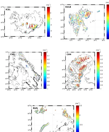
Figure 1: Spatial patterns of elevation changes of the five regions in the form of the satellite ground track coverage. Figure 1. Spatial patterns of elevation changes of the five regions in the form of the satellite ground track coverage.
The least-squares collocation error associated with M1 and M2 is estimated by computing the standard deviation of the data around every prediction point according to Moritz. (1978). The mean value of these standard deviations is used as the interpolation error, and the standard error is computed in the same way as in the elevation change procedure:
εint=
σint √
N, (5)
whereσint is the mean standard deviation from the collo-cation prediction of the data inside the glaciated area.
We quantify the parametrization error from the fitting of the polynomial function used in M2 and M3 by calculating the root-mean-square error (RMSE) between the original
el-evation change estimates and the predicted values:
εfit=
σfit √
N−D, (6)
where σfit is the RMSE between the origi-nal and predicted data, and
√
N−D is the
ad-justment due to the degree of the polynomial. The extrapolation error, εext, relevant for method M3, is quantified by the same approach as used in Nuth et al. (2010), with the extrapolation error being the root-sum-square (RSS) difference of the fitted error minus the elevation change error:
εext=
q
Table 1. The number of error terms present in each method. These
error are then combined into a height error using RSS.
Method Error terms
M1 εicesat,εint,εdh/dt M2 εicesat,εint,εdh/dt,εfit M3 εicesat,εext,εdh/dt M4 εicesat,εb,εdh/dt
The extrapolation error for the mean binning method is re-ferred to as the binning error, εb, not to be confused with
εext. This error is associated with M4 and is defined as the standard deviation inside every elevation bin,σb. The stan-dard error is then calculated by assuming that the individual bins are uncorrelated:
εb=
σb √
N, (8)
The corresponding total elevation change error,εtot, is then estimated as the RSS of the individual error sources as given in Table 1. The volumetric error, εvol, can then be esti-mated by multiplying the elevation change error with the to-tal glaciated area
εvol=εtot·A (9)
We also include an error term,ερ, to account for the simple
density assumption used that ignores the fact that density is actually a function of space and time. The approach follows that of, Moholdt et al. (2010b)
ερ=1
2(ρice−ρfirn), (10)
whereρiceandρfirnare the densities of ice and firn, respec-tively. This error is applied to the entire glaciated region. Finally, we can estimate the mass balance error,εmass, as fol-lows:
εmass=
q
(εvol·ρ)2+(V˙·ερ)2, (11)
whereV˙ is the estimated volume change.
6 Results
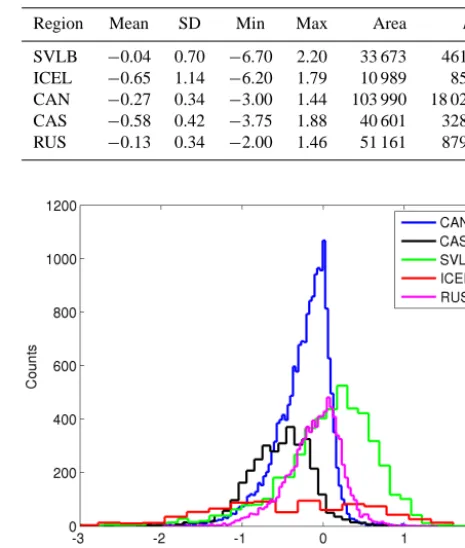
The along-track rates of elevation change have been derived for the five regions: ICEL, SVLB, CAS, CAN and RUS. The elevation change results are shown in Fig. 1. The regions ex-hibit different patterns of rates and variability in the elevation changes. To clarify these differences, a histogram of the el-evation changes for the different regions is shown in Fig. 2, and the associated mean elevation change rate, standard de-viation, and minimum and maximum values are presented in Table 2. ICEL shows the largest mean rate and variabil-ity in elevation change of all five regions, while RUS and
Table 2. ICESat point statistics of elevation change for the different
Arctic regions. The values are in m a−1for the statistics and km2 for the area, andNis the number of observations.
Region Mean SD Min Max Area N
SVLB −0.04 0.70 −6.70 2.20 33 673 4613 ICEL −0.65 1.14 −6.20 1.79 10 989 851 CAN −0.27 0.34 −3.00 1.44 103 990 18 022 CAS −0.58 0.42 −3.75 1.88 40 601 3281 RUS −0.13 0.34 −2.00 1.46 51 161 8797
Figure 2. Histogram of elevation changes for the different Arctic
regions. The Russian High Arctic (RUS) is treated as one region for visualization purposes.
J. Nilsson et al.: Mass change in Arctic ice caps and glaciers 145 et al., 2013). The lower elevations in every region show
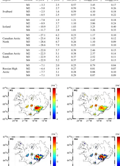
large variability in elevation change, which are clustered around the coastal regions, in areas such as CAN and CAS. Figure 3 shows the elevation change estimates plotted as a function of elevation, together with the estimated DEM hyp-sometry and the ICESat elevations averaged per 50 m eleva-tion bin. Most regions in Fig. 3 show no evident or signifi-cant sampling bias when comparing the ICESat heights and the estimated DEM hypsometry. There are, however, some observed discrepancies in the ICESat sampling for the low elevations in both ICEL and RUS.
The mass changes estimated from all four methods and all five regions in this study are presented in Table 3, which also contains the estimated mass change error and the mean RMSE from the cross-validation procedure for each method. From Table 3 it can be seen that for regions such as CAN, CAS and RUS, only a small spread in their mass balance esti-mates is observed. For these three regions, the spread in mass balance estimates is well within the bounds of the estimated errors. For ICEL and SVLB, the spread of the estimated mass changes from the different methods is on the order of 50 % larger than the estimated mass change errors. The spread of the estimated mass changes for the different regions follows patterns seen in the elevation change variability (Table 2). Regions with high variability such as ICEL and SVLB show a much larger spread in the estimated mass changes than the areas with low elevation change variability.
The validity of the different regionalization schemes has been assessed though a cross-validation setup (Sect. 4.1.3). The results of the cross-validation are presented in Table 3, in the form of the mean, maximum and minimum rms for all four methods and regions. The mean RMSE follows the same pattern as detected in both the mass change estimates and elevation change variability, where areas associated with low elevation change variability and low spread in mass bal-ance, such as CAN, CAS and RUS, show a much lower aver-age rms (∼65 % lower) than ICEL and SVLB. ICEL shows on average the absolute highest RMSE and also the largest spread in rms between the different methods, as much as 20 %. For the other regions, the spread in the RMSE between the different methods show much better agreement, with ob-served differences of up to a few percent. The maximum and minimum values obtained from the cross-validation proce-dure show good agreement for most areas, such as CAN, CAS and RUS. For ICEL and SVLB, a larger spread is ob-served in these two parameters and follows in general the difference in mass balance, at least for SVLB.
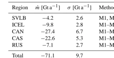
Figure 4 shows the different spatial patterns obtained from the four regionalization procedures for ICEL. Here, the M3 and M4 methods show much larger negative elevation change values at lower elevations than the results based on M1 and M2. The more negative elevation change signal can also be detected in the estimated mass balance for M3 and M4,
which is approximately 26 % more negative than for M1– M2.
7 Discussion
The large degree of variability seen in the lower elevations in Fig. 3 for most regions, especially RUS and CAN, indi-cates that complex spatial and temporal signals have been captured in the data (ice dynamics, ablation, snow accumula-tion, etc.). This variability is clustered into specific coastal areas in regions such as CAN and CAS, where most of the variability is located belowh <500–800 m, and in areas with drainage systems. Most of the more negative elevation changes (h <˙ −1.5 m a−1), on the tail of the elevation change distribution, are also located in these low-elevation areas.
This type of low elevation variability (excluding sampling biases) might help to explain the observed difference be-tween the interpolation and extrapolation methods, seen in Table 3. The extrapolation methods have proven to produce more negative values in these area (h <500–800 m) than the interpolation methods, because the interpolation and extrap-olation regionalization schemes have two fundamental dif-ferences: (i) interpolation methods assume a spatial corre-lation of the elevation changes and (ii) extrapocorre-lation meth-ods assume a vertical correlation in elevation of the elevation changes.
The interpolation approach would in theory (with satisfac-tory spatial coverage) capture the local spatial variability bet-ter than the extrapolation methods, as the extrapolation ods contain no spatial information. The extrapolation meth-ods, on the other hand, make use of the usually high cor-relation to elevation (if the region is homogeneous enough) to produce a model that in principle is more representative of the lower elevations, given no sampling bias, because the interpolation methods might use data further away from the prediction point. These data might be located at higher el-evations or may not be a good representation of the over-all glacier-wide pattern, depending on how far away the data points are.
The main issue to consider for the interpolation methods is the spatial coverage of the data. If the spatial coverage is dense enough, the interpolation will be able to capture the spatial pattern of the region. The main issue to consider for the extrapolation methods is the size of the area used for the parametrization. If the area used for the parametrization is too large, important behaviour of the elevation change pat-tern might not be accounted for in the model. The differences between the interpolation and extrapolation methods can be reduced by dividing the extrapolation region into sub-regions before parametrization, or by including a spatial dependency in the parametrization model.
Figure 3. Elevation change (blue points) as a function of elevation for the different Arctic regions, which are used for the regional
ex-trapolation. The black curve represents the density of ICESat’s sampling and the red curve the DEM hypsometry, both per 50 m elevation bin.
compared to its large size, while ICEL shows a much larger spread in mass balance. This is due to the spatial sampling of the CAN region being dense and the elevation change variability low, compared to ICEL. This has the effect that both the interpolation and extrapolation methods can capture both the spatial and altitudinal patterns of elevation change for CAN, in contrast to, for example, ICEL with its low data density and large variability.
For most areas with a variability lower than 0.45 m a−1 (see Table 2), the impact of the regionalization schemes on the spread of the mass balance is small (on the order of a few percent), with a corresponding spread that falls within the mass balance error. However, for areas with much higher spa-tial variability and magnitude of elevation change, like ICEL
and SVLB, the effect is much more prominent (Table 3). This is most certainly connected to the different types of climate regimes that the regions exhibit. Regions like CAN, CAS and RUS have a continental climate regime (dry and cold), while ICEL and SVLB are in a more maritime climate regime (wet and warm).
J. Nilsson et al.: Mass change in Arctic ice caps and glaciers 147
Table 3. Geodetic mass balancem˙ from the four methods with their corresponding errors (σ), and their mean rms (rms), maximum rms (rmsmax) and minimum rms (rmsmin) from the cross-validation procedure.
Region Method m˙ [Gt a−1] σ [Gt a−1] rms [m a−1] rmsmax[m a−1] rmsmin[m a−1]
M1 −3.3 2.5 0.57 3.45 0.17
M2 −5.0 2.7 0.59 2.76 0.26
Svalbard M3 −2.5 1.6 0.59 4.10 0.18
M4 −0.5 2.5 0.57 4.10 0.22
M1 −7.8 1.9 1.21 4.62 0.18
M2 −8.9 3.7 1.10 3.86 0.24
Iceland M3 −10.9 2.7 1.03 3.25 0.40
M4 −11.7 2.8 1.01 3.26 0.33
M1 −27.1 6.2 0.23 1.17 0.10
Canadian Arctic M2 −25.4 5.8 0.27 1.18 0.12
North M3 −28.6 6.7 0.26 1.10 0.09
M4 −28.6 7.9 0.25 1.03 0.10
M1 −22.0 5.7 0.39 2.46 0.15
Canadian Arctic M2 −22.5 5.1 0.38 2.37 0.14
South M3 −22.9 5.3 0.37 2.52 0.11
M4 −22.9 5.2 0.37 2.47 0.13
M1 −7.1 2.0 0.25 0.79 0.04
Russian High M2 −6.4 1.9 0.27 0.81 0.07
Arctic M3 −7.7 3.1 0.28 0.88 0.10
M4 −7.1 3.9 0.29 0.87 0.09
mass balance for ICEL is−9.8±2.8 Gt a−1 (average of all methods) agrees well with the average contemporary mass loss of−10±1.8 Gt a−1estimated by Björnsson et al. (2013) and Gardner et al. (2013) from glaciological measurements. However, there exists an average difference of roughly 25 % between the interpolation and extrapolation methods, where the average of the interpolation methods −8.35 Gt a−1 is more consistent with the results estimated by Gardner et al. (2013) of−9±2 Gt a−1, while the average of the extrapola-tion methods−11.3 Gt a−1is more consistent with the results estimated by Björnsson et al. (2013) of−11±1.5 Gt a−1.
The difference between the M1–M2 and M3–M4 methods observed in SVLB (Table 3) are most probably due to large spatial variability in the region. The regional parametrization of SVLB might not fully capture the local elevation change pattern as well as the interpolation methods. This effect can be mitigated by applying a spatial dependency, or by dividing the area into sub-regions, as previously discussed. The divi-sion into sub-regions has previously been done by Moholdt et al. (2010a), using the M3 method and a 900 kg m−3 den-sity, yielding a mass balance of−3.7 Gt a−1. This is in good agreement with the estimated mass balance of−4.15 Gt a−1 obtained from this study by averaging the M1–M2 methods. The estimated mass changes for CAS and RUS are on the same order as previous studies. Gardner et al. (2011) found a estimated mass loss for CAS of−24±6 Gt a−1, while Mo-holdt et al. (2012) found a mass loss of −9.8±1.9 Gt a−1 for RUS. Both results are in good agreement with the re-sults obtained from this study of CAS of−22.6±5.3 Gt a−1 and RUS of −7.1±2.7 Gt a−1 by averaging methods M1– M4. The estimated mass balance for CAN, however, shows a much larger difference of roughly 10 Gt a−1compared to Gardner et al. (2011), who also used ICESat. This difference can mostly be explained by the fact that there was no inter-campaign bias included in the elevation change estimation procedure. The exclusion of the inter-campaign bias gave an average mass balance for CAN of roughly−30 Gt a−1. This was further reduced down to−27.4 Gt a−1when the GC set correction (Borsa et al., 2013) was applied. As the GC off-set scales with area, smaller regions are less affected by the offset, while larger regions will show a much larger differ-ence. This is also what is observed in this study when apply-ing the GC offset correction. The size of the mass correction introduced by the trend in the GC offset can be estimated for CAN to roughly 1.9 Gt a−1 by assuming a maximum trend value of 2 cm a−1and the area given in Table 2. This value agrees well with the observed value of roughly 2.6 Gt a−1, which makes the GC offset an important correction for large-scale mass balance studies using ICESat.
To determine whether the 1 km resolution is good enough to give realistic hypsometries, we made a comparison with the ASTER GDEM (http://gdem.ersdac.jspacesystems.or.jp) over Iceland. The ASTER GDEM was re-sampled at a 150 m resolution, to make it easier to handle; binned in 50 m el-evation bands; and plotted against the NGA DEM for
Ice-Table 4. The final regional and total geodetic mass balancem˙ esti-mated using the results from the cross-validation procedure and in situ comparison for Iceland, with corresponding error estimates (σ).
Region m˙ [Gt a−1] σ[Gt a−1] Methods
SVLB −4.2 2.6 M1, M2 ICEL −9.8 2.8 M1–M4 CAN −27.4 6.7 M1–M4 CAS −22.6 5.3 M1–M4 RUS −7.1 2.7 M1–M4
Total −71.1 9.7
land over the glaciated areas. Iceland was chosen because the largest discrepancies between the regionalization methods were found here, and also because it exhibits the largest rate of and variability in elevation change. Even though there ex-ists an apparent sampling bias, the calculated mass changes using the ASTER GDEM (methods M3–M4) gave only a to-tal difference of 2 %. Thus we believe that the 1 km DEMs are of sufficient quality and resolution to give realistic hyp-sometries.
The results of the cross-validation procedure, seen in Ta-ble 3, indicate that, given enough data sampling, the inter-polation and extrainter-polation methods produce regionalized el-evation change estimates of the same quality. Therefore, the interpolation methods described in this study can be used for future mass balance studies in these and other areas even with relatively sparse data sampling. This finding is in contrast to previous discussion, such as that of in Moholdt et al. (2010a), which states that the spatial sampling would usually be to sparse to allow for spatial interpolation, which is definitely true on a sub-regional basis.
J. Nilsson et al.: Mass change in Arctic ice caps and glaciers 149 8 Conclusions
In this study, we have determined the impact of different re-gionalization schemes of elevation changes on the estimated mass balance of five different Arctic regions. These five re-gions consisted of the Canadian Arctic (north and south), the Russian High Arctic, Svalbard and Iceland. The esti-mated mass balance was then, in combination with a cross-validation procedure, used to determine how sensitive these regions are to different regionalization schemes of elevation change. Finally, we also estimated a mass balance budget for each region, using the results derived from the cross-validation procedure and the estimated mass errors.
The study found that the mean rates of and variability in elevation change varied extensively over the different areas in the Arctic. The rate of elevation changes showed a range of 0.6 m a−1across the different regions, while the variabil-ity showed a corresponding range of 0.8 m a−1. Regions with large variability in elevation change showed a large spread in the estimated mass changes from the different methods, given the described setup. This spread was on average 50 % larger than the respective errors. For regions exhibiting low variability, the opposite was observed. Here, the spread of the mass changes lay well inside the estimated errors.
The statistics from the cross-validation procedure, in con-junction with the estimated mass balance results, indicate that the choice of regionalization method for regions with a variability of less than 0.5 m a−1is negligible. However, if the variability exceeds 0.5 m a−1, caution and further anal-ysis is required before choosing a method for mass balance studies. The results from the cross-validation further indicate that the interpolation and extrapolation methods are of the same quality for most areas. Hence the interpolation meth-ods described in this study can also be used for mass balance studies of ice caps and glaciers with satisfactory results.
Acknowledgements. The authors would like to thank the different data contributors: the National Snow and Ice Data Center (NSIDC) for providing the ICESat data; the National Spatial-Intelligence Agency (NGA) for the Svalbard and Iceland DEM; the Ministry of Economy, Trade, and Industry (METI) of Japan and the United States National Aeronautics and Space Administration (NASA) for the ASTER GDEM; and the United States Geological Survey (USGS) for the GTOPO30 DEM. This publication is contribution no. 30 of the Nordic Centre of Excellence SVALI project “Stability and Variations of Arctic Land Ice”, funded by the Nordic Top-level Research. We would like to thank the reviewers, especially Geir Moholdt, for their constructive comments and insights, which greatly improved this manuscript. This work was supported by funding from the ice2sea programme from the European Union 7th Framework Programme, grant number 226375. Ice2sea contribu-tion number 175.
Edited by: E. Hanna
References
Abdalati, W., Krabill, W., Fredrick, E., Manizade, S., Mar-tin, C., Sonntag, J., Swift, R., Thomas, R., Yungel, J., and Koerner, R.: Elevation changes of ice caps in the Cana-dian Arctic Archipelago, J. Geophys. Res., 109, F04007, doi:10.1029/2003JF000045, 2004.
AMAP: Arctic Climate Issues 2011: Changes in Arctic Snow, Wa-ter, Ice and Permafrost, SWIPA 2011 Overview Report, ISBN: 978-82-7971-073-8, 2012.
Arendt, A., Echelmeyer, K., Harrison, W., Lingle, C., and Valentine, V.: Rapid Wastage of Alaska Glaciers and Their Contribution to Rising Sea Level, Science, 297, 382–386, doi:10.1126/science.1072497, 2002.
Arendt, A. A., Echelmeyer, K., Harrison, W., Lingle, C., Zirn-held, S., Valentine, V., Ritchie, B., and Druckenmiller, M.: Updated estimates of glacier volume changes in the western Chugach Mountains, Alaska, and a comparison of regional ex-trapolation methods, J. Geophys. Res.-Earth Surf., 111, F03019, doi:10.1029/2005JF000436, 2006.
Bamber, J., Krabill, W., Raper, V., and Dowdeswell, J.: Anomalous recent growth of part of a large Arctic ice cap: Austfonna, Svalbard, Geophys. Res. Lett., 31, L12402, doi:10.1029/2004GL019667, 2004.
Björnsson, H., Pálsson, F., Gudmundsson, S., Magnússon, E., Adal-geirsdóóttir, G., Jóóhannesson, T., Berthier, E., Sigurdsson, O., and Thorsteinsson, T.: Contribution of Icelandic ice caps to sea level rise: Trends and variability since the Little Ice Age, Geo-phys. Res., 40, 1–5, doi:10.1002/grl.50278, 2013.
Bolch, T., Sandberg Sörensen, L., Simonsen, S. B., Mölg, N., Machguth, H., Rastner, P., and Paul, F.: Mass loss of Green-land’s glaciers and ice caps 2003–2008 revealed from ICE-Sat laser altimetry data, Geophys. Res. Lett., 40, 875–881, doi:10.1002/grl.50270, 2013.
Borsa, A. A., Moholdt, G., Fricker, H. A., and Brunt, K. M.: A range correction for ICESat and its potential impact on ice-sheet mass balance studies, The Cryosphere, 8, 345–357, doi:10.5194/tc-8-345-2014, 2014.
Brenner, A., DiMarzio, J. P., and Zwally, H. J.: Precision and Accu-racy of Satellite Radar and Laser Altimeter Data Over the Con-tinental Ice Sheets, IEEE Trans. Geosci. Remote Sens., 45, 321– 331, doi:10.1109/TGRS.2006.887172, 2007.
Forsberg, R. and Tscherning, C. C.: An overview manual for the GRAVSOFT Geodetic Gravity Field Modelling Programs, avail-able at: http://www.gfy.ku.dk/~cct/publ_cct/cct1936.pdf (last ac-cess: 20 January 2015), 2008.
Gardner, A., Moholdt, G., Wouters, B., Wolken, G., Burgess, D., Sharp, M., Cogley, G., Braun, C., and Labine, C.: Sharply increased mass loss from glaciers and ice caps in the Canadian Arctic Archipelago, Nature, 473, 357–360, doi:10.1038/nature10089, 2011.
Gardner, A., Moholdt, G., Cogley, J. G., Wouters, B., Arendt, A., Wahr, J., Berthier, E., Hock, R., Pfeffer, W. T., Kaser G., Ligten-berg, S. R. M., Bolch, T., Martin, J., Sharp, M. J., Hagen, J. O., van den Broeke, M. R., and Paul, F.: A Reconciled Estimate of Glacier Contributions to Sea Level Rise: 2003 to 2009, Science, 340, 852–857, doi:10.1126/science.1234532, 2013.
li-dar data in East Antarctica, Geophys. Res. Lett., 40, 852–857, doi:10.1002/2013GL057652, 2013.
Huss, M.: Density assumptions for converting geodetic glacier volume change to mass change, The Cryosphere, 7, 877–887, doi:10.5194/tc-7-877-2013, 2013.
Jacob, T., Wahr, J., Pfeffer, W. T., and Swenson, S.: Recent contribu-tions of glaciers and ice caps to sea level rise, LETTER, Nature, 483, 514–518, doi:10.1038/nature10847, 2012.
Kaser, G., Cogley, J., Dyurgerov, M. B., Meier, M. F., and Ohmura, A.: Mass balance of glaciers and ice caps: Consen-sus estimates for 1961–2004, Geophys. Res. Lett., 33, L19501, doi:10.1029/2006GL027511, 2006.
Krabill, W., Abdalati, W., Fredrick E., Manizade, S., Martin, C., Sonntag, J., Swift, R., Thomas, R., Wright, W., and Yungel, J.: Greenland ice sheet: High elevation balance and peripheral thin-ning, Science, 289, 428–430, doi:10.1126/science.289.5478.428, 2000.
Moholdt, G., Nuth, C., Hagen, J. O., Kohler, J.: Recent elevation changes of Svalbard glaciers derived from ICESat laser altimetry, Remote Sens. Environ., 114, 2756–2767, 2010a.
Moholdt, G., Hagen, J. O., Eiken, T., and Schuler, T. V.: Geometric changes and mass balance of the Austfonna ice cap, Svalbard, The Cryosphere, 4, 21–34, doi:10.5194/tc-4-21-2010, 2010. Moholdt, G., Wouters, B., and Gardner, A.: Recent mass change of
glaciers in the Russian High Arctic, Geophys. Res., 39, L10502, doi:10.1029/2012GL051466, 2012.
Moritz, H.: Least Squares Collocation, Reviews of Geophysics and Space Physics, 16, 421–430, doi:10.1029/RG016i003p00421, 1978.
Nuth, C., Moholdt, G., Kohler, J., Hagen, J. O., and Kääb, A.: Svalbard glacier elevation changes and contribution to sea level rise, J. Geophys. Res., 115, F01008, doi:10.1029/2008JF001223, 2010.
Pearson, K. R.: Outliers in process modeling and identifi-cation, IEEE, Transa. Control Syst. Technol., 10, 55–63, doi:10.1109/87.974338, 2002.
Pfeffer, T.W., Arendt, A. A., Bliss, A., Bolch, T., Cogley, J. G., Gardner, A. S., Hagen, J. O., Hock, R., Kaser, G., Kienholz, C., Miles, E. S., Moholdt, G., Mölg, N., Paul, F., Radi´c, V., Rastner, P., Raup, B. H., Rich, J., Sharp, M. J.: The Randolph Consortium, J. Glaciol., 221, 537–552, doi:10.3189/2014jog13j176, 2014.
Pritchard, H. D., Arthern, R. J., Vaughan, D. G., and Edwards, L. A.: Extensive dynamics thinning on the margins of the Greenland and Antartic ice sheets, Nature, 7266, 971–975, doi:10.1038/nature08471, 2009.
Rolstad, C., Haug, T., and Denby, B.: Spatially-integrated geodetic glacier mass balance and its uncertainty based on geostatistical analysis: application to the Western Svartisen ice cap, Norway, J. Glaciol., 55, 666–680, 2009.
Schutz, B. E., Zwally, H. J., Shuman, C. A., Hancock, D., and Di-Marzio, J. P.: Overview of the ICESat Mission, Geophys. Res. Lett., 32, L21S01, doi:10.1029/2005GL024009, 2005.
Siegfried, M. R., Hawley, R. L., and Burkhart, J. F.: High-resolution ground-based GPS measurements show intercampaign bias in ICESat elevation data near summit, Greenland, IEEE, Geosci. Remote Sens., 9, 3393–3400, doi:10.1109/TGRS.2011.2127483, 2011.
Sørensen, L. S., Simonsen, S. B., Nielsen, K., Lucas-Picher, P., Spada, G., Adalgeirsdottir, G., Forsberg, R., and Hvidberg, C. S.: Mass balance of the Greenland ice sheet (2003–2008) from ICE-Sat data – the impact of interpolation, sampling and firn density, The Cryosphere, 5, 173–186, doi:10.5194/tc-5-173-2011, 2011. Vaughan, D. G., Comiso, J. C., Allison, I., Carrasco, J., Kaser,
G., Kwok, R., Mote, P., Murray, T., Paul, F., Ren, J., Rig-not, E., Solomina, O., Steffen, K., and Zhang, T.: Observations: Cryosphere, in: Climate Change 2013: The Physical Science Ba-sis. Contribution of Working Group I to the Fifth Assessment Re-port of the Intergovernmental Panel on Climate Change, edited by: Stocker, T. F., Qin, D., Plattner, G.-K., Tignor, M., Allen, S. K., Boschung, J., Nauels, A., Xia, Y., Bex, V., and Midgley, P. M., Cambridge University Press, Cambridge, UK and New York, NY, USA, 2013.
Wingham, D., Ridout, A., Scharroo, R., Arthern, R., and Shum, C. K.: Antartic elevation change from 1992–1996, Science, 282, 456–4458, doi:10.1126/science.282.5388.456, 1998.