USING ENSEMBLE PRECIPITATION FORECASTS TO IMPROVE HYDROLOGIC RISK
ASSESSMENT AT RIVER CROSSINGS
BY
SEAN ALAN MATUS
THESIS
Submitted in partial fulfillment of the requirements
for the degree of Master of Science in Environmental Engineering in Civil Engineering in the Graduate College of the
University of Illinois at Urbana-Champaign, 2018
Urbana, Illinois
Advisers:
Associate Professor Francina Dominguez Professor Praveen Kumar
ii
ABSTRACT
Current National Weather Service operations forecast hydrologic conditions probabilistically at most of the United States Geological Survey (USGS) stream gauges across the continental United States. The successful implementation of such an approach, operationally, suggests the hypothesis that a probabilistic approach would reduce uncertainty of hydrologic forecasts in ungauged basins. Forecast improvement in ungauged basins is of great interest to the United States Army due to a combination of the remoteness and hydrologic safety risk associated with low-water crossings (LWXs) commonly used as river infrastructure on military training lands. In this work, two historical deadly flooding events were hindcasted at three LWXs at Fort Hood, Texas. A probabilistic precipitation forcing cascades uncertainty through hydrologic and hydraulic models. Each precipitation ensemble member corresponds to an independent model run, resulting in ensembles of streamflow at a 24-hour lead time. The forecast is expanded to predict river hydraulics, through flow velocity and depth, at specific river LWXs. Analysis of the hindcast of two events indicates that cascading probabilistic precipitation through hydrologic and hydraulic models adds robustness to river forecasts compared to deterministic methods. The approach provides a means to communicate the uncertainty of predictions through model member agreement. Analysis of different methods for conveying hydrologic risk from model output leads to our recommendation that a hydraulic safety threshold, calculated as the multiplication of flow velocity and depth, is the best approach for U.S. Army stakeholders in terms of communicating hydrologic risk, as well as associated model uncertainty in the simplest manner possible.
iii
ACKNOWLEDGEMENTS
There are several people whose support made this work possible.
Francina, thank you for being an amazing adviser. You know how to push me when I need to be pushed. You have given me career advice that I carry with me to this day. You motivated me to continue my academic career here.
Praveen, thank you for also being an amazing adviser. Without you, I would not have been able to come study here. You always challenge me to set the bar higher, and you ask the difficult questions that nobody else can ask. From your guidance, I have become a better researcher and student.
Dan, thank you for mentoring me through my graduate career. You are somebody I know I can always turn to for solid advice. I consider you both a mentor and friend. You taught me how to hydro model and showed me the ropes at CERL. One day we will go get those survey points.
Heidi, thank you for employing me at CERL and consequently making all this possible. You somehow convinced me over the phone that packing up my life and moving to Champaign, Illinois was the best move I could make. You were right.
Dad, thank you for supporting me always. You are my hero and I would not be the person I am today without you. You knew how important coming here was for me and pushed me to go, even when you were sick and knew I wanted to say. I love you, Pops.
To the rest of my family and friends, thank you for keeping me sane somehow. My big bro, Scott, thanks for the long vent phone calls. Jacob, Mike, Bry, Fred, Danielle, Div, Cornelia, and so many others, thanks for the memories that made living in the middle of nowhere great.
iv
TABLE OF CONTENTS
CHAPTER 1: INTRODUCTION ... 1
CHAPTER 2: LITERATURE REVIEW ... 6
CHAPTER 3: METHODS ... 12
CHAPTER 4: RESULTS ... 29
CHAPTER 5: DISCUSSION ... 40
CHAPTER 6: CONCLUSION ... 46
REFERENCES ... 48
APPENDIX A: METHODS SUPPORTING INFORMATION ... 56
APPENDIX B: DESIGN STORM SUPPORTING INFORMATION ... 58
1
CHAPTER 1: INTRODUCTION
In June of 2016, nine United States Army soldiers drowned at Fort Hood, Texas when their Light Medium Tactical Vehicle (LMTV) was swept downstream while attempting to cross an at-grade LWX on Owl Creek (Stanglin, 2016). The Investigating Officer stated in the Army Regulation 15-6 executive summary that, “although not directly causing this incident, procedural shortcoming at the installation, company, and platoon levels–specifically, training on local hazards, driver’s training, and LWX hazard reporting – should be improved to more effectively mitigate risks in the future” (US DOD, 2016). In April of 2017, another soldier was killed at Fort Hood when his car was swept away during a flash flood on Turkey Run Creek, and a civilian diver drowned a few days later while looking for the original victim (Myers, 2017).
According to the National Oceanic and Atmospheric Administration (NOAA) National Weather Service’s (NWS) United States Natural Hazard Statistics, flooding related deaths was the second mostly deadly natural hazard of 2017, with 116 victims. This has been consistent for the past 30 years (NOAA NWS, 2018). Texas has been the state with the most flooding (flash and river combined) related deaths for the past 3 years (2015: 48, 2016: 38, 2017: 70). Of those 156 deaths, the NWS reports that 62 involved a vehicle, “likely trying to cross a flooded road” (NOAA NWS, 2016). The NWS encourages the phrase “Turn Around Don’t Drown®” as an educational slogan to remind civilians not to traverse a LWX when there is a clear danger (NOAA NWS, 2018).
The NWS’s educational program notes that, “many of these drownings are preventable.” The 2016 accident was also deemed preventable by the appointed Investigating Officer and ultimately caused by successive decisions of the Vehicle Commander (US DOD, 2016). Fort Hood
2 has multiple warning systems intended to prevent flooding-related accidents. These include NWS flash flood advisories and a LWX status report issued by Fort Hood’s Range Operations (Stanglin, 2016) that specifies which crossings are closed for a given day. There is a network of United States Geological Survey (USGS) water depth gauges across Fort Hood that provide decision support for the LWX status report. Current warnings systems, such as water depth gauges, observe conditions in real time. A dependence on observations limits the current safety measures to only react to conditions that are already occurring. Reactive safety measures have lags between threat recognition and response, thus potentially putting soldiers in danger. In-situ warning systems rely on individual soldiers and leadership making real-time decisions, sometimes without proper training (US DOD, 2016). It has been reported that the LWX report on the morning of June 2, 2016 had the crossings in a “red”, high alert state but this was unbeknownst to those involved in the incident (Stanglin, 2016; US DOD, 2016). Even with the warnings in place, there were “shortcomings” that eventually lead to an individual, in the field, deciding to cross a swollen river which resulted in the loss of his life and eight others.
The tragic accidents, at Fort Hood, bring attention to a need for proactive safety measures. Proactive safety measures, such as road closings based on weather forecasts, anticipate future conditions. The longer lead times associated with predictive safety measures can provide decision makers with the data needed to implement a precautionary response far enough in advance to effectively mitigate hydrologic risk. Military training emulates real-world scenarios and soldiers are trained to be able to make decisions for themselves in the field, but the consequence of a mistake made in training shouldn’t be the loss of life. Proactive safety measures can take the decision to cross a swollen river out of the hands of an individual in the field by giving management
3 level stakeholders the information, and more importantly the time, to make sure that individual is training in a safe manner and can’t make a potentially fatal decision.
Using a combination of forecasting and observation techniques to minimize loss of life and property is the practice of the NWS River Forecast Centers (RFCs). The West Gulf RFC in Fort Worth, TX provides hydrologic predictions, with leads times at a maximum of 5-days, at USGS stream gauges in the Rio Grande (HUC 13) and Texas-Gulf (HUC 12) watershed regions. Of the 336 gauges the WGRFC monitors, 267 have hydrologic forecast capabilities, including those around Fort Hood. The forecasts are driven by Quantitative Precipitation Forecasts (QPFs) from the Weather Prediction Center (WPC). The QPF driven hydrologic forecast for the single USGS streamflow gauge at Fort Hood is noted as using past precipitation and predicted precipitation approximately 12 hours into the future from forecast issuance. A downside to RFC hydrologic predictions is that they are only issued for the USGS gauged basins. To improve hydrologic prediction to ungauged areas, the NOAA Office of Weather Prediction (OWP) has been developing the National Water Model (NWM) through collaboration with the National Center for Atmospheric Research (NCAR). The NWM uses a modeling framework to predict streamflow at every USGS National Hydrography Dataset (NHD) stream across the continental United States. The NWM is driven with High Resolution Rapid Refresh (Benjamin, et al., 2016) and Global Forecasting System (Romine, Schwartz, Synder, Anderson, & Weisman, 2013; Romine, et al., 2014) forecasts for lead times on the orders of hours (HRRR) and days (GFS).
The George E. Box aphorism, “all models are wrong, but some are useful” is at the heart of the theory of using a proactive approach. A proactive, prediction-based approach will almost always have greater uncertainty than observations that occur in real-time, but methods exist to convey that uncertainty effectively. Forecast uncertainty is a result of not just imperfect knowledge
4 of initial conditions, but also from imperfections in the models themselves (Palmer, 2017). The NWM is currently a deterministic model, meaning that a single model run is used to produce a single forecast. The WPC uses a combination of assimilated observations and ensemble forecasts to develop the QPFs, and the QPFs drive the RFC’s hydrologic forecast. Deterministic forecasts provide essentially binary information to decision makers. Action is taken when an event threshold is exceeded in a forecast. A probabilistic forecast uses a collection of model members in an ensemble to convey risk as the probability of an event occurring (Palmer, 2012). The NWS is implementing an operational probabilistic capability for the RFC’s hydrologic forecasts through the Hydrologic Ensemble Prediction Service (HEPS) (Demargne, et al., 2014). Embracing the nonbinary nature of probabilistic forecasting is a simple way for forecasters to convey model uncertainty to decision makers, or “embrace the primacy of doubt” (Palmer, 2017).
In this work, we develop a probabilistic hydrologic forecast that can be used as a decision support tool to minimize flooding safety risks by predicting the probability of necessary crossing closures, 24 hours in advance. Our approach uses an ensemble precipitation forecast to produce an ensemble forecast of streamflow, like the short-term HEPS. The probabilistic character of the streamflow ensemble is a means of conveying prediction uncertainty to stakeholders. The methodology is expanded beyond streamflow prediction to forecast hydraulic conditions at single, ungauged river crossings. Different approaches are evaluated to find a communication strategy of the hydrologic risk information (magnitudes and uncertainties) that can be most effective for decision makers that don’t necessarily have a scientific background. The methodology is tested by hindcasting historical hydrologic events that resulted in loss of life at Fort Hood, TX. The methodology tests the hypothesis that probabilistic precipitation forecasts could be used to reduce the uncertainty of hydrologic risk assessments in ungauged river basins. The objective is that a
5 probabilistic hydrologic framework can be developed to help prevent flooding-related accidents - such as the ones at Fort Hood - from happening again in the future.
6
CHAPTER 2: LITERATURE REVIEW
2.1 Probabilistic Forecasts
At the beginning of the 20th century it was recognized that the laws of physics, represented through a set of prognostic equations, could be used to predict the state of the atmosphere (Abbe, 1901). Numerical weather prediction has since evolved, through theory and technological advances, to benefit society ranging from saving lives to generating substantial financial revenue (Bauer, Thorpe, & Brunet, 2015). Such societal benefits are only possible through an ability to accurately predict weather. The atmosphere is a chaotic system, and as such has finite, state dependent limits of predictability (Lorenz, 1963). Chaotic systems propagate small initial condition perturbations through time leading to eventual forecast and reality divergence (Thompson, 1957). The chaotic unpredictability of weather is the “Achilles Heel” of deterministic weather prediction (Palmer, 2017). A deterministic forecast becomes nothing more than a single “best guess” on a day were the atmosphere is highly unstable. Additional uncertainty is introduced from the observations used for initial conditions and the parameterizations of the equations themselves (Palmer, 2017).
The ensemble prediction system is an alternative to the deterministic approach. In an ensemble system, a collection of forecasts is produced by slightly perturbing model initial conditions and model equations, and then the probability of a weather event is conveyed by the number of ensemble members showing that event (Palmer, 2017). The use of ensemble prediction is rooted in monthly weather forecasting, where timescales were too long for to allow for deterministic prediction. Appearing operationally in the 1980s (Murphy & Palmer, 1986) for extended-range prediction, ensemble weather forecasting is now universal on all timescales (Palmer, 2017).
7 Ensemble Prediction Systems (EPS) are operational at national weather agencies across the globe. The European Centre for Medium-Range Weather Forecasts (ECMWF) EPS is a 10-day forecast with 32 model members (Molteni, Buizza, Palmer, & Petroliagis, 1996). The Weather Prediction Center depends on ensemble forecasts to generate the Quantitative Precipitation Forecasts (QPFs) used to issue weather advisories across the country. Operational short and medium range ensemble forecasts can be publicly downloaded from the National Oceanic and Atmospheric Administration (NOAA) National Operational Model Archive and Distribution System (NOMADS), which was initiated by the National Climatic Data Center (NCDC), National Centers for Environmental Prediction (NCEP), and Geophysical Fluid Dynamics Laboratory (GFDL) (Rutledge, Alpert, & Ebuisaki, 2006).
2.2 Probabilistic Forecasts in Hydrologic Models
In 2017, flooding related deaths was the second mostly deadly natural hazard, with 116. Flooding has consistently been the second most deadly natural hazard, behind heat stroke, for the past 30 years (NOAA NWS, 2018). These statistics would be undoubtedly worse without the NWS implementation of the Advanced Hydrologic Prediction Service (AHPS) nationwide. The AHPS’s operational prediction of streamflow has been valued on the order of billions of U.S. dollars due to its capability to preserve life and property (National Hydrologic Warning Council, 2002). With skillful and timely operational streamflow forecasts being so valuable, there is pressure on forecasting agencies to ensure that the information delivered to water managers and emergency protection services are accurate. The pressure to deliver accurate forecasts is compounded by the fact that hydrologists must work with uncertain datasets and imperfect models. The challenges
8 faced by hydrologic forecasters across the globe can be outlined as four categories (Pagano, et al., 2014):
1. Making the most of available data
2. Making accurate predictions using models
3. Turning hydrometeorological forecasts into effective warnings 4. Administering an operational service
The use of an ensemble hydrologic prediction system is proving to be one of the more effective methodologies to address these challenges (Cloke & Pappenberger, 2009; Zappa, et al., 2010). Hindcast studies have verified these benefits for short and medium range hydrologic forecasts (Bartholmes, Thielen, Ramos, & Gentilini, 2009; Jaun & Ahrens, 2009; Renner, Werner, Rademacher, & Sprokkereef, 2009; Hopson & Webster, 2010; Demargne, et al., 2010; Thirel, Rousset-Regimbeau, Martin, Noilhan, & Habets, 2010; Van Den Bergh & Roulin, 2010; Addor, Jaun, Felix, & Zappa, 2011; Zappa, Fundel, & Jaun, 2013). Starting in 2011, the NWS has been developing and implementing the AHPS Hydrologic Ensemble Forecast Service (HEFS) (Demargne, et al., 2014). The HEFS’s goal is to improve the NWS hydrologic services and quantify the total uncertainty of in streamflow (Wells, 2012). The HEFS is being implemented for the USGS streamflow network, limiting the service to only gauged rivers currently.
2.3 Hydrologic and Hydraulic Modeling
Rainfall-runoff models are the standard for modeling hydrologic processes within a watershed and there are many models that exist to accomplish this developed around the globe, such as the SWAT model (Soil and Water Assessment Tool), MIKE SHE model (Systeme
9 Hydrologique European), HBV model (Hydrologiska Byrans Vattenavdelning model), TOPMODEL, and VIC model (Variable Infiltration Capacity model) (Devi, Ganasri, & Dwarakish, 2015). Deterministic hydrologic models can be classified by complexity as empirical, conceptual, or physics-based (Pechlivanidis, Jackson, McIntyre, & Wheater, 2011). The U.S. Army Corps of Engineers (USACE) has developed its own conceptual hydrologic model, Hydrologic Engineering Center Hydrologic Modeling System (HEC-HMS) (USACE, 2000; USACE, 2016). HEC-HMS has been implemented and verified in a number of modeling studies, being beneficial in its ability to handle different parameterization schemes (spatially represented as a grid or vector) for the physical processes it captures (infiltration, runoff generation, overland flow, channel routing) (Anderson, Chen, Kavvas, & Feldman, 2004; Fleming & Neary, 2004; Knebl, Yang, Hutchison, & Maidment, 2005; Amengual, Romero, Gómez, Martín, & Alonso, 2007; Chu & Steinman, 2009).
To the best of the author’s knowledge, the literature is lacking when it comes to expanding ensemble forecasts beyond hydrologic (streamflow) forecasts at the basin scale, to ensemble hydraulic forecasts (flow velocity and flow depth) at a single river crossing. There is a large suite of hydraulic models available that could be used for this though. The hydraulic modeling of bridges and LWXs can include 1-D, 2-D, and 3-D detail with steady and/or unsteady flow regimes. U.S. Department of Transportation (USDOT) Federal Highway Administration (FHWA) provides an extensive review of the differences between the various types of numerical modeling approaches (USDOT FHWA, 2012). Most bridge hydraulic studies use 1-D analysis methods, though 2-D models are becoming common, and 3-D models are used to analyze complex flow fields. 1-D models are best suited for in-channel flows and when floodplain flows are minor. 1-D models are frequently applicable to small streams and for extreme flood conditions, and generally provide
10 accurate results for narrow to moderate floodplain widths. They can also be used for wide floodplains when the degree of bridge constriction is small, and the floodplain vegetation is not highly variable. In general, where lateral velocities are small 1-D models provide reasonable results. Hydrologic Engineering Center River Analysis System (HEC-RAS) (USACE, 2016; USACE, 2016) is the most widely used 1-D model in the U.S. (USDOT FHWA, 2012). HEC-RAS has been used to model LWXs at a U.S. Army Installation in Indiana (Leahy, 2014). LWXs flow regimes have been modeled at longer time scales to account for a changing climate (Gambill, 2016). HEC-RAS has been evaluated and verified in other modeling studies (Horritt & Bates, 2002; Knebl, Yang, Hutchison, & Maidment, 2005; Hu & Walton, 2008; Moreda, Gutierrez, Reed, & Aschwanden, 2009; Mountz & Crowley, 2009; Wang, 2014). Two-dimensional models should be used when flow patterns are complex and 1-D model assumptions are significantly violated, however, data requirements are much higher. Examples of 2-D models include FST2DH (USDOT FHWA, 2003) and RMA-2 (USACE, 2009).
2.4 Safety Risk at LWXs
“Turning hydrometeorological forecasts into effective warnings” can be considered one of the main challenges for global operational river forecasting agencies (Pagano, et al., 2014). Even if the other three challenges are successfully met by a forecasting agency, the communication with water managers and emergency protection services is essential to preserving life and property.
Safety risk on rivers is not a function of streamflow alone. It is really a function of flow velocity and flow depth. Low velocity & high flow depth conditions can have different safety implications compared to high velocity & low depth conditions, even though both scenarios can have the same streamflow. For this reason, the hydraulic safety threshold has been developed in previous work
11 and applied to both people and vehicles (Affum, Giummarra, & Cheung, 2015). The threshold can protect from the three major causes of deaths at LWXs, listed as (Affum, Giummarra, & Cheung, 2015):
1. A road bed being washed away and/or concealed by floodwaters
2. Stream velocity sweeping a vehicle off the roadway causing the vehicle to roll 3. Stream depth floating vehicles off the roadway
The appropriate value of the hydraulic safety varies in literature, but a general value of 0.40 m2/s has been suggested (Cox, Yee, & Ball, 2004). Empirical and flume studies have been conducted to estimate this value. One study suggests values by vehicle type with 0.30 m2/s for small passenger, 0.45 m2/s for large passenger, and 0.60 m2/s for large 4WD vehicles (Shand, Cox, Blacka, & Smith, 2011). Another study found similar results with a value of 0.35 m2/s for residential vehicles and values ranging 0.35–0.80 m2/s for industrial vehicles (Sutherland, Jones, & Craigie, 1996). VicRoads Road Design Guidelines reports a value of 0.36 m2/s but includes hard limits on flow depth not exceeding 365 mm and recommended not exceeding 200 mm (VicRoads, 2003). Similar hard caps have been specified with a maximum flow depth of 0.5 m regardless of velocity and a maximum velocity of 3 m2/sec at shallow depths (Cox, Shand, & Blacka, 2010).
12
CHAPTER 3: METHODS
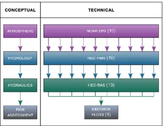
The proposed methodology used a probabilistic precipitation forecast to drive hydrology and hydraulic models, as well as a subsequent river trafficability risk assessment. Each member of the atmospheric ensemble served as boundary condition for the hydrology and hydraulic models, or in other words, each ensemble member ran through the proposed “model chain” in parallel. The “model chain” (Figure 1) began with mesoscale operational weather forecasts. The precipitation from each member of the ensemble weather forecast was used to force its own simulation of basin-scale hydrology in HEC-HMS (USACE, 2000; USACE, 2016). An identical hydrology model was used across simulations. Each member’s timeseries of HEC-HMS streamflow, at the sub-basin scale, was then used to calculate flow velocity and stage at a single river crossing through rating curves generated using HEC-RAS (USACE, 2016; USACE, 2016). The timeseries of flow velocity and stage at a single river crossing were then combined across the separate ensemble members to assess the safety risk at that individual river crossing and the associated uncertainty of the risk.
Figure 1. A schematic of links between data inputs and models. The ensemble weather forecast members are fed in parallel to hydrology and hydraulic models. The ensembles of streamflow, velocity, and stage from the parallel simulations serve as a population sample for analyzing risk assessment.
13 3.1 Precipitation
3.1.1 Ensemble Forecast Selection
The NCAR experimental ensemble prediction system (EPS) was selected as the precipitation forecast for this study (Schwartz, Romine, Sobash, Fossell, & Weisman, 2015). The NCAR EPS has 10-members, 48-hour forecasts initialized daily at 0000 UTC, and a 3-km horizontal grid spacing over the conterminous United States (CONUS). Such characteristics provided a computationally efficient sample size (number of ensemble members) to test the proposed methodology, at a lead time that was considered sufficient for proactive military operational planning, and at a convective-allowing spatial-resolution. Although the NCAR EPS is no longer produced, the experimental High Resolution Rapid Refresh Ensemble (Alexander, et al., 2017) system run at NOAA/ESRL/GSD shares similar characteristics (9-members, 36-hour forecast, and 3-km full CONUS grid) to the NCAR EPS. Eventually, we would use the operational HRRRE version (currently experimental) as a precipitation forecast replacement if the proposed methodology were to be implemented in an operational environment.
3.1.2 NCAR EPS Settings
The NCAR EPS consists of analysis and forecast components. The forecast model component is the Weather Research and Forecasting Model (Skamarock, et al., 2008). The analysis model component is the Data Assimilation Research Testbed (Anderson J. L., 2009) software, and more specifically an ensemble adjustment Kalman filter (Anderson J. L., 2001; Anderson J. L., 2003) within the software. The EAKF analysis provides initial conditions (ICs) for the WRF forecasting.
The NCAR EPS is a single-physics system, thus each ensemble member uses an identical physics and dynamics configuration. Refer to journal paper for specific configuration details
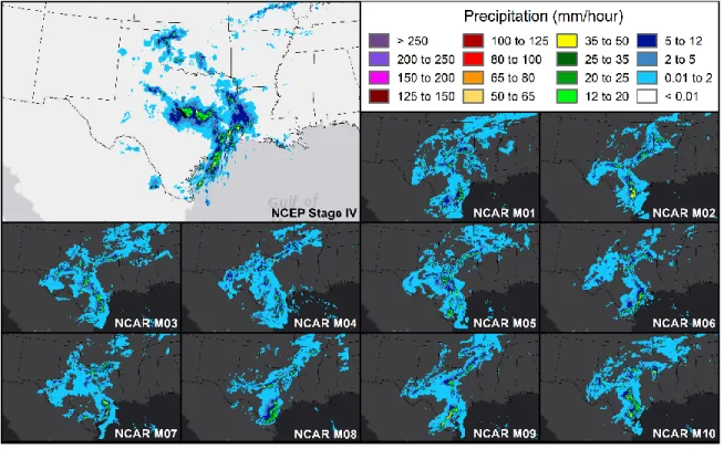
14 (Schwartz, Romine, Sobash, Fossell, & Weisman, 2015). Lateral boundary conditions (LBCs) are derived from perturbing GFS forecasts at 3-hour intervals. The 15-km EAKF analysis ICs and the 15-km GFS perturbed LBCs are interpolated to the nested domain 3-km grid. Figure 2 is an example of the publicly available NCAR EPS product with precipitation rates shown for the same timestep across ensemble members and compared to NCEP Stage IV observations on June 2, 2016 1400–1500 UTC.
Figure 2. Example precipitation output from the NCAR EPS members (black background plots) and NCEP Stage IV observations (top left grey background plot) for the same hour. It can be seen how an identical model physics and dynamics configuration, but perturbed LBCs and ICs can generate different precipitation fields across ensemble members on June 2, 2016 14:00–15:00 UTC.
3.1.3 Precipitation Preprocessing
The NCAR EPS precipitation data is publicly available for download in the General Regularly-distributed Information in Binary (GRIB) format. The data is at 3-km resolution and projected in the Polar Stereographic coordinate system. The precipitation was preprocessed
15 temporally by extracting the first 24-hours of the full 48-hour forecast for each daily initialization. The extraction generated a timeseries of precipitation without overlapping timesteps.
The preprocessing converted the precipitation to a Digital Speech Standard (DSS) file format (USACE, 2009; USACE, 2011) that could be ingested into the hydrology model used. The precipitation was projected into the Albers Equal-Area coordinate system. Additionally, the precipitation was regridded from a 3-km resolution to a 1-km resolution through bilinear interpolation. The interpolation was necessary because the hydrology model used in this study only accepts gridded forcing in an equal area projection at 2-km, 1-km, or 500-m spatial resolution. The 1-km grid was selected because it was the coarsest option that was a factor of 3 (subdivides grid cells cleanly). Figure 10 is an example of preprocessed precipitation for a single forecast hour.
3.2 Hydrology: HEC-HMS
The precipitation ensemble members were used as boundary conditions for the basin-scale hydrology model. The model transforms excess precipitation into runoff. The model was built with the HEC-HMS software. HEC-HMS model outputs streamflow hydrographs at each reach within the defined basin.
3.2.1 Study Site
Cowhouse Creek was selected for the hydrologic modeling in this study. Cowhouse Creek has 7 LWXs on its main channel, which are within Fort Hood’s training lands. The basin is also minimally gauged, with only a single USGS streamgauge. The corresponding basin is USGS HUC (Hydrologic Unit Code) 12070202 and is herein referred to as the Cowhouse Creek catchment.
16 The Cowhouse Creek catchment is located in central Texas (bounding coordinates: 31°44’
N, 97°46’ W, 31°04’ N, 98°35’ W). The 1625 km2 catchment has contributing drainage area spanning Bell, Coryell, Hamilton, Lampasas, and Mills counties. The catchment is mostly open rangeland (74% grassland/shrub/pasture) and undeveloped (5% developed) (MRLC Consortium, 2011). The catchment has silty and clayey soils (Sand: 23%, Silt: 42%, Clay: 35%) and high runoff potential based on the hydrologic soil groups (HSGs) (A: 0%, B: 13%, C: 38%, D: 49%) (USDA NRCS, 2010; USDA NRCS, 2018).
3.2.2 Watershed Delineation
The Cowhouse Creek catchment was delineated from the USGS National Elevation Dataset (NED), which has a 10-m horizontal and 1-m vertical resolution for the region. The Arc Hydro and HEC-HMS preprocessing toolboxes were used within the ArcGIS software suite developed by Environmental Systems Research Institute (ESRI) to delineate the catchment and stream network. The delineated watershed is shown in Figure 3 with the Cowhouse Creek catchment, sub-basins, and stream network.
Figure 3. Watershed and stream network delineation produced using the NED 10-m DEM and the Arc Hydro Toolbox within ArcGIS for the Cowhouse Creek catchment.
17 The NED Digital Elevation Model (DEM) was preprocessed by applying a fill filter to force all flow to accumulate at the catchment pour point. The network was delineated by chaining the generic subroutines within the Arc Hydro toolbox. A value of 10-km2 (108,515 grid cells) was used as the minimum contributing area to initiate a stream within the Stream Definition subroutine. The value is user-defined but was validated by comparing the stream network delineated visually to the Cowhouse Creek stream network in the USGS National Hydrography Dataset (NHD).
3.2.3 HEC-HMS Model Configuration
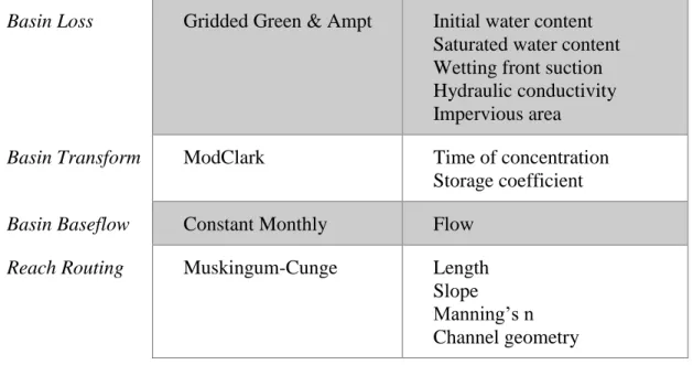
HEC-HMS is used to calculate the excess precipitation over the catchment, then to route that excess precipitation as runoff over the sub-basins and through the catchment river/creek reaches. The model configuration selected to capture this physical process is shown in Table 1. The following describes each of these processes in detail.
Table 1. HEC-HMS configuration used and method parameters that must be user specified.
Process Method Parameters
Basin Loss Gridded Green & Ampt Initial water content Saturated water content Wetting front suction Hydraulic conductivity Impervious area
Basin Transform ModClark Time of concentration
Storage coefficient
Basin Baseflow Constant Monthly Flow
Reach Routing Muskingum-Cunge Length
Slope Manning’s n Channel geometry
18 3.2.3.1 Gridded Green and Ampt Loss Method
The basin loss module of HEC-HMS models infiltration of precipitation into the soil. The gridded Green and Ampt Loss method (Mein & Larson, 1973) was selected for this study. A gridded method was preferred because the infiltration grid could be matched to the grid of the NCAR EPS precipitation. The Green and Ampt Loss method was selected because the necessary parameters can be estimated from soil information. Such a method is preferred in ungauged catchments, such as the Cowhouse Creek catchment with its single USGS streamflow gauge.
The Green and Ampt infiltration method is an event-based (does not consider processes significant at longer temporal scales, such as evapotranspiration), distributed (spatial variability is explicitly considered), conceptual (physically based rather than empirical), and fitted-parameter model (includes parameters that cannot be physically measured) (USACE, 2000). The method assumes the same initial conditions and simple soil model as the Richards’ equation, as well as a uniform, infinitely deep soil column and a user-defined initial water content (USACE, 1994). The method computes infiltration over pervious areas, as specified in the HEC-HMS Technical Manual (USACE, 2000): ft = K [1 + (ϕ − θi)Sf Ft ] (1) Where: ft= K = (ϕ − θi) = Sf= Ft=
Loss during period, t
Saturated hydraulic conductivity Volume moisture deficit (Soil porosity less the initial water content)
Wetting front suction
Cumulative loss during period, t
Grids of saturated water content, hydraulic conductivity, wetting front suction, initial water content, and impervious area are specified as inputs in HEC-HMS.
19 Saturated water content, hydraulic conductivity, wetting front suction grids were generated using United States Department of Agriculture (USDA) Natural Resources Conservation Service (NRCS) Soil Survey Geographic Database (SSURGO) vector data (USDA NRCS, 2018) and the USDA Agricultural Research Service (ARS) ROSETTA hydraulic parameter model (Schaap, Leij, & van Genuchten, 2001). The variables sand/silt/clay percentage, bulk density at 15-bar, and water content percentage at 15- and 33-bar were extracted from the SSURGO database using the USDA NRCS Soil Data Viewer (ArcGIS plug-in tool). The variables were aggregated in the vertical through a weighted average across the soil column to produce a 2-D vector layer. The vectors of each soil variable were interpolated to the same 1-km horizontal grid as the NCAR EPS precipitation, through a zonal average. The soil 1-km grids were then exported from ArcGIS to an ASCII file format to be imported into the ROSETTA hydraulic parameter estimation computer program (Schaap, Leij, & van Genuchten, 2001). ROSETTA uses a hierarchal artificial neural network (ANN) combined with the bootstrap method to calculate hydraulic parameters through pedotransfer functions. Output from ROSETTA consists of the van Genuchten water retention parameters α and n (van Genuchten, 1980), residual water content, saturated water content, hydraulic conductivity (For ROSETTA graphic user interface, see Figure 11).
The wetting front suction grid was estimated from the ROSETTA output and the van Genuchten formulation for pressure head at the P-point on the soil-water retention curve (van Genuchten, 1980). The P-point is located halfway between the residual, θr, and saturated, θs, water contents. Although this is an approximation, water front suction values ranged from 3.0–58 cm which matched well to those suggested in literature (Sand: 10.6 cm, Silt loam: 40.4 cm, Clay: 71.4 cm) (Rawls, Brakensiek, & Miller, 1983). The formulation for pressure head at the P-point is taken from (van Genuchten, 1980):
20 hp =1 α[2 1/m− 1]1−m (2) m = 1 − 1/n (3) Where:
α, m, n = Soil specific parameters estimated from ROSETTA
HEC-HMS could not be run in a continuous mode with the Green and Ampt configuration because this loss method does not account for evapotranspiration, which becomes significant at longer time scales. Consequently, the initial water content grid was estimated as the top 10-cm soil moisture simulated from the mosaic land-surface model for Phase 2 of the North America Land Data Assimilation System (NCEP EMC, 2009; Xia, et al., 2012). Two initial water content grids were generated with hourly NLDAS-2 soil moisture data for the first timestep of each simulation (March 26, 2017 00:00 UTC and May 17, 2016 00:00 UTC). The NLDAS-2 data were regridded in the same manner as the NCAR EPS precipitation to match the other soil parameter grids.
Lastly, the impervious area grid came directly from the National Land Cover Database (NLCD) 2011 percent developed imperviousness dataset (MRLC Consortium, 2011) and was zonally averaged to the same grid as the other parameters.
3.2.3.2 ModClark Excess Precipitation Transform Method
The transform method in HEC-HMS calculates the time elapsed between the time precipitation becomes excess at the soil surface and contributes to a stream reach as runoff. The HEC-HMS modeling package requires the ModClark transform method be used when a gridded loss method is selected. The ModClark method requires two parameters: time of concentration and storage coefficient.
21 The time of concentration was estimated using the SCS watershed lag method (Mockus, 1961; USDA NRCS, 2010). The watershed lag method formulation (Equations 4-7) required flow length, converted to Imperial units, and catchment slope which were both calculated using HEC-GeoHMS (USACE, 2013). The curve number was also required and taken from tables in USDA NRCS Technical Reference #55 that correlated curve number to NLCD land cover type (USDA NRCS, 1986). The storage coefficient was assumed to be equal to the maximum potential retention, from the watershed lag formulation (Mockus, 1961), as it is in additional literature (Simas, 1996; USDA NRCS, 2010). It is understood that this assumption is weak, because it is based off an assumption in a study that generated empirical equations and ignored units as a result (Simas, 1996). For this reason, the ModClark storage coefficient is reserved to be used as a calibration parameter if needed.
L =(l) 0.8(S + 1)0.7 1900Y0.5 (4) L = 0.6 Tc (5) S = 1000 cn′ − 10 (6) cn′= CN (7) Where: L = Tc = l = Y = S = cn′ = CN = Lag (hr) Time of concentration (hr) Flow length (ft)
Average watershed land slope (%) Maximum potential retention (in) Retardance factor
22 3.2.3.3 Constant Monthly Baseflow Separation Method
Baseflow was calculated as a constant monthly value. The historical record of daily streamflow covering 1950-2018 was digital filtered (Lyne & Hollick, 1979) with a filter parameter of 0.925 recommended by literature (Nathan & McMahon, 1990) (see Figure 12 for timeseries). The baseflow calculated from the filter was only accurate for the sub-basin that included the USGS gauge observations. The baseflow magnitudes in other sub-basins were estimated as the baseflow calculated in the USGS gauge sub-basin multiplied by the ratio of the area of the sub-basin in question to the sub-basin that contained the USGS gauge.
3.2.3.4 Muskingum-Cunge Routing Method
The Muskingum-Cunge model was selected as the routing method within the HEC-HMS hydrologic model. The method was selected because of its applicability in basins that are difficult to calibrate due to the lack of hydrograph observations and because of the gradually sloped channels in the Cowhouse Creek catchment. The Muskingum-Cunge method solves a form of the Saint Venant equations where the continuity equation allows for lateral inflow and the momentum equation takes the diffusive form, assuming the acceleration terms are negligible.
∂A ∂t + ∂Q ∂x = qL (8) gA∂y ∂x− gA(S0− Sf) = 0 (9) Where: Q = A = x, t = qL= g = y = Flow Cross-sectional area
Spatial and temporal discretization Lateral inflow
Gravitational constant Water depth
23 S0 =
Sf=
Channel slope Friction slope
The Muskingum-Cunge method combines these forms of the Saint Venant equations with a linear approximation to produce the convective diffusion equation (Miller & Cunge, 1975).
∂Q ∂t + c ∂Q ∂x = μ ∂2Q ∂x2 + qL (10) c = dQ dA (11) μ = Q 2BS0 (12) Where: c = μ = B = Wave celerity Hydraulic diffusivity Top width of water surface
When combined with the Muskingum finite difference approximation of the continuity equation, the final formulation that HEC-HMS solves for the Muskingum-Cunge routing method is (USACE, 2000): Ot = C1It−1+ C2It+ C3Ot−1+ C4(qLΔx) (13) C1 = Δt K + 2X Δt K + 2(1 − X) (14) C2 = Δt K − 2X Δt K + 2(1 − X) (15) C3 = 2(1 − X) −ΔtK Δt K + 2(1 − X) (16) C4 = 2 ( Δt K ) Δt K + 2(1 − X) (17) K =Δx c (18) X = 1 2(1 − Q BS0cΔx) (19)
The routing method is solved with an explicit numerical scheme. As such, the model is at risk of becoming numerically instable if the spatial and temporal discretizations aren’t at small enough
24 resolutions. For this reason, the automatic adaption time interval method within HEC-HMS was used for this study. The automatic adaption allowed for variable time intervals to be used to route flow through the channel. The variable numerical timestep helped minimize instances where the model did not converge.
Specified channel parameters for this method included length, slope, Manning’s n and geometric shape. Channel length and slope were calculated in ArcGIS with the HEC-GeoHMS preprocessing tools (USACE, 2013). Channel Manning’s n was determined to be 0.04 from comparing photographs taken in the field (see Cowhouse Creek Channel in Appendix C for photographs) to reference tables (Chow, 1959). Channel geometric shape was estimated as an 8-point representative cross-section. Only one cross-section could be specified per sub-basin. A section was digitized every 500 meters using ArcGIS and then averaged across all cross-sections for an individual sub-basin (see Figure 13 for example).
3.3 Hydraulics: HEC-RAS
HEC-HMS provides timeseries of streamflow per stream reach, however, this study requires time-varying flow velocity and depth at a single stream crossing. To do so, hydraulic rating curves were created for three different LWX structures on Cowhouse Creek. A hydraulic model for a single reach on Cowhouse Creek was built and run with HEC-RAS. The model spatial features were digitized in ArcGIS with the HEC-GeoRAS toolbox (USACE, 2011). The stream channel was imported from the HEC-HMS model. Stream banks and stream flow paths were digitized by hand using aerial images and the terrain DEM. Cross-sectional cut lines were digitized every 250-meters (see Figure 14 for HEC-RAS model domain and digitized features). The improved ford LWXs were modeled as inline broad-crested weirs (see LWX #15 and LWX #16
25 in Appendix C for photographs). The vented ford LWX was modeled as a series of pipe arch shaped culverts with an embanked roadbed on top (see Jackson Crossing in Appendix C for photograph). Structure geometries and elevations were determined from point survey data collected from multiple field trips to the basin.
User specified parameters included Manning’s n values for the channel (0.040) and over the channel banks (0.045). These parameters were selected from the comparison of field photographs to values in HEC-RAS’s Reference Manual Table 3-2 (USACE, 2016). Flow contraction and expansion parameters were taken from HEC-RAS’s Reference Manual Table 3-3 as 0.1 and 0.3 respectively for unvented crossings. Parameter values of 0.3 and 0.5 were used for the vented crossing based on previous work (Gambill, 2016).
Structure rating curves were generated by running the HEC-RAS model successive times with a steady-state, subcritical flow regime. The initial conditions were an upstream flow hydrograph ranging from 1–1000 m3s-1 and a downstream boundary condition assumed to be the normal flow depth. The HEC-RAS software computes the water surface profile from one model cross-section to the next by solving the Energy equation with the assumptions that the flow is steady-state, and gradually varying (USACE, 2016; USACE, 2016).
Z2+ Y2+ a2V22 2g = Z1+ Y1+ a1V12 2g + he (20) he = LS̅ + C |f a2V22 2g − a1V12 2g | (21)
L =LlobQ̅lob+ LchQ̅ch+ LrobQ̅rob Q̅lob+ Q̅ch+ Q̅rob
(22) Where:
26 Y1, Y2 = V1, V2 = a1, a2 = g = he = L = S̅ =f C = Llob, Lch, Lrob= Q̅lob, Q̅ch, Q̅rob=
Depth of water at cross sections Average velocities
Velocity weighting coefficients Gravitational acceleration Energy head loss
Discharge weighted reach length Representative friction slope
Expansion/Contraction loss coefficient Cross-sectional reach lengths
Arithmetic average of the flows between sections
Once the rating curves were developed from running 1000 HEC-RAS simulations with varying initial condition magnitude, the output from HEC-HMS could be converted from discharge to velocity and depth using the rating curves. For this study HEC-RAS was only used to generate the hydraulic rating curves at each LWX structure.
3.4 Risk Assessment
Three separate methods were investigated as ways to assess risk from the model outputs. The methods use the output from HEC-HMS and the rating curves from HEC-RAS. The goal is to communicate the hydrologic risk, as well as the uncertainty of that hydrologic risk to stakeholders.
3.4.1 Flow-Duration Curve
The first approach generated the flow-duration curve for Cowhouse Creek from the USGS gauge observations (USGS, 2016). The flow-duration curve is an empirical cumulative distribution function that describes the percentage of time over the entire record that daily streamflow equals or exceeds some specified value (Maidment, 1993). Using R (Zeileis & Grothendieck, 2005; R Core Team, 2017; Fuka, Walter, Archibald, Steenhuis, & Easton, 2018), the flow-duration curve was calculated as the exceedance probability of each ranked daily flow value for the period of record (Zambrano-Bigiarini, 2017).
27 P = 100 M n + 1 (23) Where: P = M = n = Exceedance probability
Flow rank (1: Largest daily flow) Number of daily flow values
The average daily streamflow for the two days when there was loss of life (April 3, 2017 and June 2, 2016) was then calculated for each streamflow ensemble member and overlaid on the flow-duration curve. To convey ensemble member agreement, a heatmap was also plotted as part of the figure that showed model member agreement by grouping by streamflow order of magnitude.
3.4.2 Return Period
The second approach used flood frequency analysis to better isolate the extremes in the hourly data and without averaging to a daily time scale. The flood frequency analysis in this study used the return period metric, which measures the average interval between events equaling or exceeding a probability threshold. Return period analysis assumes that flood events are assumed to be independent and identically distributed.
The historical peak streamflow observations were used from the USGS gauge on Cowhouse Creek. The annual peak streamflow observation is the maximum instantaneous observation recorded at the gauge every year. To calculate return periods, the population of annual peak streamflow was assumed to follow a log-normal distribution (Delignette-Muller & Dutang, 2015). That assumption was then investigated for statistical significance with the Sharpiro-Wilk (Royston, 1982) and Lilliefors (Dallal & Wilkinson, 1986) goodness-of-fit tests with an alpha value of 0.05 (Gross & Ligges, 2015). Once a distribution to characterize the peak flow population was established, the return period for the maximum streamflow simulated for each ensemble model
28 member was calculated as the inverse of the exceedance probability from the fitted distribution. The exceedance probability was calculated using the plnorm function from the stats package within R (R Core Team, 2017).
3.4.3 Safety Threshold
The third risk assessment approach was utilized to expand the risk assessment of streamflow, to the assessment of flow velocity and depth. Such an approach was deemed necessary because dangerous hydrologic scenarios can occur under flow conditions of low velocity, but high depth and vice versa. The safety criterion for vehicles crossing a river structure used in this study is the product of water depth and depth of flow (Affum, Giummarra, & Cheung, 2015). An arbitrary value of 0.4 m2/s was selected for this study based on previous values from the literature (Sutherland, Jones, & Craigie, 1996; VicRoads, 2003; Cox, Yee, & Ball, 2004; Cox, Shand, & Blacka, 2010; Shand, Cox, Blacka, & Smith, 2011).
A risk assessment figure was generated by calculating the safety criterion hourly for each ensemble member of flow velocity and depth and comparing those calculations to the threshold value of 0.4 m2/s. Hydrologic risk uncertainty was depicted as the number of ensemble members that exceed the safety threshold.
29
CHAPTER 4: RESULTS
We use the methodology described in Chapter 3 to hindcast two hydrologic events that resulted in loss of life at Fort Hood, Texas. These events occurred on April 3, 2017 and June 2, 2016. The hindcasts are for three LWXs along Cowhouse Creek.
4.1 Precipitation Characteristics
The preprocessed NCAR 3 km, 10-member Ensemble is used as the atmospheric forcing to hindcast the two hydrologic events with a 24-hour lead time. The variability of accumulated precipitation across ensemble members is shown in Figure 4 for the two events. The ensemble means of accumulated precipitation that led to the two deadly accidents are 49.8 mm (04/02/17) and 110.9 mm (05/29/16–06/01/16). The maximum precipitation rate for the ensemble means are 13.6 mm/hour (2017) and 6.6 mm/hour (2016).
It can be seen in Figure 4 that both events were preceded by a separate precipitation event. During 03/28/17–03/29/17, the accumulated precipitation averaged over ensemble members is 13.0 mm. In 2016, this value is 67.6 mm over the 5 days, 05/17/16–05/21/16.
The spatially weighted average 100-year design storm for a 1-hour duration, determined from regional frequency analysis with the L-moment method with local rain gauge observations is 89 mm/hour (see Appendix B for details). The maximum precipitation rates of 13.6 mm/hour and 6.6 mm/hour equate to design storms with return periods of 0.3 and 0.2 years.
30
Figure 4. Box and whisker plots of daily accumulated precipitation averaged spatially for the area upstream of the USGS streamflow gauge on Cowhouse Creek. Each sample consists of the 10 members from the NCAR Ensemble showing the spatial variability across the ensemble members. The 2017 event (top plot) shows less variability across precipitation members for a smaller event compared to the larger 2016 event (bottom plot)
4.2 Hydrology and Hydraulics
4.2.1 Hydrologic Response
We obtain a 10-member streamflow ensemble for each event by running the Cowhouse Creek HEC-HMS model separately for each member of the NCAR ensemble. The hydrographs from the HEC-HMS output, in the same sub-basin as the USGS gauge, are seen in Figure 5 with each light orange line representing a streamflow timeseries corresponding to one of the ensemble
31 members. The hyetographs shown represent the ensemble mean precipitation rates for the contributing area to the USGS gauge. The ensemble mean is shown for visualization purposes only.
The bold orange line is the 10-member streamflow average for each model timestep. Differences in the time of peak flow attenuates the multi-member mean for the 2017 event compared to USGS observations, but simulations realistically represent the streamflow response. The 2017 simulations show greater lags between the peak of the hyetograph and the hydrologic response. Such a model lag can be attributed to spatial and temporal differences across ensemble members, as well as the time of concentration parameterization being too slow in the ModClark transform method (the time of concentration is the time between the end of rainfall and the time of the point of inflection on the receding limb of the hydrograph).
For the 2016 event, the multi-member mean is consistently greater than the USGS observations. Again, the lag between rainfall and hydrologic response is seen to be slightly overestimated (05/20/2016 and 05/27/2016). The lack of robust observations led to the decision not to fit the model through empirical adjustment, but rather to keep the parameterization values calculated from cited methods. Prior to May 30th, there is good agreement between the simulated mean and observations. There is an isolated precipitation event on May 30th that resulted in a hydrologic response exceeding 500 m3s-1 in four of the ensemble members, but the USGS observations peak at 55.5 m3s-1 for that day. After this isolated event all ensemble members show nearly continuous rainfall (of varying magnitude across members) starting in May 30th at 12:00 UTC and continuing through the accident on June 2nd. The simulation hydrographs reflect the precipitation input, with the multi-model mean exceeding 100 m3s-1 on June 1st 03:00 UTC and
32
Figure 5. Hyetographs (blue) and hydrographs (orange) for the 2017 (top pane) and 2016 (bottom pane) events. The hyetographs show the timeseries of precipitation averaged across the 10 NCAR Ensemble members for the area upstream of the USGS streamflow gauge. The hydrographs show the output from HEC-HMS at the USGS gauge for each NCAR Ensemble forcing member (light orange lines) and the average streamflow across all 10 members (dark orange bold line). USGS 08101000 observations are shown by in black. In 2016, the USGS gauge washed away sometime during the hydrologic event introducing an element of uncertainty into the observations after May 30th.
33 not receding below 100 m3s-1 until June 4th 04:00 UTC. The USGS gauge shows extreme model disagreement, as observed streamflow values hovered around 11 m3s-1 during this time.
The USGS station was ripped out of the ground due to extreme conditions and water depths of 12+ feet were witnessed on Cowhouse Creek during the studied timeframe, thus introducing uncertainty in the observations for the days leading up to the accident.
4.2.2 Rating Curve Generation
The HEC-RAS steady-state, gradually varied flow rating curves are seen in Figure 6 for three LWXs on Cowhouse Creek (photographs in Appendix C). The culverts at the Jackson Crossing flow full at 189 m3s-1 and the roadway overtops with an increase in flow after this threshold. The roadway overtopping is visible as the vertical shift in depth on the rating curve.
Figure 6. Rating curves for three river crossings on Cowhouse Creek generated from a HEC-RAS model run with a series of design events ranging from 1 m3s-1 to 1000 m3s-1. LWX 16 (dark blue) and LWX 15
(turquoise) are unvented improved fords and Jackson Crossing (orange) is a vented ford with traditional pipe culverts. The vertical line in the rating curve for Jackson Crossing is where the flow begins to overtop the culverts.
The Cowhouse Creek main channel is deeply incised. The channel bank slopes are nearly vertical in the areas around the LWXs with slopes having a 9.6 m average elevation drop between the top of the bank and channel bottom (averaged across the three LWXs modeled). Such a deeply
34 incised channel geometry has the HEC-RAS model indicating that bankfull discharge is greater than 1000 m3s-1. Flow depth exceeds 7.75 m at a 1000 m3s-1 streamflow at all crossings. Flow depth exceeding 7 m would always result in deciding to close crossings, so a decision was made not to analyze flow rates greater than bankfull discharge. The rating curves show few perturbations from a smooth trajectory due to 1000 m3s-1 being within the bankfull discharge and the channel slopes being near constant at these crossings. If the bank slopes rapidly changed or if the flow spilled into the floodplain, then a sudden shift in the rating curve would be visible.
4.3 Risk Communication
We present our results in the form of figures which aim to communicate the flooding risk at Cowhouse Creek infrastructure in a manner that concisely provides stakeholders information to support the decision to open or close the river crossings.
4.3.1 Preliminary Warning
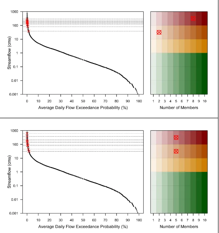
Figure 7 conveys the daily flooding danger at the basin scale by comparing the daily mean HEC-HMS streamflow for each of the 10-members to the basin’s flow-duration curve. The daily mean streamflow for each of the 10-members (represented as a red “X” in the left plots) is shown for April 3, 2017 and June 2, 2016. The right plots of Figure 7 show the simulated daily mean streamflow in a decision support heatmap. The heatmap is designed to convey flooding danger, both in terms of event magnitude and uncertainty of that magnitude through model member agreement.
35
Figure 7. Streamflow risk report for the 2017 (top panel) and 2016 (bottom panel) events. The left panel of each report shows the flow duration curve (black points) generated from the historical daily mean streamflow for USGS 08101000. The simulated daily mean streamflows, taken from averaging the hourly output from HEC-HMS to a daily value, for each ensemble member is represented by a red cross for 04/03/2017 (top panel) and 06/02/2016 (bottom panel). The right panel shows a heatmap of streamflow magnitude and model member agreement. The vertical component of the heatmap represents increasing risk through increasing streamflow magnitude. The horizontal component represents decreasing risk uncertainty through increasing agreement of ensemble members.
36 Both events show at least half of the ensemble members agreeing on a daily mean flow exceeding 100 m3s-1 (Figure 7). The logarithmic scale applied as the Green/Amber/Red decision threshold is arbitrary, but conveniently depicts model agreement by daily streamflow order of magnitude. Figure 7 is intended to be used as preliminary warning because it is comparing to the flow-duration curve which is specific to a single point in the basin and doesn’t necessarily apply to the river crossing infrastructure. Additionally, the flow-duration curve considers daily averages, which masks the peak values associated with a hydrologic response that can occur on the order of hours.
4.3.2 Return Period Analysis
LN(μ, σ) = 1 xσ√2πe −(ln x−μ)2 2σ2 Where: μ = 5.88 σ = 0.94
H0: ln(Streamflow) follows a lognormal distribution HA: ln(Streamflow) does not follow that distribution
Normality Test P-Value
Shapiro-Wilk 0.958
Lilliefors 0.954
Figure 8. The histogram (top left panel, light blue bins) of annual peak streamflow for USGS 08101000 Cowhouse Creek at Pidcoke, Texas spanning the years 1951-2016. A logrithimic distribution (dark blue line) is fit to the peak streamflow. The equation of the log-normally distributed probablity density function (Johnson, Kotz, & Balakrishnan, 1994) and the population parameters for this study are in the top right panel. The units of population parameters are ln[m3s-1]. Hypothesis test p-values for the statistical tests of
distribution normality are in the bottom panel.
The return periods presented are taken from the logarithmic distribution fit to the population of peak flows for the USGS gauge on Cowhouse Creek (Figure 8, blue line). The
37 logarithmic distribution has a mean of 358 m3s-1 and standard deviation of 2.55 m3s-1. The null hypothesis for the testing of statistical significance is the fitted distribution follows a log-normal distribution. The p-values from the Shapiro-Wilk and Lilliefors normality tests are 0.958 and 0.954 respectively. With all p-values greater than an assumed alpha value of 0.05, the decision is to fail to reject the null hypothesis. The statistical tests show that there isn’t significant evidence that ln(streamflow) doesn’t follow a log-normal distribution.
Table 2 shows the return periods, with both observations and model output, for the two hindcasted events. The return periods from observations are 1.6 years (2017) and 6.1 years (2016). The ensemble median return period is the same as observations for the 2017 event, but all ensemble return periods are less than the observed value for 2016. Note the 2016 observation used for the return period calculation (6.1 years) occurs right before the gauge goes offline (see June 3, 2016 04:00 UTC in Figure 5). The return periods in Table 2 show agreement that the two events hindcasted here are not infrequent hydrologic events for this basin.
Table 2. Return periods (in years) compared between observations and simulations. Event peak streamflows are taken from USGS observations and from each of the 10 HEC-HMS simulations. Exceedance probabilities are from the logrithimic distribution seen in Figure 8.
Event Observed Simulated 1st Quartile Simulated Median Simulated 3rd Quartile 2017 1.6 1.4 1.6 2.3 2016 6.1 2.9 4.4 5.4 4.3.3 Detailed Warning
Figure 9 presents a more detailed analysis of the flooding safety risk by looking at a finer hourly temporal resolution and focusing on individual LWXs at Cowhouse Creek. When the preliminary report (Figure 7) flags a potentially dangerous increase in daily mean streamflow, Figure 9 can be used as additional, more detailed, decision support.
38 Figure 9 specifically shows the safety thresholds for LWX #15 on Cowhouse Creek. The uncertainty of the safety risk is conveyed through model agreement and depicted by the intensity of the red/green color. The report shows 100% model agreement of flow characteristics exceeding safety thresholds at LWX #15 on 06/02/2016 16:30 UTC (the time of the accident that claimed nine lives on Owl Creek). Although it is not known what hour the accident occurred in 2017, the report shows 100% model agreement of unsafe conditions for the entire duration of 04/03/2017 (April 3, 2016 05:00 UTC converts to April 3, 2016 00:00 CDT). Additionally, the report shows an exceedance of the safety threshold (at varying levels of model agreement) for the hours (2017) and days (2016) leading up to the two accidents.
39
Figure 9. Hydraulic risk report for the 2017 (top pane) and 2016 (bottom pane) events for LWX 15. The safety threshold is flow velocity mulitplied by flow depth and literature suggests a general value of 0.4 m2/s
as a GO/NO GO for most vehciles. The timeseries of safety threshold is shown for each member by using the streamflow output from HEC-HMS with the rating curves from HEC-RAS. The intensity of the background green/red shows model agreement with darker colors being more memebers above/below the 0.4 m2/s safety threshold. The safety threshold corresponding to the USGS observations is in blue.
40
CHAPTER 5: DISCUSSION
5.1 Precipitation
5.1.1 Intensity and Frequency
The two events hindcasted in this study are fundamentally different in terms of precipitation duration and intensity, but both events claimed lives. The 2017 event was a shorter duration event (precipitation fell for 9 hours on average) of higher intensity, while the 2016 event consisted of less intense rainfall spread out over the period of a week preceding the accident (Fig 4). The differences in storm frequency and duration, but similarity in hydrologic danger, require methods that convey hydrologic risk to be equally cautious of both types of storms.
These events also demonstrate that a large precipitation accumulation, relative to the design storms for this region, is not always necessary to induce a dangerous hydrologic response in the Cowhouse Creek catchment. Precipitation rate return period is not a useful metric for assessing the hydrologic risk for this specific basin. The results highlight that precipitation intensity alone does not correlate to hydrologic response, which supports that other processes, such as those tied to the land surface, could have a strong influence on the magnitude of runoff generation in this basin.
5.1.2 Antecedent Soil Moisture
Both the hindcasted hydrologic events are preceded by precipitation separate from the actual precipitation event corresponding to the deadly flooding. The preceding precipitation events increase the flooding risk of following events by decrease the soil’s availability to store moisture. The preceding events increase soil water content and decrease available void space. Once additional precipitation infiltration increases the soil water content to saturation level, precipitation will stop infiltrating and runoff.
41 The basin soils are primed from the preceding precipitation events in these hindcasts. Additionally, the NLDAS soil moisture observations show that the soils weren’t dry before the preceding precipitation events. The average residual water content of the soils in the Cowhouse Creek basin is 0.09 m3/m3 and the average saturated value is 0.42 m3/m3. The HEC-HMS model is initialized with an average water content of in 0.16 m3/m3 (2017) and 0.27 m3/m3 (2016). The antecedent soil moisture conditions lessen the soil’s available storage. Consequently, more of the precipitation that fell during the hindcasts becomes runoff compared to if the soils were dry. These hindcasts highlight how the land surface state can have a strong influence on the basin’s hydrologic response. If the soils in this basin are presoaked, then consecutive precipitation events characterized by small return periods will trigger a dangerous hydrologic response.
5.2 Hydrology and Hydraulics
5.2.1 Basin Characteristics Shaping Hydrologic Response
Historical data shows that the Cowhouse Creek basin exhibits “flashy” behavior. “Flashy” behavior is a description for steep rising and falling limbs of the hydrograph, as well as short lags times. The characteristics of the basin influence this “flashy” behavior. The landscape is predominately open rangeland and undeveloped (74% grassland/shrub/pasture, 18% forest, and 5% developed by NLCD classification). The lack of impervious surfaces further accentuates the importance of the land surface state being dry or saturated. Also, there isn’t infrastructure on the creek, such as reservoirs to attenuate the streamflow.
The two hindcasted events have short return periods because the histogram in Figure 8 shows that most annual peak flows exceed 190 m3s-1 (the discharge at which the roadbed at Jackson
42 Crossing overtops; distribution mean is 358 m3s-1), meaning that events like the hindcasted ones have occurred nearly annually in the historical record.
The “flashy” behavior is seen when combining the extreme event “pulses” with the shape of the flow-duration curve for Cowhouse Creek. As seen in Figure 7, the 5% exceedance probability corresponds to a daily mean flow less than 10 m3s-1. In other words, the average daily flow is below 10 m3s-1 for 95% of the historical record. The daily flow is dominated by a baseflow signal that doesn’t exceed 1.5 m3s-1 (see Figure 12). The extreme events happen rapidly, on the order of hours, and only a few times a year. The peak flow distribution is characterizing the extreme events, but those same events are being hidden in the flow-duration curve by the dominant signal of the low flows (<10 m3s-1) that characterize this basin for 95% of the year.
5.2.2 Utility of a Probabilistic Framework
Figure 7 shows that there can be large variability in streamflow across the different members, even though they are all generated from the same WRF and HEC-HMS model. The variability of simulated streamflow is attributed to the spatial and temporal precipitation variability across NCAR EPS ensemble members, and this variability “trickling down” through the hydrologic model. The variability of Figure 7 highlights the benefit of using probabilistic methods, such as ensembles, over deterministic methods for forcing predictive hydrologic models. It is important to highlight that the spatial domain of the Cowhouse Creek watershed (1,618 km2) is minuscule compared to that of the weather model ensemble, which is CONUS (~8,000,000 km2). The NCAR ensemble provides data at a 3 km resolution, consequently, the Cowhouse Creek hydrologic model is only forced by 480 grid cells from the ensemble. Therefore, what would be considered small deviations from reality in a weather model at the continental scale could be the difference between the model simulating precipitation within the basin or not, and the consequent