The Potsdam Parallel Ice Sheet Model (PISM-PIK) – Part 1: Model description

www.the-cryosphere.net/5/715/2011/ doi:10.5194/tc-5-715-2011

© Author(s) 2011. CC Attribution 3.0 License.

The Cryosphere

The Potsdam Parallel Ice Sheet Model (PISM-PIK) – Part 1:

Model description

R. Winkelmann1,2, M. A. Martin1,2, M. Haseloff1,3, T. Albrecht1,2, E. Bueler4,5, C. Khroulev5, and A. Levermann1,2

1_{Earth System Analysis, Potsdam Institute for Climate Impact Research, Potsdam, Germany} 2_{Institute of Physics, Potsdam University, Potsdam, Germany}

3_{Department of Physics, Humboldt-University, Berlin, Germany}

4_{Department of Mathematics and Statistics, University of Alaska, Fairbanks, USA} 5_{Geophysical Institute, University of Alaska, Fairbanks, USA}

Received: 15 July 2010 – Published in The Cryosphere Discuss.: 18 August 2010 Revised: 28 July 2011 – Accepted: 22 August 2011 – Published: 14 September 2011

Abstract. We present the Potsdam Parallel Ice Sheet Model

(PISM-PIK), developed at the Potsdam Institute for Climate Impact Research to be used for simulations of large-scale ice sheet-shelf systems. It is derived from the Parallel Ice Sheet Model (Bueler and Brown, 2009). Velocities are calculated by superposition of two shallow stress balance approxima-tions within the entire ice covered region: the shallow ice ap-proximation (SIA) is dominant in grounded regions and ac-counts for shear deformation parallel to the geoid. The plug-flow type shallow shelf approximation (SSA) dominates the velocity field in ice shelf regions and serves as a basal slid-ing velocity in grounded regions. Ice streams can be identi-fied diagnostically as regions with a significant contribution of membrane stresses to the local momentum balance. All lateral boundaries in PISM-PIK are free to evolve, includ-ing the groundinclud-ing line and ice fronts. Ice shelf margins in particular are modeled using Neumann boundary conditions for the SSA equations, reflecting a hydrostatic stress imbal-ance along the vertical calving face. The ice front position is modeled using a subgrid-scale representation of calving front motion (Albrecht et al., 2011) and a physically-motivated calving law based on horizontal spreading rates. The model is tested in experiments from the Marine Ice Sheet Model Intercomparison Project (MISMIP). A dynamic equilibrium simulation of Antarctica under present-day conditions is pre-sented in Martin et al. (2011).

Correspondence to: A. Levermann (anders.levermann@pik-potsdam.de)

1 Introduction

In order to understand the evolution of ice sheets, especially with respect to their contribution to sea-level rise, there is a need for numerical models which are able to capture the dynamics of sheet-shelf systems as a whole. To this end, there are various types of approaches:

Flowline models are both computationally efficient and at the same time very useful for understanding basic processes (e.g., Dupont and Alley, 2005). However, one of the key issues regarding global sea-level rise is the buttressing ef-fect of ice shelves on the sheet which influences the ice flux across the grounding line. In flowline models, this can only be investigated by prescribing a parameterized buttressing strength. Three-dimensional models, by contrast, compute the effect of buttressing for any embayment.

Three-dimensional models which solve the complete Stokes stress balance (e.g., Mart´ın et al., 2004; Jarosch and Gudmundsson, 2007; Pattyn, 2008) cannot be used for large-scale, long-term, high resolution modeling because they are computationally too demanding. The same constraint gen-erally applies to intermediate, so-called higher order models (e.g., Blatter, 1995; Pattyn, 2003).

Models based on the Shallow Ice Approximation (SIA, Hutter, 1983) and the Shallow Shelf Approximation (SSA, Morland, 1987; Weis et al., 1999), each recalled in Sect. 2, decrease these computational costs. They make use of a scal-ing analysis of the full Stokes problem, usscal-ing the fact that ice thickness is small compared to relevant horizontal scales, to enable simulations of whole ice sheets.

SIA-only models (e.g., Greve, 1997; Payne, 1999; Mar-shall et al., 2000) provide a good approximation for the

flow of ice that is frozen to the bedrock. In order to sim-ulate regions of higher velocity such as ice streams, sliding of grounded ice is incorporated in various SIA models by adding a sliding velocity at the base of the ice column which depends directly on the gravitational driving stress.

The SSA has been used to simulate the flow in ice shelves which have no basal friction and thus a different stress regime (e.g., MacAyeal et al., 1996).

The two shallow approximations have been combined us-ing different approaches: some hybrid models (e.g., Huy-brechts, 1990; Ritz et al., 2001) solve the SIA and the SSA in distinct map-plane regions, which results in an abrupt change in flow type across the grounding line. Pollard and Deconto (2009) combine both shallow approxi-mations via a heuristic shear stress correction and an addi-tional grounding line velocity correction based on the one-dimensional approach by Schoof (2007b).

Here, we present the Potsdam Parallel Ice Sheet Model (PISM-PIK), developed at the Potsdam Institute for Climate Impact Research (PIK), a new hybrid model for marine ice sheets. It combines the two approximations by adding the SIA and the SSA velocity on the whole sheet and shelf sys-tem in order to incorporate the different flow regimes in sheet, streams and shelves in a universal manner.

PISM-PIK is based on the Parallel Ice Sheet Model (PISM; Bueler and Brown, 2009), which is a three-dimensional thermodynamically-coupled shallow model us-ing a finite-difference discretization. These models are in-novative in using the SSA as a sliding law for grounded ice, thereby avoiding discontinuities at the onset of sliding, and provide a framework for consistently modeling sheet-shelf systems. Stream-like flow is modeled by the SSA stress bal-ance and a plastic till model for basal mechanics (Schoof, 2006a). In aiming at modeling the Antarctic ice sheet and shelves (Martin et al., 2011), PIK modifications to PISM have been made particularly with respect to the shelf dynam-ics. Ice shelves are especially important for an assessment of past and future sea level contributions of Antarctica be-cause of their buttressing effect on the dynamics upstream of the grounding line and its position (De Angelis and Skvarca, 2003; Bamber et al., 2007; Rott et al., 2007; Glasser and Scambos, 2008; Rignot et al., 2008; Goldberg et al., 2009).

In Sect. 2 we describe PISM-PIK with special focus on the modifications compared to PISM. Section 3 shows its per-formance in experiments from the Marine Ice Sheet Model Intercomparison Project (MISMIP). A summary is given in Sect. 4. The performance of PISM-PIK under present-day boundary conditions for Antarctica is discussed in Martin et al. (2011).

2 Model description

Our description of the model proceeds from the underlying continuum model to the numerical schemes. The major

char-acteristics of the continuum model are adopted from PISM (Sect. 2.1), but modifications include changes to the way slid-ing occurs (Sect. 2.2) and major changes in the treatment of marginal boundaries of the ice sheet and shelves, in particu-lar calving fronts (Sects. 2.4–2.6).

Boundary data provided to PISM-PIK are bed elevationb, surface mass balanceM, geothermal fluxGand ocean tem-peratureTo. In simulations for Antarctica such as the dy-namic equilibrium simulation in Martin et al. (2011), the sur-face temperature distribution is a parameterized function of latitude and elevation, and the model is initialized with ob-served ice thickness data from Lythe et al. (2001) and Le Brocq et al. (2010). In each time step, the model is solved for velocityv, basal melt rateSand calving rateC. Each time step updates the prognostic variables, which are ice tempera-tureT and thicknessH. Because the bed elevationbis fixed in time, each update to the ice thickness implies an update to surface elevationh. (For the notation throughout this paper see Table A1.)

Each of the model equations is numerically discretized, us-ing a finite difference approach on a rectangular grid. Exactly as described in Bueler and Brown (2009), the new model PISM-PIK runs in parallel using the Portable, Extensible Toolkit for Scientific computation (PETSc) for solving every discretized model equation, including the SSA. Time step-ping is explicit and adaptive. Technically speaking, PISM-PIK is implemented as derived classes of the C++code of the open-source Parallel Ice Sheet Model (PISM), version stable0.2 (The PISM authors, 2011).

2.1 Field equations and shallow approximations

For completeness we give a short review of the field equa-tions used both in PISM and PISM-PIK. For more details see Bueler and Brown (2009) and Bueler et al. (2007).

The equation of mass continuity describing the evolution of the ice thickness

∂tH=M−S−∇·Q (1)

can be derived from incompressibility∂µvµ=0 and the

kine-matic equations at the surface and base of the ice. (Through-out this paper, the Einstein summation convention is used.) HereQis the vertical integral of the horizontal velocity. The mass continuity equation is solved numerically forH. The vertical velocityvzwithin the ice

vz(z)= −S+vb·∇b− z

Z

b

∇·vdζ (2)

is also given by incompressibility.

The following shallow equation of conservation of en-ergy includes advection and vertical conduction of heat and a strain dissipation heating term (Greve and Blatter, 2009, Eq. 5.105)

ρici ∂tT+vµ∂µT

=ki∂zz2T+6 . (3)

The strain heating (6) is a function of the second invariant of the strain rate tensor, which is – modifying the approach by Bueler and Brown (2009) – approximated by an unweighted sum of the strain rate tensors of SIA and SSA. Details about the combination of SIA and SSA in PISM-PIK compared to PISM are given in Sect. 2.2.

Surface temperature Ts and the geothermal flux as well as pressure melting temperature in the case of ice shelves provide boundary conditions for this equation.

Equation (3) is solved for the temperature on a z-coordinate system, where the z-z-coordinate measures the ver-tical distance above the bedrock for grounded ice and above the ice shelf base for floating ice, so the zero level for z is always the base of the ice. This grid choice, and thermome-chanical verification results from PISM using it, are docu-mented in (Bueler et al., 2007).

The flow law is given by

˙ ij≡

1 2

∂vi ∂xj

+∂vj ∂xi

=EA(T∗)q(1/2)τijτij

n−1 τij (4)

withn=3. Here,˙ is the strain rate tensor andτ the devia-toric stress tensor withτij=σij+pδij where the pressurepis

the isotropic part of the full stress tensorσ. Throughout this paper, the tensor indicesi andj denote the two horizontal components of vertically-integrated terms.

Following Paterson and Budd (1982), ice softnessA(T∗) is given by

A(T∗)= (

(3.61×10−13)e−6.0×104/(RT¯ ∗), T∗≤263.15 K,

(1.73×10+3)e−13.9×104/(RT¯ ∗), T∗>263.15 K. (5) The flow law has an inverted form

τij=2ν˙ij (6)

in which the effective viscosityν depends on the effective strain rate and the temperature.

The Stokes stress balance for a viscous fluid (Greve and Blatter, 2009, Sect. 5.1) is approximated using two limiting shallow approximations.

The Shallow Ice Approximation (SIA, Morland and John-son, 1980; Hutter, 1983) is valid for regions where bot-tom friction is high enough for the vertical shear stresses to dominate over the horizontal shear stresses and longitudinal stresses. The corresponding velocities are given by

vSIA=−2(ρig)n|∇h|n−1 

 z Z

b

ESIAA(T∗)(h−ζ )ndζ 

∇h. (7)

The second shallow approximation is the Shallow Shelf Approximation (SSA, Morland, 1987; Weis et al., 1999) for which the stress balance reads

∂ ∂x

2νH¯

2∂vx

∂x + ∂vy

∂y

+ ∂ ∂y

¯ νH

_∂v

x ∂y +

∂vy ∂x

+

τbx=ρigH

∂h

∂x (8)

∂ ∂x

¯ νH

_∂v

x ∂y +

∂vy ∂x

+ ∂

∂y

2νH¯ _∂v

x ∂x +2

∂vy ∂y

+

τby=ρigH

∂h

∂y. (9)

Here,τb=(τbx,τby)denotes the basal shear stress.

The vertically-averaged effective viscosity is given by

¯ ν=

¯ B

2(ESSA)

−1 n

₁ 2˙ij˙ij+

1 2˙

2 ii

1₂−_nn

(10)

whereB¯is the vertically-averaged ice hardness,˙is the strain rate tensor andESSAis an enhancement factor.

The SSA stress balance is non-local, i.e., when solving for the velocity at a certain grid point, the solution will depend on the whole spatially-distributed stress field.

In an ice shelf where there is zero traction at the base of the ice, the driving stress is exclusively balanced by membrane stresses (those stresses held by viscous deformation), and the basal shear stress is set to zero (τb=0). The resulting plug flow is described by the SSA, see the upper panel in Fig. 1 (ice shelf ).

Following MacAyeal (1989), the Shallow Shelf Approx-imation is also used for modeling the fast flow regime in ice streams (see the upper panel in Fig. 1; ice stream). Ice streams have a flow-regime similar to the one in ice shelves (a plug flow) but experience basal resistance. Thus, Eqs. (8) and (9) are used with nonzero basal frictionτb, which is cal-culated based on a model for plastic till (Schoof, 2006a) τbi= −τc

vi

v2

x+vy2

1/2. (11)

This basal model assumes that till supports applied stresses without deformation until these equal a yield stressτc. Di-vision by zero is avoided by the addition of a small constant in the denominator (Bueler and Brown, 2009). Yield stress is given by the Mohr-Coulomb model for saturated till, with till cohesionc0set to zero (Paterson, 1994)

τc=c0+(tanφ)(ρigH−pw) . (12)

The porewater pressure is parameterized by

pw=0.96ρigH λ. (13)

whereλranges from 0 to 1 and can be interpreted as water content in the till. A specific parameterization ofλ depend-ing on bed elevation and sea level is given for Antarctica in Martin et al. (2011).

1300 1400 1500 1600 1700 1800 1900 2000 2100 2200 2300 −500

0 500 1000 1500

distance from (83.4 S, 0 E)(km)

v

e

lo

c

it

y

(

m

/a

)

−1500 −1000 −500 0 500 1000 1500 2000 2500 3000

ic

e

p

ro

fi

le

° °

ice sheet ice stream ice shelf

SIA v

SIA v

b v = vb SSA v SIA 0

SSA v

∼∼

∼

∼

Fig. 1: Superposition of SIA and SSA velocities.

Upper panel: Schematic diagram of ice profile and different flow regimes. Throughout the grounded

ice region, the ice velocity is determined by linear superposition of the SIA (blue arrows) and the

SSA velocities (red arrows).

Ice sheet

with negligible basal sliding. The velocity is dominated by

the Shallow Ice Approximation. Friction at the bed leads to shearing in the ice column and a velocity

profile as depicted in blue.

Ice stream. Both SIA and SSA velocities are relevant for the ice flow.

The SSA serves as a sliding law for the shear flow.

Ice shelf. The plug flow regime is dominated by

the SSA leading to a uniform vertical velocity profile.

Lower panel: An example cut through the sheet-stream-shelf transition of the Lambert Glacier and

Amery Ice Shelf in the equilibrium simulation described in Martin et al. (2011). The model output

velocity

v

=

v

+

v

is shown in black. The onset of an ice stream is diagnosed to be where the

SSA velocity (red) exceeds the SIA velocity (blue).

21

Fig. 1. Superposition of SIA and SSA velocities. Upper panel: schematic diagram of ice profile and different flow regimes. Throughout the grounded ice region, the ice velocity is determined by linear superposition of the SIA (blue arrows) and the SSA velocities (red arrows). Ice sheet with negligible basal sliding. The velocity is dominated by the Shallow Ice Approximation. Friction at the bed leads to shearing in the ice column and a velocity profile as depicted in blue. Ice stream. Both SIA and SSA velocities are relevant for the ice flow. The SSA serves as a sliding law for the shear flow. Ice shelf. The plug flow regime is dominated by the SSA leading to a uniform vertical velocity profile. Lower panel: an example cut through the sheet-stream-shelf transition of Lambert Glacier and Amery Ice Shelf in the equilibrium simulation described in Martin et al. (2011). The model output velocityv=vSIA+vSSAis shown in black. The onset of an ice stream is diagnosed to be where the SSA velocity (red) exceeds the SIA velocity (blue).

2.2 Velocity combination, sliding and grounding line motion

Following the basic idea of superposition of SIA and SSA from Bueler and Brown (2009), both SIA and SSA velocities are computed on the whole model domain in PISM-PIK, en-abling a smooth transition both from non-sliding ice which is frozen to the bedrock to faster-flowing ice in regions where significant sliding occurs, and from rapidly-sliding ice across the grounding line to floating ice (indicated in Fig. 1).

Bueler and Brown (2009, Eqs. 21 and 22) use a weighting function in order to combine the SIA and SSA velocities in the PISM base version

v=f (|vSSA|)vSIA+(1−f (|vSSA|))vSSA (14) where |vSSA| =v2_SSAx+v2_SSAy. The weighting function f (|vSSA|)ensures a continuous solution of the velocity from

the interior of the ice sheet across the grounding line to the ice shelves. It is approximately 1 for small|vSSA| and ap-proximately 0 for large|vSSA|so that the SIA velocity fully governs the overall velocity where the SSA velocity is small (in the interior of the ice sheet). However, the choice of the weighting function is an additional degree of freedom which is not constrained by observations and is therefore not used in PISM-PIK. Instead, the contributions resulting from the two approximations are simply added, still ensuring a smooth transition of the velocity across the grounding line. Thus in PISM-PIK the basal velocities for grounded ice are the SSA velocitiesvb=vSSAand

v=vSIA+vSSA. (15)

On ice shelves, experiments with simplified setups have shown that the SIA contribution is negligible due to the low

surface gradient so that the dynamics there are dominated by the SSA. In the inner part of the sheet where bottom friction is high enough for vertical shear to dominate over horizon-tal shear, the SSA contribution is negligible so that the ice velocity there is dominated by the SIA contribution.

This SIA/SSA hybrid scheme provides an alternative to SIA-only thermomechanically-coupled sliding models, which allow sliding using evolving basal resistance fields and are generally subject to the failures described quali-tatively and quantiquali-tatively in Appendix B of Bueler and Brown (2009). In these cases, where sliding is incorporated by adding a basal velocity vb to the SIA velocity vSIA in Eq. (7), unbounded vertical velocities arise from (physically-possible) abrupt changes in basal strength (Fowler, 2001; Bueler and Brown, 2009). The ISMIP-HEINO experiments (Calov et al., 2010), in particular, demonstrate the diffi-culty such models generally experience with dynamically-evolving basal resistance fields. Through the superposition of the two velocity fields, each of which are differentiable, unbounded vertical velocities cannot arise with the hybrid scheme used in PISM-PIK.

The basic, mathematical task of model verification is car-ried out in Bueler and Brown (2009) and Bueler et al. (2007) and references therein. But especially the question whether the dual approximation used here is indeed a valid approxi-mation of the Stokes equations in the transition zone needs to be deferred to other publications. A comparison of the super-position approach to Blatter-Pattyn type models or other “hy-brid solvers” like in Pollard and Deconto (2009), Schoof and Hindmarsh (2010), and Goldberg (2011) and performance in ISMIP-HOM would be most interesting as well but is beyond the scope of this paper.

The SIA/SSA hybrid scheme enables the model to simu-late qualitatively different flow regimes – fast as well as slow processes. Martin et al. (2011) show that the velocities in an equilibrium simulation of Antarctica span several orders of magnitude, from almost zero close to the ice divides over ve-locities of a few meters per year in large areas of the interior of the ice sheet to the highest velocities of sliding grounded ice which are associated with stream-like features and reach a few kilometers per year.

We diagnose an ice stream as a region where the SSA ve-locities are larger than the contribution from the SIA veloci-ties to the vertically averaged overall velocityv, i.e.,¯

vb>v¯−vb. (16)

This definition is purely diagnostic and no different physics are prescribed. It serves as a simple way of identifying the parts of the sheet with significant sliding.

The lower panel in Fig. 1 from the dynamic equilibrium simulation discussed in Martin et al. (2011) illustrates how the modeled velocity undergoes a qualitative change from non-sliding over sliding to floating ice. Here, the velocity contributions from SIA (in blue) and SSA (in red) are shown

for an example cut through the modeled Lambert Glacier and Amery Ice Shelf. An ice stream is identified as the grounded region where the SSA velocity supersedes the SIA velocity and is understood as the transition region between the sheet without significant sliding where the velocity is almost en-tirely given by the SIA velocity and the floating shelf where the SSA velocity clearly dominates.

The second merit of the hybrid scheme is the stress trans-mission across the grounding line. In PISM-PIK, the ground-ing line is not subject to any boundary conditions. Its posi-tion is determined in each time step via a mask which dis-tinguishes grounded ice from floating ice using the flotation criterion

b(x,y)= −ρi ρo

H (x,y). (17)

The grounding line motion is thus influenced indirectly by the velocities through the ice thickness evolution. Since the SSA velocities are computed non-locally and simultaneously for the shelf and for the sheet, a continuous solution over the grounding line without singularities is ensured and buttress-ing effects are accounted for.

In Sect. 3, the reversibility of the grounding line migra-tion on a sloping bed with PISM-PIK is demonstrated in ex-periments from the Marine Ice Sheet Model Intercompari-son Project (MISMIP). The variability of the grounding line under climate forcing is additionally demonstrated in an ex-periment shown in the supplement of Martin et al. (2011) where a sinusoidal surface temperature forcing is applied to an equilibrium state of Antarctica, resulting in forward and backward motion of the grounding line.

2.3 Discretization scheme for mass transport

PISM uses a mass continuity scheme for SIA fluxes which has perfect numerical mass conservation (Bueler et al., 2005). The low-order mass continuity scheme used for SSA fluxes, as described in Bueler and Brown (2009), however, can lead to local mass conservation errors. Keeping track of all mass fluxes and comparing their sum to the change in total ice volume has shown that especially at ice margins problems arise.

We employ a modified scheme in PISM-PIK that is lo-cally mass conserving and that applies to both SIA and SSA velocities in the same way. As in PISM, in general the SSA velocities are computed on the regular grid whereas the SIA velocities are computed on a staggered grid, i.e., on a grid which is shifted by half a grid length compared to the regu-lar grid. For the discretization of the mass transport, the SSA velocities are transferred onto that same staggered grid by av-eraging over the SSA velocities from the adjacent grid cells. The sum of the SIA and SSA velocities on the staggered grid is the total velocity which is used in a mass-conserving up-wind finite difference scheme for the mass continuity Eq. (1):

1Hi

1t = (18)

− 1 1x     

vi+ 1 2

x Hi, v i+1

2 x >0 vi+

1 2

x Hi+1, v i+1

2 x ≤0

−   

vi− 1 2

x Hi−1, v i−1

2 x >0 vi−

1 2

x Hi, v i−1

2 x ≤0

.  

An analogous equation holds for the y-component. This scheme ensures mass conservation since every contribution of mass inflow in one box is necessarily a contribution to mass outflow in an adjacent box.

At the ice front the scheme needs to be slightly modified, since we do not compute velocities in ocean-boxes without ice. To avoid the zero velocity contribution of the ocean box adjacent to the last shelf box, when computing the staggered velocity at the calving front, we use the unstaggered SSA velocity from this last shelf box and the front stress boundary condition.

The properties of this alternative scheme for the pure-SIA mass continuity problem have been tested by comparison to the similarity solution described by Halfar (1983), and the deviations of this solution when using the PISM-PIK scheme are of the same order of magnitude as the ones when using the PISM base version (Bueler et al., 2005). For the SSA, Albrecht et al. (2011) have shown that the analytical solution for the flow line case from Van der Veen (1983) for an ice shelf in equilibrium is better approximated with this alterna-tive mass transport scheme than with the scheme described in Bueler and Brown (2009). It is not necessary to modify the adaptive time-stepping from PISM base version to ensure the numerical stability of this scheme.

2.4 Calving front stress boundary condition

At the calving front, the imbalance between vertically-integrated stresses in the ice and the hydrostatic pressure ex-erted by the ocean contributes to the ice flow upstream of the calving front. A calving front stress boundary condi-tion is necessary for solving the non-local SSA momentum balance Eqs. (8) and (9). PISM-PIK therefore incorporates a physical stress boundary condition (Weertman, 1957; Mor-land and Zainuddin, 1987) describing the stress imbalance at the calving front. By contrast, in PISM there is no such condition, and instead a notional ice shelf extends across the ice-free ocean to the edge of the computational domain. The choice of the ice thickness and viscosity used for such an extension and the effect on the rest of the modeled ice are inadequately understood (MacAyeal et al., 1996; Bueler and Brown, 2009). The stress boundary condition implemented in PISM-PIK reads

zsl+

1−ρi

ρo

Hc Z

zsl−ρρoiHc

σµν·nνdz=

1 2ρog

_ρ i ρo

Hc 2

ni, (19)

wherezsl denotes the sea-level, Hc is the ice thickness at the calving front and n=(nx,ny) the horizontal,

seaward-pointing vector normal to the calving front.

The SSA stress balance Eqs. (8) and (9) can be expressed in terms of a vertically-integrated stress tensor (Schoof, 2006b)

Tij≡2νH¯ ˙ij+ ˙kkδij

. (20)

This gives the SSA stress balance a very compact form which is equivalent to Eqs. (8) and (9) combined:

∂Tij

∂xj

+τbi=ρigH

∂h

∂xi

. (21)

The deviatoric part of the left hand side of the stress boundary condition can then be expressed in terms of the vertically integrated deviatoric stress tensor

Tij≈

Z

dzτij=

Z

dz 2ν˙ij. (22)

Neglecting air pressure and assuming cryostatic pressure in the ice we get

Tijnj=

1 2

1−ρi

ρo

ρigHc2ni. (23)

In terms of SSA velocities vx,vy

, ¯

νHc

2∂vx ∂x+

∂vy ∂y

nx+

1 2 _∂v x ∂y + ∂vy ∂x ny

=τstatnx,(24)

¯ νHc

_∂v

x ∂x+2

∂vy ∂y

ny+

1 2 _∂v x ∂y + ∂vy ∂x nx

=τstatny.(25)

The right-hand side of these equations, representing the static part of the stress balanceτstat, is computed according to the type of ice front concerned. In PISM-PIK, we distinguish be-tween three types of ice-ocean interfaces, namely shelf calv-ing fronts where

τstat=τstatsf ≡ ρigHc2

4

1−ρi ρo

, (26)

marine ice fronts (ice at the coast resting on bedrock below sea level) where

τstat=τstatmf≡ ρig

4

H_c2−ρo ρi

(zsl−b(x,y))2

(27) and cliffs (ice at the coast resting on bedrock above sea level) where

τstat=τstatcl ≡ ρigHc2

4 . (28)

These stress boundary conditions are applied directly at the calving front by replacing certain terms in the discretiza-tion of the SSA equadiscretiza-tions with the respective terms from the boundary condition, making the use of an artificial shelf ex-tension obsolete. The implementation holds for any shape of calving front and is described in detail in Appendix A.

z

ice shelf

ocean

atmosphere

z

x

net force

Fig. 2: Schematic diagram of forces at the calving front. Hydrostatic pressure (gray arrows) and

cryostatic pressure (black arrows) result in net force in direction of the ocean (blue arrow). The net

force is significantly reduced compared to a situation where the hydrostatic pressure is neglected.

22

Fig. 2. Schematic diagram of forces at the calving front. Hydro-static pressure (gray arrows) and cryoHydro-static pressure (black arrows) result in a net force in direction of the ocean (blue arrow). The net force is significantly reduced compared to a situation where the hydrostatic pressure is neglected.

2.5 Continuous ice shelf advance and retreat through subgrid parameterization

In order to capture subgrid-scale advance and retreat of the calving front as depicted in Fig. 3 the mechanism introduced by Albrecht et al. (2011) is implemented in PISM-PIK.

The subgrid parameterization is a precondition for the ap-plication of a continuous calving law like the one described in Sect. 2.6 because it models the observed almost vertical cliff-like shape of the calving fronts and preserves realistic driving stresses and hence spreading rates near the ice edge.

Without this mechanism the ice flux into a newly occupied grid cell would be spread out over the entire horizontal do-main of that cell, possibly resulting in ice shelf grid cells of only a few meters ice thickness or less. The front of these cells would propagate one grid cell ahead in each time step, leading to an unphysical extension of the ice shelf onto the ocean.

In particular, for an advancing ice front, the discretized version of the mass continuity equation yields a volume in-crementV for each cell at the ice front that needs to be added to the adjacent ocean grid cell. Without the subgrid parame-terization, the volume increment would cover the whole area of this adjacent ocean grid cell and the newly formed shelf would be unrealistically thin. In order to avoid this purely numerical effect, in PISM-PIK a fieldRis introduced which gives the ratio of ice-covered horizontal area in each grid-cell depending on a reference ice thicknessHr, equal to the mean ice thickness of the adjacent full shelf grid cells of the previous time step:

R= V aHr

(29) wherea is the area of the grid-cell andR takes values be-tween 0 and 1,R=1 corresponding to full ice-shelf cells and

R=0 to ice-free ocean cells. Thus, for a cell with 0< R <1, the area Ra is covered with ice of the same thickness as the mean of the adjacent full shelf grid cells as illustrated in Fig. 3.

Concerning the mass budget for the partially-filled cells, the outflow is determined by the calving rate while the in-flow is computed from the ice thickness at the front and the velocities on the staggered grid described in Sect. 2.3.

A retreat of the calving front can be modeled in the same manner: first, the calving rate is determined through the calv-ing law described in Sect. 2.6. The amount of mass lost through transport by this calving rate is removed by changing the ice volume in the partially-filled cells at the ice front, and, as needed, by transforming adjacent filled cells into partially-filled cells.

2.6 Calving law

Based on the observation by Doake et al. (1998) and Alley et al. (2008) that the calving rate is linearly-related to the product of near-front thickness, half-width and strain rate, a local first-order law for large-scale ice shelf calving was introduced by Levermann et al. (2011) as a boundary con-dition to the mass continuity equation. This so-called Eigen Calving law has been implemented in PISM-PIK.

The applied calving rate is based on the eigenvalues˙±of

the horizontal strain rate tensor (see Eq. 4). Along most areas of the calving front the corresponding eigen-directions will coincide with the directions parallel to and transverse to the flow (Fig. 4). In regions of divergent flow, where spreading occurs in both principle directions (˙±>0), we define the rate

of large-scale calving as

C=Kdet(˙)=K˙+˙− for ˙±>0 (30)

withK>0 being a proportionality constant. Else, the calving rate is zero.

Typically, the maximum spreading rate in an ice shelf can be found along the ice-flow direction downstream of, but close to, the grounding line. If the calving rate were to de-pend only on ˙+, it would therefore increase towards the

grounding line so that no stable ice-shelf front would de-velop. Stability arises through the dependence on the product of˙+and˙−since calving is prohibited where˙+˙−is

neg-ative.

Spreading rate fields and therefore areas of potential calv-ing accordcalv-ing to Eq. (30) are strongly influenced by the ge-ometry of an shelf ice. In areas where it comes to conver-gence of ice flow the calving rate is zero whereas it strongly increases where ice flow expands, e.g., at the mouth of an embayment, hindering the shelf to grow outside the embay-ment.

Martin et al. (2011) show that this new dynamically mo-tivated calving law enables PISM-PIK to reproduce realistic calving front positions for many of the ice shelves attached to

a

i-2 i-1 i i+1 i+2

b

i-2 i-1 i i+1 i+2

Hr

Fig. 3: (From Albrecht et al., 2011) Schematic diagram illustrating subgrid-scale advance of the

calving front. As a new grid celli+1is partially filled with ice its ice thickness is kept constant at

the same value as grid celli.

23

Fig. 3. (From Albrecht et al., 2011) Schematic diagram illustrating subgrid-scale advance of the calving front. As a new grid celli+1 is partially filled with ice its ice thickness is kept constant at the same value as grid celli.

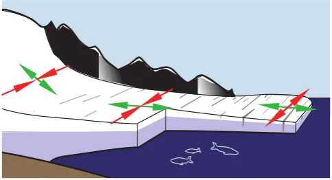
Fig. 4: Schematic diagram of calving law (see Eq. 30). Green arrows denote the eigen-direction

along the flow direction, red arrows the eigen-direction perpendicular to the flow direction.

Con-vergence of ice flow perpendicular to the main flow direction is associated with closure of crevasses

whereas spreading in both directions (corresponding to positive eigen-values±˙ ) is associated with

intersecting crevasses and enhanced calving.

24

Fig. 4. Schematic diagram of calving law (see Eq. 30). Green ar-rows denote the eigen-direction along the flow direction, red arar-rows the eigen-direction perpendicular to the flow direction. Conver-gence of ice flow perpendicular to the main flow direction is as-sociated with closure of crevasses whereas spreading in both direc-tions (corresponding to positive eigen-values˙±) is associated with

intersecting crevasses and enhanced calving.

the Antarctic ice sheet, across a broad range of ice thickness values.

Due to the calving law, an ice bridge connecting the main part of an ice shelf and a wider tongue can be calved off and the thereby separated tongue forms an iceberg of the size of a few grid cells. For these floating pieces with zero to-tal basal resistance the SSA does not have a unique velocity solution (Schoof, 2006b). Therefore they are identified and eliminated, and their volume is reported as lost through calv-ing.

Since no subgrid interpolation is implemented for marine fronts and ice cliffs, mass loss occurs as follows in these cases: in each timestep, a small amount of ice is transported from a grid cell at the marine front or ice cliff into the adja-cent ocean grid cell. The hereby emerging shelf cells contain typically very thin ice and therefore calve off immediately.

3 Experiments from the Marine Ice Sheet Model Intercomparison Project

The numerical performance of PISM-PIK was tested in the context of the Marine Ice Sheet Model Intercomparison Project (MISMIP, Schoof et al., 2009). The results of these simulations allow a comparison with the semi-analytical so-lution by Schoof (2007a), and give insight into the quality of the numerical treatment of grounding line motion. Note that grounding line migration results directly from the flota-tion criterion and is thus fully determined by the dynamics described in Sect. 2.

We consider only the MISMIP flow-line experiments on a constant slope bed (experiments 1 and 2) in this paper. As PISM-PIK is a three-dimensional model, a flow-line was simulated using periodic boundary conditions in the cross-flow direction. Calving occurs at a fixed position in MISMIP so the calving law in Sect. 2.6 was not used. The model was run at resolutions of 12 km, 6 km and 3 km. Upon changes in flow parameterA(Eq. 5), the position of steady-state ground-ing line should closely follow the semi-analytical solution, depicted as a solid black line in Fig. 5a. In order to diagnose the position of the grounding line at subgrid scale, a refine-ment based on Pattyn et al. (2006) was introduced for the analysis of the MISMIP experiments.

During experiment 1 the softness parameterAis lowered stepwise. During experiment 2 these changes are reversed. Figure 5a shows the modeled grounding line position. It can be seen that (i) the movement of the grounding line is mod-eled qualitatively correctly at all resolutions, (ii) an offset from the semi-analytical solution is observed in experiment 1, and (iii) the offset is smaller in experiment 2. The offset in experiment 1 decreases with increasing resolution, while in experiment 2 it is independent of the resolution. The de-pendence on the resolution becomes evident in Fig. 6 which shows the steady-state grounding-line position of experiment 1 for various resolutions. The simulated grounding line po-sitions converge to the semi-analytical solution upon grid-refinement.

0.1 1 10

(a)

A (1e−25 s

−1

Pa

−3

)

Analytical sol. exp. / resol. . 1 / 12 km 1 / 6 km 1 / 3 km 2 / 12 km 2 / 6 km 2 / 3 km

0 500 1000 1500

0 2000 4000

(b)

grounding line position (103 m)

Fig. 5: MISMIP experiments on a constant slope bed.(a)Dependence of grounding-line position

on rate factorA. Solid black line: semi-analytical prediction. Colored lines: simulation results with

PISM-PIK, at∆x=12, 6, 3 km resolution.(b)Example ice sheet profile.

25

Fig. 5. MISMIP experiments on a constant slope bed. (a) Depen-dence of grounding-line position on rate factorA. Solid black line: semi-analytical prediction. Colored lines: simulation results with PISM-PIK, at1x=12, 6, 3 km resolution. (b) Example ice sheet profile.

For a flow-line setup governed by the SSA as consid-ered here, the existence of a shelf should not influence the grounding-line movement in the continuum model (Schoof, 2007a). In the implementation of the problem in PISM-PIK, however, we observe some (numerical) influence of the calving-front treatment on the steady-state results at low res-olutions. This is due to the fact that the SSA stress balance equations are solved simultaneously for the entire computa-tional domain encompassing sheet and shelf.

The implementation of the calving front stress boundary condition (see Sect. 2.4) in PISM-PIK distinctly improves the performance compared to PISM which uses a notional shelf extension in ice-free ocean. This shelf extension method generates a less-accurate backstress on the whole ice body influencing the grounding line position. The subgrid inter-polation of the calving front as described in Sect. 2.5 ensures a controlled shelf growth, while without this treatment a very thin shelf develops immediately. Figure 6 shows that ground-ing line position performance with a subgrid treatment of the calving front is generally better than without, especially at low resolutions.

4 Conclusions

The large-scale marine ice sheet model PISM-PIK presented in this paper is based on the Parallel Ice Sheet Model (PISM), with major modifications for ice shelf dynamics. A boundary condition for the SSA equations capturing the stress imbal-ance at the ice front was incorporated and a novel subgrid

12 6 3 2 1.5 750

800 850 900 950 1000 1050 1100

resolution (km)

grounding line position (10

3 m)

No subgrid Subgrid Analytical sol.

Fig. 6: Grounding-line position vs. resolution for experiment 1, step 1 of MISMIP. Green: with

sub-grid treatment of the calving front motion, blue: without. Black line: semi-analytical prediction.

26

Fig. 6. Grounding-line position vs. resolution for experiment 1, step 1 of MISMIP. Green: with sub-grid treatment of the calving front motion, blue: without. Black line: semi-analytical prediction.

scheme for the advance and retreat of the calving front was introduced. This was combined with a physical calving law which is universal in the sense that it governs the calving process for different shelf geometries.

Grounded ice flow is captured as a direct superposition of velocities from two shallow approximations, SIA and SSA, a modification of the Bueler and Brown (2009) scheme. Both shallow approximations are solved simultaneously in the whole ice area. The new hybrid scheme allows for the treatment of all flow regimes in a consistent manner and per-mits a diagnostic definition of ice streams. PISM-PIK thus includes a treatment of the transition from vertical-shearing dominated flow, in areas where the ice is frozen to the bed, to plug flow in ice shelves. All this governs the ice flux across the grounding line whose position is determined di-rectly from the flotation criterion, so no boundary conditions are imposed to model its motion. Since the SSA velocities are computed non-locally and simultaneously for shelf and sheet, stress transmission across the grounding line is guar-anteed.

The performance of PISM-PIK was tested in context of the Marine Ice Sheet Model Intercomparison Project. In these experiments, the model reproduced the semi-analytically predicted grounding line position dependence on ice softness for the flow-line case, with convergence towards the semi-analytical solution with grid refinement.

As a first application, Martin et al. (2011) present a dy-namic equilibrium simulation for Antarctica, demonstrating the ability of PISM-PIK to simulate whole sheet-shelf sys-tems.

j+1

j

j-1

i

i+1

i-1

b+

b-a+

a-a

a

a

a

b-

b

b

b-

Fig. 7: Stencil for the SSA boundary condition in the case of an ice-filled (white) cell with ice-filled and ice-free (shaded) neighbors. For this specific shape of the calving front the boundary indicators

a−,b+anda−N,a+N,b+W have the value 1, whereasa+,b−anda−S,a+S,b−W,b−E,b+Ehave

value 0.

27

Fig. 7. Stencil for the SSA boundary condition in the case of an ice-filled (white) cell with ice-ice-filled and ice-free (shaded) neighbors. For this specific shape of the calving front the boundary indicators a−,b+anda−N,a+N,b+W have the value 1, whereasa+,b−and a−S,a+S,b−W,b−E,b+Ehave value 0.

Appendix A

On the discretization of the calving front stress boundary condition

In the following we detail the implementation of the calv-ing front boundary condition into the SSA-scheme. We only describe the scheme for SSA Eq. (8). The second equation based on Eq. (9) is similar. Discretizing the outer derivatives of Eq. (8) yields

2

1x(νH )¯ |

j i+1

2

2∂vx

∂x+ ∂vy ∂y j

i+1₂

− 2

1x(νH )¯ |

j i−1

2

2∂vx

∂x+ ∂vy ∂y j

i−1₂

+ 1

1y(νH )¯ |

j+1₂

i _∂v x ∂y + ∂vy ∂x

j+1 2

i

− 1

1y(νH )¯ |

j−1₂

i _∂v x ∂y + ∂vy ∂x

j−1 2

i

=ρigH

∂h

∂x.

The next step is to replace the four expressions of the form

2∂v{ij}

∂{ij}+ ∂v{ij}

∂{ij}

with the respective terms from the boundary condition (24). Using the boundary-indicators a±,b± (see

Fig. 7) leads to

a+

2 1x(¯νH )|

j i+1

2

2∂vx

∂x+ ∂vy ∂y j

i+1₂

−a−

2 1x(¯νH )|

j i−1

2

2∂vx

∂x+ ∂vy ∂y j

i−1₂

+b+

1 1y(νH )|¯

j+1 2 i ∂vx ∂y+ ∂vy ∂x

j+1 2

i

−b−

1 1y(νH )|¯

j−1 2 i ∂vx ∂y+ ∂vy ∂x

j−1 2

i

=ρigH ∂h

∂x+(a+−a−) 2 1xτstat,

wherea±,b±=0 if one or both of the adjacent cells are

ice-free, anda±,b±=1 otherwise, and where the value ofτstat

Table A1. Table of symbols.

Symbol Description SI units

A(T∗) ice softness Pa−3s−1

a area of a grid cell m2

B(T∗) ice hardness;B(T∗)=A(T∗)−n1 _{Pa s}1/3

¯

B vertically averaged ice hardness ¯

B=H−1Rh

bB(T∗)dz

Pa s1/3

b bedrock elevation m

C calving rate m s−1

ci specific heat capacity for ice J (kg K)−1 ESIA enhancement factor for the SIA

ESSA enhancement factor for the SSA

g acceleration due to gravity m s−2 h upper surface elevation of ice m

H ice thickness m

Hc ice thickness at calving front m Hr reference ice thickness m {i,j} 2-D horizontal tensor indices

K proportionality constant for Eigen Calving m s ki thermal conductivity of ice W (K m)−1 M ice equivalent surface mass balance m s−1 n Glen flow law exponent

ni componentiof the seaward pointing normal vector

at calving front

p pressure=isotropic part of full stress tensor: p=1/3σ_kk

Pa=N m−2

pw pore water pressure N m−2

Q horizontal ice flux m2s−1 R ratio of ice-covered horizontal area in

a grid cell ¯

R gas constant J (mol K)−1

S ice equivalent basal mass balance (S>0 is melting)

m s−1

T ice temperature K

T∗ pressure-adjusted temperature K Tij component of the vertically integrated

deviatoric stress tensor

Pa m=N m−1

v overall horizontal ice velocity m s−1

vb basal ice velocity;vb=vSSA=(vx,vy) m s−1 vSIA SIA velocity of ice m s−1

vSSA SSA velocity of ice;vSSA=(vx,vy) m s−1

(x,y) horizontal dimensions m

z vertical dimension (positive upwards) m

zsl sea level m

∂ partial derivative δij Kronecker delta

1x,1y horizontal grid size m

∇ 2-D gradient operator∇=(∂x,∂y) m−1

˙

ij component of the strain rate tensor s−1

˙

± eigenvalues of strain rate tensor s−1 {µ,ν} 3-D tensor indices

ν viscosityν=1/2B(T∗)(1−n)/n Pa s ¯

ν effective viscosity Pa s

ρi density of ice kg m−3

ρo density of ocean water kg m−3 σij full Cauchy stress tensor;σij=τij−pδij Pa=N m−2 τb basal shear stress on ice Pa=N m−2

τc yield stress Pa=N m−2

τij component of the deviatoric stress tensor;

τij=2ν˙ij

Pa=N m−2

τstat vertically integrated static stress at calving front

Pa m=N m−1

φ till friction angle ◦

is determined by one of Eqs. (26), (27) or (28). The calv-ing front is situated at the border between ocean cells and the last completely-filled shelf cells; the stress boundary condi-tion is not applied to partially-filled cells that arise due to the subgrid parameterization described in Sect. 2.5.

Further discretization yields:

a+

4 1x(¯νH )|

j i+1

2 " ∂vx ∂x j

i+1 2

+1 8 b+E

∂vy ∂y

j+1 2

i+1

+b−E

∂vy ∂y

j−1 2

i+1

+b+

∂vy ∂y

j+1 2

i

+b−

∂vy ∂y

j−1 2

i

!#

−a−

4 1x(¯νH )|

j i−1₂

" ∂vx ∂x j

i−1₂

+1 8 b+

∂vy ∂y

j+1₂

i +b− ∂vy ∂y

j−1₂

i

+b+W

∂vy ∂y

j+1₂

i−1

+b−W

∂vy ∂y

j−1₂

i−1 !#

+b+

1 1y(¯νH )|

j+1₂

i " ∂vx ∂y

j+1₂

i

+1 4 a+N

∂vy ∂x

j+1

i+1₂

+a+ ∂vy ∂x j

i+1₂

+a−N

∂vy ∂x

j+1

i−1₂

+a−

∂vy ∂x j

i−1₂

!#

−b−

1 1y(¯νH )|

j−1 2 i " ∂vx ∂y

j−1₂

i

+1 4 a+

∂vy ∂x j

i+1 2

+a+S

∂vy ∂x

j−1

i+1 2 +a− ∂vy ∂x j

i−1 2

+a−S

∂vy ∂x

j−1

i−1 2

!#

=ρigH|ji

∂h

∂x+(a+−a−) 2 1xτstat|

j i.

For each specific shape of calving front, the respective boundary indicators are set to zero, so that the derivatives ofvyin Eq. (8) (and ofvxin Eq. 9) are partially neglected. Acknowledgements. M. Haseloff and T. Albrecht were funded by the German National Academic Foundation; M. A. Martin and R. Winkelmann by the TIPI project of the WGL. R. Winkel-mann acknowledges support by the IMPRS-ESM. E. Bueler and C. Khroulev were funded by NASA grant NNX09AJ38G. Our thanks to Jed Brown (ETH Zurich, Switzerland) for advice on PISM, and Florian Ziemen (MPI Hamburg, Germany) for fruitful discussions and his idea for the mass transport scheme. We thank Andreas Vieli, two anonymous reviewers and the editor Hilmar Gudmundsson for their detailed and thoughtful comments which improved the paper substantially.

Edited by: G. H. Gudmundsson

References

Albrecht, T., Martin, M., Haseloff, M., Winkelmann, R., and Lever-mann, A.: Parameterization for subgrid-scale motion of ice-shelf calving fronts, The Cryosphere, 5, 35–44, doi:10.5194/tc-5-35-2011, 2011.

Alley, R. B., Horgan, H. J., Joughin, I., Cuffey, K. M., Dupont, T. K., Parizek, B. R., Anandakrishnan, S., and Bassis, J.: A simple law for ice-shelf calving, Science, 322, p. 1344, 2008.

Bamber, J. L., Alley, R. B., and Joughin, I.: Rapid response of mod-ern day ice sheets to extmod-ernal forcing, Earth Planet. Sc. Lett., 257, 1–13, 2007.

Blatter, H.: Velocity and stress fields in grounded glaciers: a simple algorithm for including deviatoric stress gradients, J. Glaciol., 41, 333–344, 1995.

Bueler, E. and Brown, J.: The shallow shelf approximation as a slid-ing law in a thermomechanically coupled ice sheet model, J. Geophys. Res., 114, F03008, doi:10.1029/2008JF001179, 2009. Bueler, E., Lingle, C., Kallen-Brown, J., Covey, D., and Bow-man, L.: Exact solutions and verification of numerical models for isothermal ice sheets, J. Glaciol., 51, 291–306, 2005. Bueler, E., Brown, J., and Lingle, C.: Exact solutions to the

thermo-mechanically coupled shallow-ice approximation: effective tools for verification, J. Glaciol., 53, 499–516, 2007.

Calov, R., Greve, R., Abe-Ouchi, A., Bueler, E., Huybrechts, P., Johnson, J. V., Pattyn, F., Pollard, D., Ritz, C., Saito, F., and Tarasov, L.: Results from the Ice-Sheet Model Intercompari-son ProjectHeinrich Event INtercOmpariIntercompari-son (ISMIP HEINO), J. Glaciol., 56, 371–383, 2010.

De Angelis, H. and Skvarca, P.: Glacier surge after ice shelf col-lapse, Science, 299, 1560–1563, 2003.

Doake, C. S. M., Corr, H. F. J., Skvarca, P., and Young, N. W.: Breakup and conditions for stability of the Northern Larsen ice shelf, Antarctica, Nature, 391, 778–780, 1998.

Dupont, T. K. and Alley, R. B.: Assessment of the importance of ice-shelf buttressing to ice-sheet flow, Geophys. Res. Lett., 32, L04503, doi:10.1029/2004GL022024, 2005.

Fowler, A. C.: Modelling the Flow of Glaciers and Ice Sheets, Con-tinuum Mechanics and Applications in Geophysics and the En-vironment, Springer, Berlin, 201–221, 2001.

Glasser, N. F. and Scambos, T. A.: A structural glaciological analy-sis of the 2002 Larsen B ice shelf collapse, J. Glaciol., 54, 3–16, 2008.

Goldberg, D.: A variationally derived, depth-integrated approxima-tion to a higher-order glaciological flow model, J. Glaciol., 57, 157–170, 2011.

Goldberg, D., Holland, D. M. and Schoof, C.: Grounding line movement and ice shelf buttressing in marine ice sheets, J. Geo-phys. Res., 114, F04026, doi:10.1029/2008JF001227, 2009. Greve, R.: Application of a polythermal three-dimensional ice sheet

model to the Greenland ice sheet: response to steady-state and transient climate scenarios, J. Climate, 10, 901–918, 1997. Greve, R. and Blatter, H. (Eds.): Dynamics of Ice Sheets and

Glaciers, Springer, Berlin, 2009.

Halfar, P.: On the dynamics of the ice sheets 2, J. Geophys. Res., 88, 6043–6051, 1983.

Hutter, K. (Ed.): Theoretical Glaciology, D. Reidel Publishing Company/Terra Scientific Publishing Company, 1983.

Huybrechts, P.: A 3-D model for the Antarctic ice-sheet: a sensi-tivity study on the glacial-interglacial contrast, Clim. Dynam., 5, 79–92, 1990.

Jarosch, A. H. and Gudmundsson, M. T.: Numerical studies of ice flow over subglacial geothermal heat sources at Gr´ımsv¨otn, Ice-land, using Full Stokes equations, J. Geophys. Res., 112, F02008, doi:10.1029/2006JF000540, 2007.

Le Brocq, A. M., Payne, A. J., and Vieli, A.: An im-proved Antarctic dataset for high resolution numerical ice sheet models (ALBMAP v1), Earth Syst. Sci. Data, 2, 247–260,

doi:10.5194/essd-2-247-2010, 2010.

Levermann, A., Albrecht, T., Winkelmann, R., Martin, M. A., and Haseloff, M.: Universal Dynamic Calving Law implies Potential for Abrupt Ice-Shelf Retreat, submitted, 2011.

Lythe, M. B., Vaughan, D. G., and BEDMAP Consortium: BEDMAP: A new ice thickness and subglacial topographic model of Antarctica, J. Geophys. Res., 106, 11335–11351, 2001. MacAyeal, D. R.: Large-scale ice flow over a viscous basal sed-iment – Theory and application to ice stream B, Antarctica, J. Geophys. Res., 94, 4071–4087, 1989.

MacAyeal, D. R., Rommelaere, V., Huybrechts, P., Hulbe, C. L., Determann, J., and Ritz, C.: An ice-shelf model test based on the Ross Ice Shelf, Ann. Glaciol., 23, 46–51, 1996.

Marshall, S. J., Tarasov, L., Clarke, G. K. C., and Peltier, W. R.: Glaciological reconstruction of the Laurentide Ice Sheet: physi-cal processes and modelling challenges, Canad. J. Earth Sci., 37, 769–793, 2000.

Mart´ın, C., Navarro, F., Otero, J., Cuadrado, M. L., and Cor-cuera, M. I.: Three-dimensional modelling of the dynamics of Johnsons Glacier, Livingston Island, Antarctica, Ann. Glaciol., 39, 1–8, 2004.

Martin, M. A., Winkelmann, R., Haseloff, M., Albrecht, T., Bueler, E., Khroulev, C., and Levermann, A.: The Potsdam Par-allel Ice Sheet Model (PISM-PIK) – Part 2: Dynamic equilib-rium simulation of the Antarctic ice sheet, The Cryosphere, 5, 727–740, doi:10.5194/tc-5-727-2011, 2011.

Morland, L. W.: Unconfined ice-shelf flow, in: Dynamics of the West Antarctic ice sheet, edited by: der Veen, C. J. V. and Oerle-mans, J., Cambridge University Press, Cambridge, UK and New York, NY, USA, 1987.

Morland, L. W. and Johnson, I. R.: Steady motion of ice sheets, J. Glaciol., 25, 229–246, 1980.

Morland, L. W. and Zainuddin, R.: Plane and radial ice-shelf flow with prescribed temperature profile, in: Dynamics of the West Antarctic Ice Sheet, edited by: Van der Veen, C. J. and Oer-lemans, J., Reidel Publ., Dordrecht, The Netherlands, 99–116, 1987.

Paterson, W.: The Physics of Glaciers, Elsevier, Oxford, 1994. Paterson, W. S. B. and Budd, W. F.: Flow parameters for ice sheet

modelling, Cold. Reg. Sci. Technol., 6, 175–177, 1982. Pattyn, F.: A new three-dimensional higher-order

thermomechani-cal ice sheet model: Basic sensitivity, ice stream development, and ice flow across subglacial lakes, J. Geophys. Res., 108, 2382–2397, 2003.

Pattyn, F.: Investigating the stability of subglacial lakes with a full Stokes ice sheet model, J. Glaciol., 54, 353–361, 2008.

Pattyn, F., Huyghe, A., De Brabander, S., and De Smedt, B.: Role of transition zones in marine ice sheet dynamics, J. Geophys. Res., 111, 2004–2014, 2006.

Payne, A. J.: A thermomechanical model of ice flow in West Antarctica, Clim. Dynam., 15, 115–125, 1999.

Pollard, D. and Deconto, R. M.: Modelling West Antarctic ice sheet growth and collapse through the past five million years, Nature, 458, 329–332, 2009.

Rignot, E., Bamber, J. L., den Broeke, M. R. V., Li, Y., Davis, C., de Berg, W. J. V., and Meijgaard, E.: Recent Antarctic ice mass loss from radar interferometry and regional climate modelling, Nat. Geosci., 1, 106–110, 2008.

Ritz, C., Rommelaere, V., and Dumas, C.: Modeling the evolution of Antarctic ice sheet over the last 420 000 years: Implications for altitude changes in the Vostok region, J. Geophys. Res., 106, 31943–31964, 2001.

Rott, H., Rack, W., and Nagler, T.: Increased export of grounded ice after the collapse of northern Larsen ice shelf, Antarctic Penin-sula, observed by Envisat ASAR, Geoscience and Remote Sens-ing Symposium, IEEE International, 1174–1176, 2007. Schoof, C.: Variational methods for glacier flow over plastic till, J.

Fluid Mech., 555, 299–320, 2006a.

Schoof, C.: A variational approach to ice stream flow, J. Fluid Mech., 556, 227–251, 2006b.

Schoof, C.: Marine ice-sheet dynamics. Part 1. The case of rapid sliding, J. Fluid Mech., 573, 27–55, 2007a.

Schoof, C.: Ice sheet grounding line dynamics: Steady states, stability, and hysteresis, J. Geophys. Res., 112, F03S28, doi:10.1029/2006JF000664, 2007b.

Schoof, C. and Hindmarsh, R. C. A.: Thin-film flows with wall slip: An asymptotic analysis of higher order glacier flow models, Q. J. Mech. Appl. Math., 63, 73–114, doi:10.1093/qjmam/hbp025, 2010.

Schoof, C., Hindmarsh, R. C. A., and Pattyn, F.: MISMIP: Ma-rine ice sheet model intercomparison project, available at: http: //homepages.ulb.ac.be/∼_{fpattyn/mismip/, 2009.}

The PISM authors Bueler, E., Brown, J., and Khroulev, C.: PISM, a Parallel Ice Sheet Model – open source website, http://www. pism-docs.org, 2011.

Van der Veen, C. J.: A note on the equilibrium porfile of a free float-ing ice shelf, IMAU Report V83-15, State University Utrecht, 1983.

Weertman, J.: Deformation of floating ice shelves, J. Glaciol., 3, 38–42, 1957.

Weis, M., Greve, R., and Hutter, K.: Theory of shallow ice shelves, Continuum Mech. Therm., 11, 15–50, 1999.